Beyond Vertical Point Accuracy: Assessing Inter-pixel Consistency in 30 m Global DEMs for the Arid Central Andes

Quantitative geomorphic research depends on accurate topographic data often collected via remote sensing. Lidar, and photogrammetric methods like structure-from-motion, provide the highest quality data for generating digital elevation models (DEMs). Unfortunately, these data are restricted to relatively small areas, and may be expensive or time-consuming to collect. Global and near-global DEMs with 1 arcsec (∼30 m) ground sampling from spaceborne radar and optical sensors offer an alternative gridded, continuous surface at the cost of resolution and accuracy. Accuracy is typically defined with respect to external datasets, often, but not always, in the form of point or profile measurements from sources like differential Global Navigation Satellite System (GNSS), spaceborne lidar (e.g., ICESat), and other geodetic measurements. Vertical point or profile accuracy metrics can miss the pixel-to-pixel variability (sometimes called DEM noise) that is unrelated to true topographic signal, but rather sensor-, orbital-, and/or processing-related artifacts. This is most concerning in selecting a DEM for geomorphic analysis, as this variability can affect derivatives of elevation (e.g., slope and curvature) and impact flow routing. We use (near) global DEMs at 1 arcsec resolution (SRTM, ASTER, ALOS, TanDEM-X, and the recently released Copernicus) and develop new internal accuracy metrics to assess inter-pixel variability without reference data. Our study area is in the arid, steep Central Andes, and is nearly vegetation-free, creating ideal conditions for remote sensing of the bare-earth surface. We use a novel hillshade-filtering approach to detrend long-wavelength topographic signals and accentuate short-wavelength variability. Fourier transformations of the spatial signal to the frequency domain allows us to quantify: 1) artifacts in the un-projected 1 arcsec DEMs at wavelengths greater than the Nyquist (twice the nominal resolution, so > 2 arcsec); and 2) the relative variance of adjacent pixels in DEMs resampled to 30-m resolution (UTM projected). We translate results into their impact on hillslope and channel slope calculations, and we highlight the quality of the five DEMs. We find that the Copernicus DEM, which is based on a carefully edited commercial version of the TanDEM-X, provides the highest quality landscape representation, and should become the preferred DEM for topographic analysis in areas without sufficient coverage of higher-quality local DEMs.

1 Introduction

Digital elevation models (DEMs) with accurate representations of topographic variability are vital to modern quantitative geomorphology. Geomorphologists increasingly rely on high-resolution topographic data from sources like Light Detection and Ranging (lidar; Roering et al., 2013; Passalacqua et al., 2015; Clubb et al., 2019; Rheinwalt et al., 2019), as well as photogrammetric techniques like structure-from-motion (Smith et al., 2015; Eltner et al., 2016; Cook, 2017), and stereogrammetry using sub-meter resolution optical satellites (Bagnardi et al., 2016; Bessette-Kirton et al., 2018). While the spatial resolution of these products is typically <5 m, these DEMs are often only attainable for study areas of limited size (∼1–100 km²) due to cost and/or effort. In the cryospheric community, analysis of larger regions has been achieved with DEMs generated from DigitalGlobe, WorldView, GeoEye, and other satellites (e.g., Shean et al., 2020), but attaining these over larger study areas and processing the raw satellite imagery [e.g., in the Ames Stereo-Pipeline (Beyer et al., 2018)] can be a formidable task.

In lieu of these high-resolution products for larger (100–1,000 + km²) or remote study areas, lower spatial resolution (10–30 m) spaceborne DEMs remain popular for geomorphic analysis (e.g., Mudd, 2020). With the recent release of the Copernicus global DEM (Fahrland et al., 2020; Leister-Taylor et al., 2020) at 30 m resolution (10 m in Europe), the community is now faced with an additional choice besides the 30 m Advanced Spaceborne Thermal Emission and Reflection Radiometer Global DEM v3 (ASTER-GDEMv3; Abrams et al., 2020; Abrams and Crippen, 2019), reprocessed Shuttle Radar Topography Mission NASADEM (SRTM-NASADEM; Farr et al., 2007; Crippen et al., 2016; Buckley et al., 2020), and Advanced Land Observing Satellite World 3D v3.1 (ALOS-W3Dv3.1; Tadono et al., 2014; Takaku et al., 2014; EORC, 2021). Besides these open-access 30 m DEMs, other options exist via commercial purchase (e.g., 5 m ALOS W3D and 10 m AIRBUS WorldDEM^TM) or research proposal (e.g., 12 and 30 m TanDEM-X; Wessel, 2016; Rizzoli et al., 2017; Wessel et al., 2018). Additional edited DEMs have also been derived from these sources with the specific intention of hydrologic correction and flow routing (e.g., MERIT and MERIT Hydro; Yamazaki et al., 2017).

The choices can be overwhelming, and deficiencies continue to plague global DEMs (Hawker et al., 2018; Schumann and Bates, 2018; Polidori and El Hage, 2020). This has led to many calibration and validation studies for these products, with the goal of assessing their absolute elevation accuracy through reference measurements (e.g., Rodríguez et al., 2006; Tachikawa et al., 2011; Rexer and Hirt, 2014; Baade and Schmullius, 2016; Becek et al., 2016; Wessel et al., 2018; Kramm and Hoffmeister, 2019), and, less often, their geomorphic suitability (Pipaud et al., 2015; Purinton and Bookhagen, 2017; Schwanghart and Scherler, 2017; Boulton and Stokes, 2018; Grohmann, 2018). Accuracy is often expressed by statistical analysis of multiple measurements carried out at the individual point or pixel level from sparse differential GNSS (dGNSS) or other reference data (e.g., ICESat or ICESat-2; Carabajal and Harding, 2006; Neuenschwander and Pitts, 2019; Carabajal and Boy, 2020). While these values give an impression of the overall data quality, they do not capture the spatial variability. Specifically, point-based metrics do not measure the inter-pixel consistency of the gridded DEM.

Herein, inter-pixel consistency refers to the pixel-to-pixel height variability of the DEM that is not related to the true underlying topographic surface, but rather to orbital, sensor, and/or processing artifacts (cf. Yamazaki et al., 2017; Purinton and Bookhagen, 2018). This terminology is similar to DEM noise or vertical uncertainty, but here we provide a specific and distinct definition to avoid ambiguity. We emphasize that the inter-pixel consistency is primarily a metric of vertical uncertainty represented by adjacent pixel variability, as opposed to horizontal accuracy. High variability of elevation in adjacent pixels in a DEM will be amplified in their derivatives (e.g., slope, aspect, and curvature), with implications for the conclusions drawn depending on the DEM used.

We build on previous work (Purinton and Bookhagen, 2017) and develop new accuracy metrics internal to a given DEM (without reference data). We assess the chosen metric on a suite of global to near-global, open-access 1 arcsec DEMs (SRTM-NASADEM, ASTER-GDEMv3, ALOS-W3Dv3.1, TanDEM-X, and Copernicus) using quantitative techniques based on Fourier frequency analysis. From this, we find long-wavelength (≥2 arcsec) artifacts in a number of DEMs and quantify the variance in adjacent pixel steps for DEMs resampled to 30-m resolution. We demonstrate the implications of high short-wavelength variance in terms of inter-pixel consistency using catchment slope distributions and longitudinal river profiles. We conclude with suggestions and caveats of open-access DEM selection for geomorphic analysis.

2 Study Area

Our study is set in the arid and steep Central Andes of northwestern Argentina (Figure 1). Here, the Altiplano-Puna Plateau (a.k.a. Central Andean Plateau; Allmendinger et al., 1997; Strecker et al., 2007) provides an ideal environment to assess DEM quality (Purinton and Bookhagen, 2017; Purinton and Bookhagen, 2018). The hyper-arid climate, resulting from orographic blocking and atmospheric circulation (Bookhagen and Strecker, 2008; Bookhagen and Strecker, 2012; Rohrmann et al., 2014), creates an area nearly free of vegetation (Figure 1B) with low anthropogenic influence (Purinton and Bookhagen, 2018), as shown in the field photographs in Figures 1C,D. The low vegetation cover and low seasonal variation results in high interferometric coherence values for the high-elevation areas, while the vegetation-covered eastern slopes of the Central Andes have low coherences (Olen and Bookhagen, 2020; Purinton and Bookhagen, 2020). Thus, the optical- and radar-derived DEMs contain only signals of true bare-earth topography and orbital-, sensor- and/or processing-related artifacts. Much of the study area has locally rough bedrock outcrops and incised valleys connected by relatively smooth hillslopes and planar surfaces (e.g., alluvial fans, paleo-terraces, salt flats; cf. Figures 1C,D), and thus we expect inter-pixel consistency to be high in more accurate DEMs.

FIGURE 1

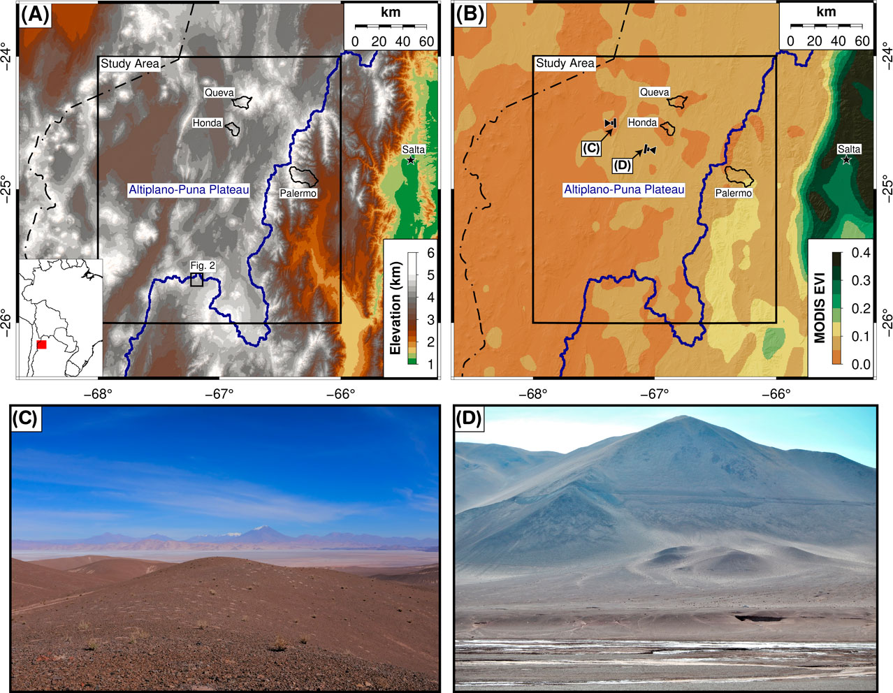
FIGURE 1. Overview of the study area in Northwest Argentina. (A) Elevation and hillshade derived from Copernicus DEM. (B) Vegetation derived from MODIS product 13C1 enhanced vegetation index 14-years average (MODIS EVI; Huete et al., 1994). No vegetation is typically defined by EVI values <0.3, and the maximum value in the study area is <0.2. Drainage boundary of the internally drained Altiplano-Puna Plateau is shown in dark blue, with catchments selected for slope and channel analysis shown in black. (C) and (D) are the photographs identified in (B), which demonstrate the smooth topography and nearly vegetation-free characteristics of the study area, with a combination of steep volcanoes, mountain ranges, flat salars, and local bedrock outcrops.

The large-scale geomorphology of the Central Andean Plateau is characterized by several internally-drained basins that formed during Pliocene and Quaternary times (e.g., Alonso et al., 1991; Strecker et al., 2007; Hain et al., 2011; Pingel et al., 2020). These have steep, fault-bounded ranges with elevations up to 6 km and basin reliefs of ∼3 km (Figure 1A). Compartmentalization of the plateau was enhanced through active volcanism and deformation (Alonso et al., 1991). During Pleistocene pluvial periods the catchments experienced increased water supply that lead to lake formation in the low-elevation parts of the basins and enhanced glacial erosion in the high-elevation parts (Bookhagen et al., 2001; Haselton et al., 2002; Luna et al., 2018). The repetitive drying of the lake beds, and the associated increase in chemical element concentration, lead to wide-spread, Lithium-rich brine formations (Godfrey et al., 2013). In addition to the steep, high-relief mountain ranges, these exceptional large (>100 km²), flat areas provide an ideal natural laboratory to study DEM variability on low slopes, akin to airplane runways at much smaller scales (Becek et al., 2016).

We assess the inter-pixel consistency over a 2° × 2° study area (∼ 220 × 220 km) shown in Figure 1, and demonstrate the geomorphic implications in three selected catchments: Honda, Queva, and Palermo, with drainage areas of 66, 94, and 219 km², respectively. The chosen catchments constitute the steeper sections of the study area, while the large flat areas (salars) provide many surfaces that should have low variability in adjacent pixels in the absence of DEM artifacts.

3 DEMs

The 1 arcsec DEMs used in the present study are shown in Table 1, with details of each dataset given below. These DEMs are derived using either photogrammetry or Synthetic Aperture Radar interferometry, each with their own issues and caveats (e.g., Nuth and Kääb, 2011; Yamazaki et al., 2017; Purinton and Bookhagen, 2017; Purinton and Bookhagen, 2018). Although additional open-access DEMs exist (e.g., MERIT, Viewfinder Panorma), these are derived from the DEMs used in the present study, and we instead focus on the un-projected products at their most recent processing release given in Table 1. We do note that the Copernicus DEM is a derived product from the TanDEM-X mission, but this is based on a significantly edited and quality controlled commercial DEM (10 m AIRBUS WorldDEM^TM; Zink et al. (2021)). The recent release and high geomorphic potential of Copernicus warrants inclusion—and recent work indicates its high quality (Guth and Geoffroy, 2021). Although these DEMs have been collected between 2000 (SRTM-NASADEM) and 2015 (TanDEM-X and Copernicus), we expect little change of the land surface during this short time period given the arid conditions and low erosion rates (Bookhagen and Strecker, 2012). Thus, despite their different dates, these datasets are comparable at the large scale of our study.

TABLE 1

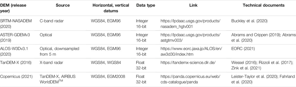
TABLE 1. Global 1 arcsec (∼30 m) DEMs compared.

The 1° × 1° tiles delivered for each DEM at 1 arcsec spatial resolution were vertically shifted to the EGM96 geoid datum (if not already in this vertical reference) with the dem_geoid function in the Ames Stereo-Pipeline (Beyer et al., 2018). The four adjacent 1° × 1° tiles were then mosaicked with gdal_merge (GDAL/OGR contributors, 2021). In a later step, the DEMs were resampled to UTM zone 19S to produce equal area (30 m) pixels using various approaches implemented in gdalwarp (GDAL/OGR contributors, 2021). We note that at 26°S the un-projected 1 arcsec pixels are 27.7 × 30.5 m (geographic longitude × latitude or Cartesian x × y) and this increases to 28.3 × 30.5 m at 24°S. This represents an ∼7–9% difference in x, y pixel length, which is removed during resampling to 30-m square UTM pixels.

3.1 SRTM-NASADEM

Collected over an 11-day mission in February 2000, the SRTM DEM—derived using C-band radar interferometry—has led to significant advances in (near) global topographic analysis (Farr et al., 2007). The ∼3 global passes of the C-band returns were used to generate DEMs at resolutions of 1 (∼30 m) and 3 (∼90 m) arcsec. Since the initial data collection in February 2000, this dataset has seen many releases and void-filling efforts (e.g., Jarvis et al., 2008), with the most recent being the reprocessed 1 arcsec SRTM-NASADEM (Crippen et al., 2016; Buckley et al., 2020). Absolute vertical uncertainties of SRTM from reference datasets on bare-earth range from ∼2–10 m depending on the chosen statistical metrics and topographic steepness (e.g., Rodríguez et al., 2006; Becek, 2008; Becek, 2014; Rexer and Hirt, 2014; Purinton and Bookhagen, 2017).

3.2 ASTER-GDEMv3

The ASTER optical sensor aboard the Terra satellite collects nadir and backwards pointing imagery at a 15 m resolution since 1999. These stereo pairs are used to generate 30 m DEMs (e.g., Kääb, 2002), which are stacked to form the ASTER-GDEM (ASTER, 2009; Tachikawa et al., 2011). The most recent ASTER-GDEMv3 was generated by stacking over 2.3 million individual DEMs (Abrams and Crippen, 2019; Abrams et al., 2020) with a varying number of stacked scenes for each row and column of the satellite orbit, with an average number of 23 (σ = 18) for the study area. Generally high absolute vertical uncertainties of the ASTER DEMs have been reported ranging from ∼6–20 m, again depending heavily on topography (e.g., Tachikawa et al., 2011; Becek, 2014; Rexer and Hirt, 2014; Baade and Schmullius, 2016; Purinton and Bookhagen, 2017).

3.3 ALOS-W3Dv3.1

The ALOS Panchromatic Remote-sensing Instrument for Stereo Mapping (PRISM), launched in 2006, provides another optical source of DEMs (Tadono et al., 2014). With along-track nadir, backward, and forward viewing cameras at 2.5 m resolution, the images are used in a similar manner to ASTER to produce tri-stereo DEMs at a resolution of 5 m, of which over 3 million were stacked to form the World 3D 5 m DEM available commercially (Takaku et al., 2014). A 1 arcsec resampled version of this dataset is available for public access, with the most recent edited and hole-filled version being the ALOS-W3Dv3.1 used in this study (EORC, 2021). Over the study area, the number of stacked PRISM DEMs used to generate the final product is on average 7 (σ = 5). Absolute vertical uncertainties for the ALOS World 3D DEMs have been reported to a more limited extent, but may be expected to range from ∼2–10 m (e.g., Purinton and Bookhagen, 2017) depending on terrain slope.

3.4 TanDEM-X

The TanDEM-X 0.4 arcsec (∼12 m) DEM is the next generation of radar-derived global topography following the SRTM. This DEM was generated by interferometric processing and stacking of >470,000 X-band radar TerraSAR-X/TanDEM-X satellite bistatic scenes collected between 2010 and 2015 (Krieger et al., 2013; Wessel, 2016; Rizzoli et al., 2017; Zink et al., 2021). These data were also resampled, without further processing via different multi-looking, to a 1 and 3 arcsec version. The bistatic scenes have also been used to create the 10 m commercial AIRBUS WorldDEM^TM (Zink et al., 2021) with careful manual editing (e.g., void filling, water-body flattening, smoothing). The 3 arcsec (∼90 m) TanDEM-X is now available for public access, but the 1 arcsec version used in the present study was received through a scientific proposal to the DLR (Zink et al., 2021). The number of individual stacked scenes in the final product is on average 7 (σ = 4) for our study area. The TanDEM-X absolute vertical uncertainty is in the range of ∼1–5 m (e.g., Purinton and Bookhagen, 2017; Wessel et al., 2018), representing a significant improvement over previous near-global DEMs.

3.5 Copernicus

The Copernicus DEM, publically released at 3 arcsec in 2019 and 1 arcsec in 2021, is a derived product from the TanDEM-X mission. This dataset is also available at 10 m resolution over Europe, and was generated from the commercial WorldDEM^TM by the European Space Agency (ESA) and AIRBUS, including additional editing and smoothing of the 1 and 3 arcsec products (Leister-Taylor et al., 2020). The recently released 1 arcsec Copernicus DEM used here should therefore represent an improvement over the similar 1 arcsec TanDEM-X (scientific product generated by the DLR from resampling the 0.4 arcsec version without editing); however, thus far, limited validation reporting exists (Fahrland et al., 2020; Guth and Geoffroy, 2021). We also emphasize that the processing and filtering steps of the commercial TanDEM-X WorldDEM^TM product leading to the Copernicus DEM are not open-source documentation. The Copernicus DEM has been assessed with ICESat-2 measurements, which indicate absolute vertical uncertainties of ∼1–3 m (Fahrland et al., 2020), and previous work to assess the WorldDEM^TM indicates similarly high accuracy of this dataset (Becek et al., 2016).

4 Motivation

Often as geomorphologists, the first assessment of DEM quality is provided by qualitative evaluation of a hillshade image with knowledge of the expected topography (Figure 2). Our study area is characterized by vegetation-free, bare-earth, and smooth surfaces, formed by diffusive transport processes in a landscape with high preservation potential (Figures 1C,D). The Copernicus DEM (Figure 2A) reproduces this expectation, while the ASTER-GDEMv3 (Figure 2B) presents a much rougher representation of the landscape, obscuring the channel, hillslope, and valley features of interest. The elevation profile in Figure 2C demonstrates the smooth versus rough qualities of these DEMs, which will have clear implications for derived metrics and flow routing on the gridded surface.

FIGURE 2

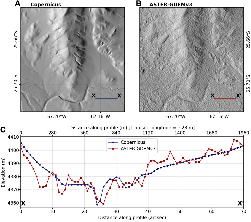
FIGURE 2. Example hillshades and elevation profiles for a ∼10-km square tile in the Central Andes (cf. Figure 1A for location). The DEMs are un-projected with 1 arcsec pixels, which translates into ∼ 28 × 30 m (longitude×latitude) pixels at this latitude. (A) Copernicus hillshade with smooth representation of topography due to high inter-pixel consistency. (B) ASTER-GDEMv3 hillshade with rough appearance due to low inter-pixel consistency. (C) ∼2000 m long elevation profiles for both DEMs from X to X’. The DEMs have not been co-registered or aligned, which can lead to offsets such as the difference in valley bottom location around 25 arcsec. Note the higher inter-pixel variability (low inter-pixel consistency) of the ASTER-GDEMv3 profile.

Our method development is motivated by a number of factors building on our previous work (Purinton and Bookhagen, 2017; Purinton and Bookhagen, 2018; Smith et al., 2019). Firstly, we wish to quantify the inter-pixel consistency (non-topographic variability, sometimes referred to as relative DEM error; e.g., Rizzoli et al. (2017)) and not point-based vertical accuracy using reference data (e.g., derived from kinematic and static dGNSS, ICESat, ICESat-2). Secondly, while an accurate control DEM (e.g., high-resolution Pleiades or SPOT7 optical DEM) could be used as a reference surface, this would require purchasing and processing these datasets, which would not cover the full geographic area of our study. Furthermore, when using reference surfaces it is necessary to align the datasets prior to comparison (Nuth and Kääb, 2011; Purinton and Bookhagen, 2018). This requires model fitting and resampling, both of which are subject to chosen parameters that can lead to additional artifacts. Thirdly, our goal is to report the impact of non-topographic variability (orbital-, sensor-, and/or processing-related artifacts) on derivatives of elevation (i.e., slope, which directly impacts other derivatives like aspect and curvature) in the context of catchment-scale geomorphic analysis of hillslopes and channels using 30 m open-access DEMs.

5 Methods

Python codes to reproduce the outlined steps, including the calculation of different metrics, are available here: https://github.com/UP-RS-ESP/DEM-Consistency-Metrics.

5.1 Consistency Metrics

Within the outlined context, we explore three options for inter-pixel consistency metrics. The different metrics can be seen in Figure 3, and details of each are provided below. All metrics are generated in small analysis windows (3 × 3 or 5 × 5 pixels, or in length ∼ 90 × 90 or ∼ 150 × 150 m), which emphasizes the variability in adjacent pixels. We view these metrics as a normalization procedure to better compare pixels to their local neighborhoods. This also can be described as a detrending or local filtering step. This is necessary, because analysis directly on the elevation pixels may mask the inter-pixel consistency signal under large-scale topographic signatures.

FIGURE 3

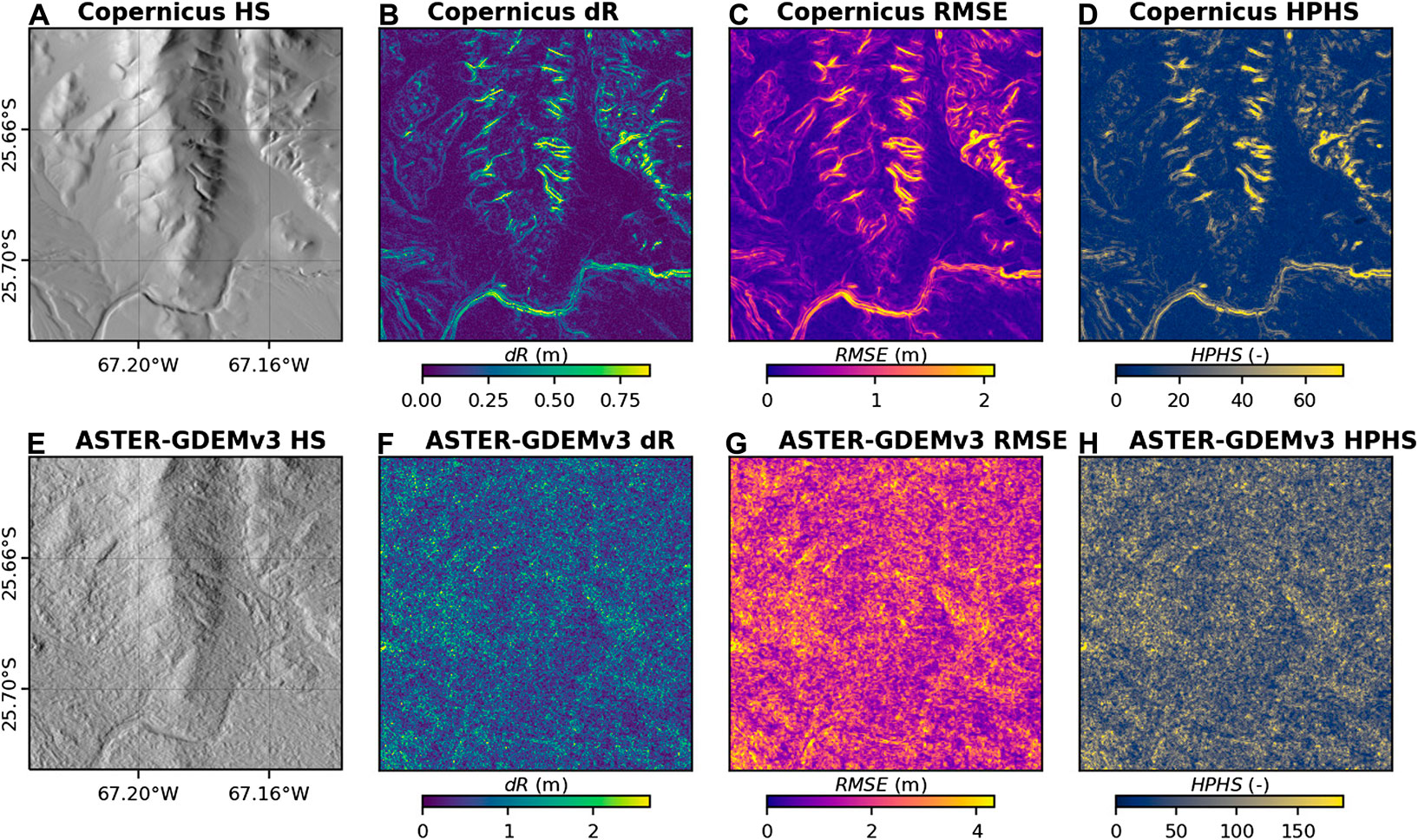
FIGURE 3. Hillshade and comparison of the three consistency metrics. ∼10-km square tiles are the same as those in Figure 2 (cf. Figure 1A for location). Top row shows (A) Copernicus hillshade with consistency metrics, (B) smoothing and differencing (dR, with units of m), (C) 3 × 3 window plane fit root mean squared error (RMSE, with units of m), and (D) hillshade azimuth rotation and maximum high-pass filter extraction (HPHS, unitless). All three metrics show a similar pattern with low values on hillslopes and planar surfaces and high values in areas of high curvature (ridges, valleys, channel banks). (E–H) Same as top row but for ASTER-GDEMv3. All colors are scaled from 0 to the 99th percentile of the value in the respective image. The rougher ASTER-GDEMv3 obscures the topographic signal, and the magnitude of all metrics is ∼2 times greater compared to Copernicus.

Because of local topographic variations, these metrics also reflect true local topographic signatures. For example, they result in high values in areas of high curvature (e.g., ridges and valleys). But at the same time, they also capture the signal of inter-pixel consistency, which has a very different spatial pattern compared to the discrete, localized ridge and valley signals of real topography. We emphasize the bare-earth and nearly vegetation-free signal of this area (Figures 1C,D): all metrics rely primarily on the assumption of field and topographic knowledge of the area of interest. If vegetation were present, we may expect a rougher surface from the spaceborne DEMs, and this will differ depending on the optical or radar collection method. Our method thus relies on some a priori knowledge of the expected surface in the study area, which can be gained through field knowledge and/or additional remote sensing data (e.g., rainfall, vegetation). But despite this, metrics can be compared between different DEMs to provide a relative assessment of inter-pixel consistency and its geomorphic implication. In the comparison step, we use the power-frequency distributions of the consistency metric to exploit the frequency, as opposed to spatial, domain. A pixel-by-pixel comparison of the various DEMs in the spatial domain would require careful sub-pixel co-registration steps (e.g., Nuth and Kääb, 2011).

5.1.1 dR: Roughness From Smoothed DEM Differencing

The first method tested was to difference the gridded elevation surface with a smoothed version of itself. We refer to this metric as roughness difference (dR, units of m), as it results in low values in areas where the DEM elevation pixels are similar (smooth) and high values in areas with rapid changes in elevation (rough). This is similar to commonly used differencing of DEMs with more accurate control DEMs, but does not rely on external data and does not require co-registration alignment between the surfaces.

With dR, the choice of DEM smoothing technique and the parameters associated with that technique are important considerations. We tested a number of convolutional smoothing methods (median, Wiener, Gaussian filters) with window sizes of 3 × 3 and 5 × 5 pixels. The different methods provided comparable results and similar spatial patterns, and the results shown in Figures 3B,F are for Gaussian smoothing with a standard deviation parameter of 0.5 in a 5 × 5 pixel window. Larger windows or standard deviations tended to over-smooth and result in excessively large dR values in areas of high curvature (ridges and valleys).

5.1.2 Root Mean Squared Error From Local Plane Fitting

In a second approach, we calculated plane fits in 3 × 3 pixel windows and assigned the resulting root mean squared error of residuals to the center pixel (RMSE, units of m). This is a local detrending of topography and similar polynomial fitting approaches are used to calculate surface roughness associated with bedrock outcrops (Milodowski et al., 2015). This is a parameter-free technique, relying on least-squares fitting and error minimization, which is less sensitive to outliers than singular value decomposition. The plane-fit RMSE results in similar spatial patterns as dR (Figures 3C,G). The drawback of this method is the computational expense of plane fitting on potentially millions of 3 × 3 pixel windows. This was optimized and multi-threaded, but still takes significantly longer to calculate than the other described metrics. Higher order fits (second or fourth degree polynomials) and different window sizes (5 × 5 pixels) were also tested, but all led to over-fitting and/or obscured the variability in adjacent pixels. We note that least-squares fitting is likely more efficient if higher-order polynomials are required for second-order derivatives (e.g., Hurst et al., 2012).

5.1.3 High-Pass Hillshade Filtering

The final metric is based directly on the derived hillshade (HS) image (8-bit integer values from 0 to 255) from the gridded elevation surface. This is calculated from slope and aspect (in radians) as:

$HS=\hspace{0.17em}\left(cos\left(\alpha \right)\times cos\left(slope\right)\right)+\left(sin\left(\alpha \right)\times sin\left(slope\right)\times cos\left(\gamma -aspect\right)\right)(1)$

where α and γ are the sun elevation and azimuth angles, respectively, in radians. Throughout our analysis, slope and aspect are calculated via the central difference method of Zevenbergen and Thorne (1987), and in the discussion we compare this with the Horn (1981) method—the two options implemented in GDAL (GDAL/OGR contributors, 2021). Different methods of calculating slope are discussed in Smith et al. (2019), where the four-neighbor Zevenbergen and Thorne (1987) method is selected based on its similarity to analytical solutions on synthetic surfaces, and its lack of smoothing.

The hillshade metric relies on the rough versus smooth appearance of the hillshade, with lower or higher values depending on the local pixel variability. Pixels with strong gradients between them have greater difference to the surrounding pixels (i.e., the inter-pixel consistency is lower). Extracting these gradients can be done with common high-pass filtering for edge detection using a 3 × 3 pixel Laplacian window (8 in the center, surrounded by −1). The magnitude of the gradient and not direction is of primary concern, so the absolute value is taken.

Since the gray-scale appearance of the hillshade also differs with sun elevation angle and azimuth, we rotated them in 10° increments from 10° to 90° for sun elevation and 45° increments from 0° to 315° for azimuth. Following this, the maximum value at each pixel was taken from the stack of high-pass filtered hillshades, producing our unitless HPHS metric. We found that changing the sun angle only changed the magnitude and not the relative spatial pattern of HPHS, so we applied a consistent 25° sun angle. Further, only taking the four cardinal directions (0°, 90°, 180°, 270°) were sufficient to extract the spatial pattern.

5.1.4 Selection of Inter-Pixel Consistency Metric

HPHS is a fast calculation because slope and aspect need only be calculated once for every pixel and then the four hillshades (four azimuths) and their gradients can be derived quickly. As all three metrics showed similar spatial patterns, we chose to continue with HPHS. Although the physical units (m) associated with the other methods provide meaningful magnitude, the dR metric requires selection of a smoothing method and smoothing parameters, while fitting planes across the grid to extract RMSE is computationally expensive. Furthermore, unlike the other two options, the HPHS metric includes slope and aspect information, and is closely linked to qualitative DEM assessment of hillshade images, which remains an important and useful visual check on quality (Polidori and El Hage, 2020).

5.2 HPHS Fourier Frequency Analysis

Having selected an inter-pixel consistency quality metric that accentuates the variability in adjacent pixels, we seek to quantify it. For this, we turn to frequency analysis using the two-dimensional discrete Fourier transform (2D DFT) on the HPHS grids. This converts gridded values from the spatial to the frequency domain, which provides information about the amplitude and periodicity of the grid. In other words, the 2D DFT quantifies the variance at discrete wavelengths (units of distance, where frequency = wavelength⁻¹). This technique has been used in prior assessments of DEM quality and artifact removal (Arrell et al., 2008; Purinton and Bookhagen, 2017; Yamazaki et al., 2017), and this and other wavelet-based frequency analysis are increasingly popular for characteristic landscape scaling and feature identification (e.g., Perron et al., 2008; Booth et al., 2009; Roering et al., 2010; Hooshyar et al., 2021; Struble et al., 2021; Wapenhans et al., 2021).

5.2.1 2D DFT Calculation

We follow the methods outlined in Perron et al. (2008) and Purinton and Bookhagen (2017) to take the 2D DFT of a square matrix of HPHS values, h (x, y), with N_x × N_y measurements spaced evenly by Δ_x and Δ_y:

$H\left(k_x,k_y\right)=\sum _{m=0}^{N_x-1}\sum _{n=0}^{N_y-1}h\left(m{\mathrm{\Delta }}_x,n{\mathrm{\Delta }}_y\right)e^{-2\pi i\left(\frac{k_{x}m}{N_x}+\frac{k_{y}n}{N_y}\right)}(2)$

where k_x and k_y are wave numbers and m and n are indices of h. Further pre-processing details (e.g., detrending and windowing to reduce spectral leakage) can be found in Perron et al. (2008), and are also documented in the provided Python codes: https://github.com/UP-RS-ESP/DEM-Consistency-Metrics. The 2D DFT outputs an array with the amplitudes of the frequency components in x and y, given as:

$f_x=\frac{k_x}{N_x{\mathrm{\Delta }}_x},f_y=\frac{k_y}{N_y{\mathrm{\Delta }}_y}(3)$

The spacing, Δ_x and Δ_y, can vary with orientation for gridded values, and the lowest wavelength (highest frequency, a.k.a. the Nyquist frequency) that can be resolved is 2Δ_x,y. For a 1 arcsec grid this translates into a minimum wavelength of 2 arcsec, and for a 30 m resampled grid into 60 m. The wavelength of a given H (k_x, k_y) grid element is given as:

$\lambda =\frac{1}{\sqrt{f_x^2+f_y^2}}(4)$

The quantity $\sqrt{f_x^2+f_y^2}$ is the radial frequency and assigns every element in (k_x, k_y) to a specific frequency. Given this relationship, the minimum wavelength returned by the 2D DFT on a square grid is actually above the Nyquist frequency, to account for the power at adjacent (x-, y-, or diagonal) pixels. We emphasize that these are not periodic features resolvable by the 2D DFT, since they are only single pixel (not multi-pixel) steps. For a 1-arcsec grid the maximum x and y frequencies (Nyquist frequency) are f_x = f_y = 1/2 arcsec⁻¹, and thus the minimum wavelength returned is λ = 1.4 arcsec, and for a 30 m grid the minimum wavelength is λ = 42 m.

From the 2D DFT, the power spectrum can be approximated using the DFT periodogram:

$P_{DFT}\left(k_x,k_y\right)=\frac{1}{{N_x}^2{N_y}^2}|H\left(k_x,k_y\right){|}^2(5)$

The P_DFT array is a measure of the variance of h and has units of amplitude squared, which in our case is unitless when h is HPHS. The spectral power is a measure of the mean-squared amplitude at a given frequency or frequency range. From this power spectrum we can quantify both low-frequency (long-wavelength) periodic features at frequencies lower than the Nyquist frequency (≥2-arcsec or ≥60-m wavelengths) and high-frequency (short-wavelength) variance at frequencies higher than the Nyquist frequency (1.4- to < 2-arcsec or 42- to <60-m wavelengths).

5.2.2 Long-Wavelength Peaks

In the first step of Fourier frequency analysis, we quantify periodic artifacts in the DEMs with wavelengths above the Nyquist limit utilizing the 1 arcsec DEMs. Here we use the un-projected grids, since resampling the DEMs to 30-m square UTM pixels will introduce additional periodic artifacts. We compare resampling schemes in a separate step.

Following Purinton and Bookhagen (2017), the 2D power spectrum is first plotted in one dimension (1D) as radial frequency versus mean-squared amplitude. A linear regression (a power-law fit in log-log space) through 20 logarithmically spaced wavelength bins (at their median amplitude) is then calculated and used as the background spectrum. Both the 1D and 2D power spectra can be normalized by dividing the original by this background spectrum using the power-law fit coefficients applied to the 1D and 2D frequencies (Perron et al., 2008). This results in the normalized power, which provides the opportunity to observe longer-wavelength variability associated with orbital-, sensor-, and/or processing-related artifacts. The signature of these long-wavelength (≥2 pixel) features are anomalously large power values (peaks) in the normalized spectrum.

These peaks can also be associated with topographic variability from ridge and valley spacing (Perron et al., 2008), and larger scale topographic trends of mountain ranges and salt flats, but we expect such quasi-periodic features to have more diffuse power signatures as opposed to repetitive patterns from DEM artifacts (Arrell et al., 2008; Purinton and Bookhagen, 2017). As these artifacts are low in variance compared to the variance of adjacent pixels, they require large areas of analysis to become apparent. Thus, we tiled each DEM into non-overlapping ∼60-km square tiles (resulting in 16 tiles) and calculated the HPHS and normalized power spectrum for each tile.

To objectively determine the presence of these peaks and their wavelength, we rely on the ratio of the binned maximum envelope of normalized power in a given DEM tile to the same power envelope in the Copernicus DEM tile. This assumption is based on the high inter-pixel consistency suggested by the Copernicus DEM hillshade (Figure 2) and three metrics (Figure 3), as well as the high-quality WorldDEM^TM source. Point-based validation using ICESat also indicates a relatively high vertical accuracy of 2.17 m at the 90th percentile (LE90; Fahrland et al., 2020). Therefore, the Copernicus normalized power spectrum in a given tile should represent the background power associated primarily with topographic variability.

With this assumption, we use 41 different logarithmically spaced bins of wavelength from 50 to 250 in steps of 5 bins to calculate a maximum normalized power envelope (the maximum value in each bin). We restrict the bin range to ≥2-arcsec wavelengths (2 pixels, ∼60 m) to 165-arcsec wavelengths (165 pixels, ∼5,000 m), as initial testing showed no spectral peaks at longer wavelengths in the HPHS grids.

We then take the ratio of the maximum envelope to the same envelope (same tile, same bins) from the Copernicus DEM and select peaks that are three times greater than the standard deviation of this ratio (DEM of interest : Copernicus). We remove any identified peaks with ratio values <2 (below twice the Copernicus maximum). With the peaks selected and their bin value (wavelength) recorded, we can apply a mask to the 2D DFT at the discrete peak wavelength ±5%. The range was selected to allow some variability in the exact peak location given the range of bins and shifting peak location. We then search this wavelength range in the 2D DFT for the maximum value. Since the 2D DFT contains information on the orientation of the peak (θ):

$tan\left(\theta \right)=\frac{k_y{\mathrm{\Delta }}_y}{k_x{\mathrm{\Delta }}_x}(6)$

we can also retrieve the direction of the periodic sinusoidal wave at the peak value.

With 16 tiles and 41 bins the peak finding is carried out 656 times per DEM (SRTM-NASADEM, ASTER-GDEMv3, ALOS-W3Dv3.1, TanDEM-X), leading to potentially thousands of peak identifications. Varying the logarithmic binning during peak selection acts to approximate uncertainties on the peak wavelength and orientation. The nature of the binning may dilute the exact wavelength and orientation, so the results are assessed with 2D histograms of peak wavelength and orientation, where each histogram bin contains the number of peaks found.

5.2.3 High-Frequency Variance

The long-wavelength peaks are useful to identify and quantify DEM artifacts, but we are primarily interested in the consistency of adjacent pixels that will impact slope, aspect, curvature, and flow-routing based on neighborhood calculations (typically 3 × 3 pixel window). As stated, the shortest wavelength periodic feature resolvable by the 2D DFT is twice the pixel size. However, as the sum of the P_DFT over all frequency bins (i.e., the integral) approximates the variance of the input grid (e.g., HPHS), we can draw a direct connection between the percent of non-normalized power at a given wavelength range and variability of these pixel steps. Thus, in this second Fourier analysis step, we do not quantify periodic signals, but rather the proportion of total variance in the HPHS grid that is accounted for by adjacent pixel steps.

In this case, we do not need to be concerned with longer-wavelength artifacts introduced by resampling the grids to square pixels, though we do note that the long-wavelength peak finding analysis can also be used to quantify resampling artifacts. Furthermore, resampling is typically the first step in topographic analysis with DEMs and is done prior to any slope or flow-routing calculations. Thus, prior to the high-frequency analysis, we resample all grids to 30-m square pixels in UTM zone 19S using the nearest neighbor, bilinear, cubic, cubic spline, lanczos, and average resampling schemes in gdalwarp (GDAL/OGR contributors, 2021). This also provides the opportunity to assess differences in inter-pixel consistency resulting from different resampling schemes.

Following resampling from 1 arcsec to 30 m DEMs, we take the percent of total power (non-normalized) at the 42- to <60-m wavelengths (adjacent pixels) and compare this between all five DEMs. As we are not interested in peak identification and only local variance signals, we used a smaller size of ∼20-km square tiles (resulting in 96 tiles) for each DEM, from which we calculated the HPHS, 2D DFT, and percent of power (variance) above the Nyquist frequency. The 96-value distributions for each DEM and each resampling scheme are visualized using boxplots.

5.3 Geomorphic Implications

With the longer-wavelength peaks and higher-frequency variance quantified, we seek to compare their effects on geomorphic analysis. Calculations are always done on the UTM projected grids (30 m resolution, resampled via cubic spline).

In a first step, we calculate the slope distribution for each of the three test catchments (Figure 1). We focus only on slope as it is the first derivative of elevation, and inaccuracies caused by low inter-pixel consistency in this metric will manifest in other DEM derivatives, such as curvature and aspect. Gridded slope in degrees is calculated in a 3 × 3 pixel window following the standard Zevenbergen and Thorne (1987) algorithm. The slope distributions for each DEM in each catchment are then compared and connected to the inter-pixel consistency quantified with the Fourier analysis.

We also extract flow networks for each catchment via the D8 algorithm (O’Callaghan and Mark, 1984) using each DEM and compare the longitudinal river profile of the longest channel (trunk stream). We assess the difference in normalized channel steepness (k_sn):

$k_{sn}=S{A}^{-{\theta }_{ref}}(7)$

where S is channel gradient, A is drainage area, and θ_ref is a reference channel concavity. This is a standard analysis in tectonic geomorphology used to identify channel knickpoints and their tectonic and climatic forcings (e.g., Wobus et al., 2006). Drainage extraction and k_sn calculations (using a θ_ref = 0.45 and minimum drainage area threshold of 0.1 km²) were done with LSDTopoTools (Mudd et al., 2019), which implements the integral approach to channel steepness (Perron and Royden, 2013), with the addition of segmented fitting (Mudd et al., 2014).

In a final step, we explore the effect of inter-pixel consistency on local channel gradient calculations (channel node to channel node along the profile). We follow the method of Clubb et al. (2019), and apply linear regressions to local windows of connected channel nodes to extract slope. We vary the window size of gradient calculation over 3, 5, 7, 9, and 11 nodes (∼90–330 m channel segments) to explore its effect on reducing artifact-related variance in the gradient.

6 Results

Here, we focus on the detailed steps and results for Fourier analysis of HPHS. We choose to present the results of the geomorphic analysis in the discussion section, as they are pertinent to discussions of inter-pixel consistency, and to the suggestions and caveats of DEM selection.

6.1 Long-Wavelength Peaks

6.1.1 Normalized Power

An example power spectrum for the HPHS metric calculated on one ∼60-km SRTM-NASADEM tile at 1 arcsec resolution is shown in Figure 4. This includes the normalized power (Figure 4C), which was calculated via the 1D power-law fitting and normalization on the same tile (Figure 5). Roughly north-south trending mountain ranges, with flat salars and valleys between, are apparent in the hillshade image in Figure 4A. The HPHS calculated on this hillshade (Figure 4B) shows highest values on the ridges and valleys (topographic signature), but also some high values on low-slope areas. Furthermore, there is a clear striping pattern apparent in this image, which is the SRTM artifact associated with mast-oscillation during collection (Farr et al., 2007; Crippen et al., 2016). The normalized power from the HPHS (Figure 4C) has strong peaks associated with this pattern that are indicated as P1–4. These peaks do not always occur at consistent orientations, but they do have distinct and consistent wavelengths. On the other hand, as expected, the quasi-periodic north-south trending topography manifests as a diffuse and low-power long wavelength cluster with an approximately east-west orientation. We also note that high power values are clustered in the corners of the power spectrum, which hold the 1.4- to < 2-arcsec wavelengths.

FIGURE 4

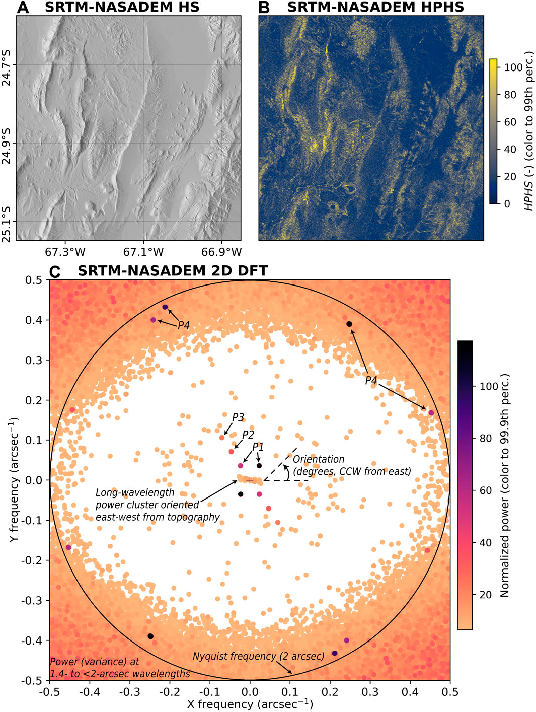
FIGURE 4. Example of a 2D DFT analysis of HPHS in a ∼60-km square tile for an un-projected 1 arcsec DEM. (A) SRTM-NASADEM hillshade. (B)HPHS calculated on the tile, with color scaled from 0 to the 99th percentile. Note the distinct NW-SE striping pattern, particularly in the northwest. (C) 2D DFT periodogram, showing the normalized amplitude (power) in frequency space. The lowest frequencies (longest wavelengths) are in the center of the plot, and wavelength (frequency) decreases (increases) away from the center. Any two adjacent quadrants in the plot contain all the information, which is reflected through the central origin. The associated 1D DFT is shown in Figure 5. For visualization purposes, the periodogram was morphologically dilated to increase the size of the discrete, high-power peaks and values below the 50th percentile were excluded (colored white). Note the peaks (P1–4) orientated at ∼120° (counter clockwise (CCW) from east), with P4 (∼60 m wavelength) occurring at other orientations. The signal of north-south orientated topography can be seen in the diffuse east-west power cluster at the lowest frequencies, and the high power (high variance) above the Nyquist frequency (black circle) is shown by the high values in the corners.

FIGURE 5

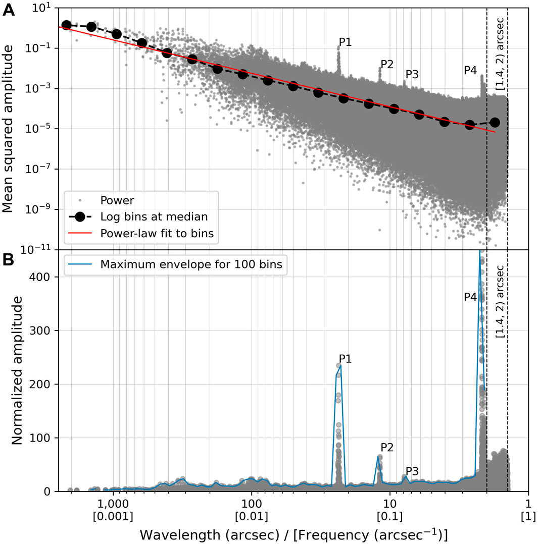
FIGURE 5. Example of a 1D DFT normalization procedure for the same 1 arcsec ∼60-km square SRTM-NASADEM tile shown in Figure 4A Mean-squared amplitude (a measure of spectral power provided by the P_DFT in Eq. 5) of HPHS (unitless) with log-spaced frequency bins and power-law fit to the bin medians. (B) Amplitude (power) normalized by the power-law fit, with a maximum envelope connected in 100 log-spaced frequency bins ≥2-arcsec wavelengths. The high-frequency power (adjacent pixels) returned by the radial frequency (cf. Eq. 4) are indicated by the dashed vertical lines from 1.4- to < 2-arcsec wavelengths. The peaks (P1–4) shown in Figure 4C are indicated.

Figure 5A shows the radial 1D power spectrum from the P_DFT. The amplitude decreases with increasing frequency, leading to an approximate power-law distribution in the binned data. The labelled peaks (P1–4) are particularly prominent in the normalized power spectrum (Figure 5B). These are clearly anomalous signals related to DEM artifacts and not topographic signatures, which have much broader peaks (Perron et al., 2008; Purinton and Bookhagen, 2017).

6.1.2 Peak Finding

The peaks identified in Figures 4C, 5B are objectively extracted using the described peak finding method. In order to address uncertainties associated with the logarithmic binning of the data, we have performed the binning with different step sizes and present here the averaged result.

Figure 6 presents two iterations (of 41 bin numbers) for 75 and 250 bins in the same 1 arcsec SRTM-NASADEM tile used in Figures 4, 5. The normalized HPHS power spectrum for the same tile is calculated for the 1 arcsec Copernicus DEM and the ratio of maximum envelope of the SRTM-NASADEM: Copernicus is taken, from which peaks are identified (3 × standard deviation and >2). Notably, not all expected peaks (P1–4) are found, and the peaks differ slightly between each bin step.

FIGURE 6

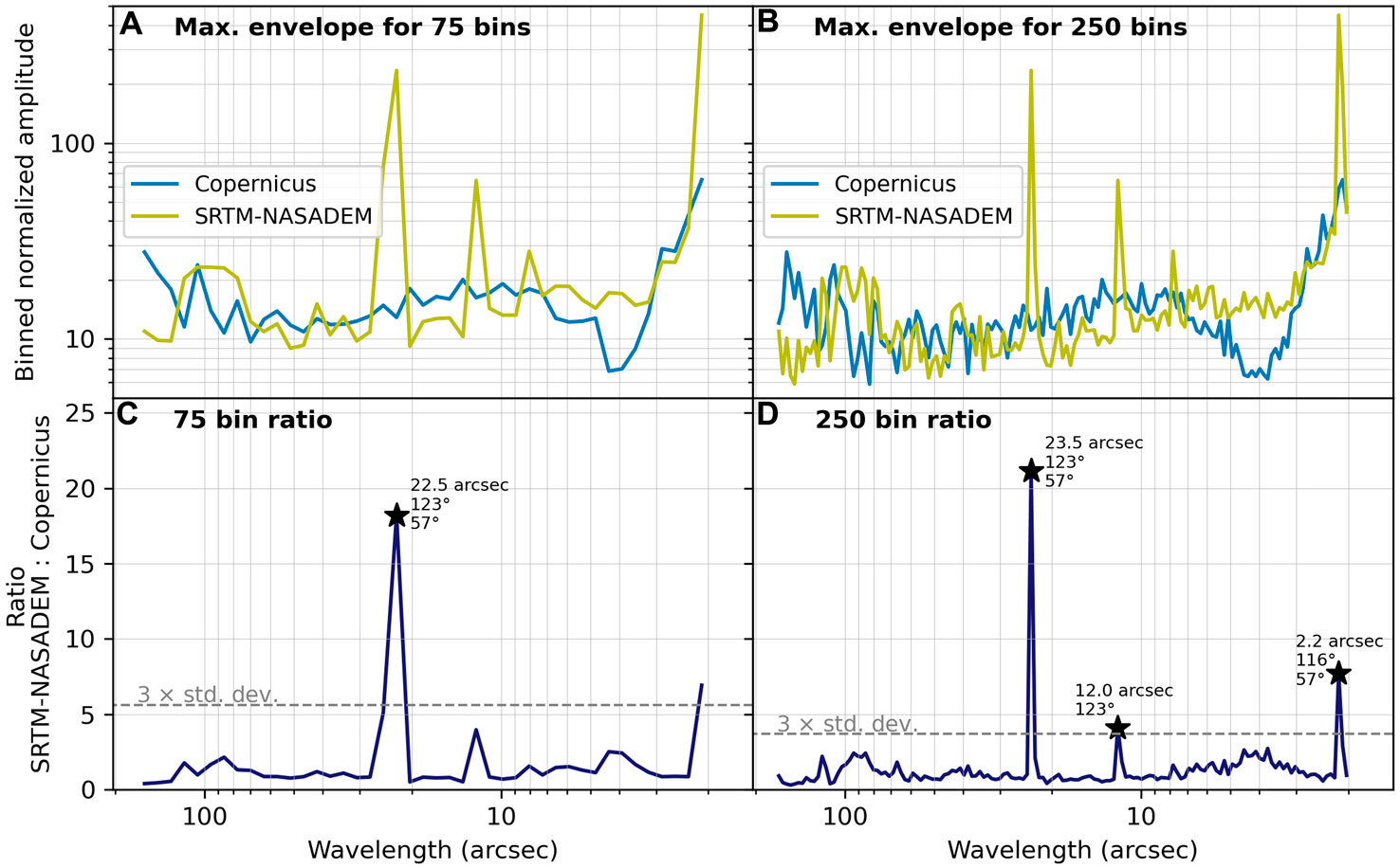
FIGURE 6. Example 1D DFT peak finding procedure for the same 1 arcsec ∼60-km square SRTM-NASADEM tile shown in Figures 4, 5. The result for 75 bins is shown in (A) and (C), and for 250 bins in (B) and (D). The maximum HPHS power envelope from the same tile for Copernicus is used for normalization to highlight the anomalous peaks. The minimum and maximum wavelength for binning and peak identification is set to 2 and 165 arcsec (∼60–5,000 m), respectively. Peaks are automatically selected in the ratio plot if they are 3× the standard deviation and above a value of 2. The wavelength of the peak is identified, and the orientation of the maximum wavelength in degrees counter clockwise from east are found by searching for the maximum value in the associated 2D DFT plot at this wavelength ±5%. Peaks are labelled with their wavelengths and orientations. Not all peaks are found, but the procedure is repeated for 41 bin numbers (50–250 in steps of 5) for fitting uncertainty estimation.

The process of peak finding is repeated 656 times (41 bin steps × 16 tiles) for each DEM (SRTM-NASADEM, ASTER-GDEMv3, ALOS-W3Dv3.1, and TanDEM-X), always using the Copernicus DEM as the control (denominator in the maximum envelope ratio). This generates an ensemble of peak wavelengths (identified in 1D) and orientations (identified in 2D given the wavelength). Thus, despite each tile and bin step potentially missing some peaks and slightly shifting their wavelengths, we can visualize the results with 2D histograms of wavelength and orientation in Figure 7. The TanDEM-X DEM is not included as no peaks >2 in its ratio against the Copernicus DEM were found. Although our peak finding covered a wavelength range of 2–165 arcsec, no peaks >25 arcsec (∼750 m) were found.

FIGURE 7

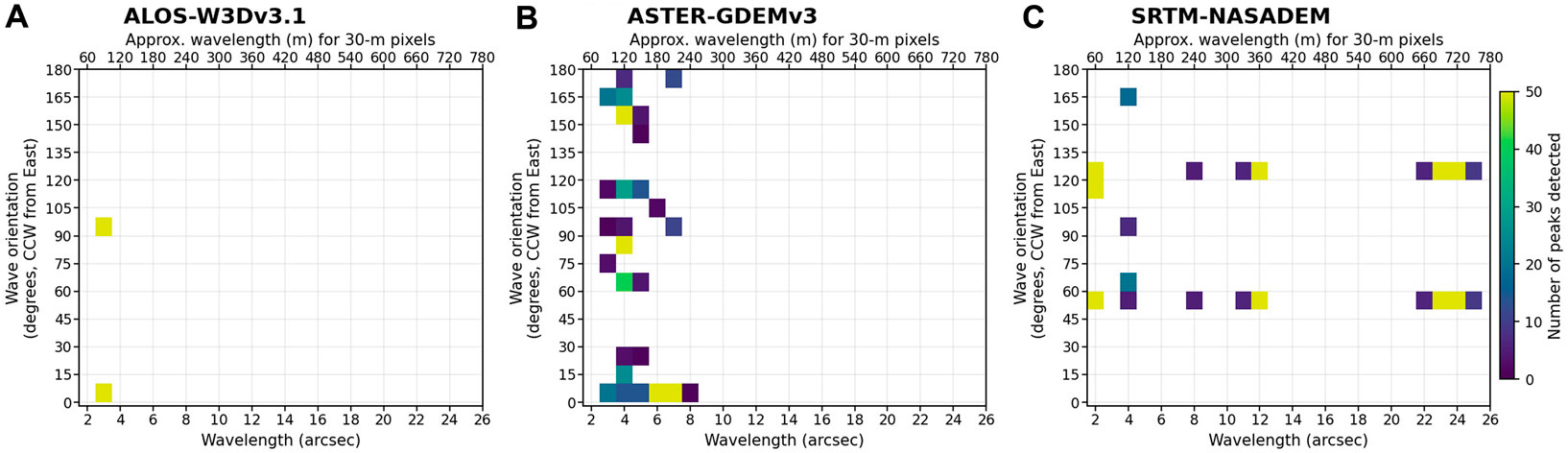
FIGURE 7. HPHS power peaks found for all 16 square (∼60-km) tiles. Peak finding is done on un-projected 1 arcsec DEMs, and the upper x-axis label shows the approximate wavelength in meters at 30-m pixel resolution. A 2D histogram is used to show the number of peaks, since many peaks are identified in the 41 separately binned ratio plots for each of the 16 tiles (656 iterations). The histogram has bins in 1-arcsec wavelength steps (1 pixel) and 10° orientation steps. The resulting peak count at each wavelength and orientation bin is shown for (A) ALOS-W3Dv3.1, (B) ASTER-GDEMv3, and (C) SRTM-NASADEM. No peaks were found above 25 arcsec (25 pixels, ∼750 m), nor for the TanDEM-X. The colorscale is limited to 50 peaks, but often more were found. Orientation is given as counter clockwise (CCW) from east, thus 0° is east, 45° is northeast, 90° is north, and so on.

In Figure 7A, the ALOS-W3Dv3.1 has concentrated peaks at 3 arcsec (∼90 m) with orthogonal east-west and north-south orientations. On the other hand, the ASTER-GDEMv3 (Figure 7B) has a range of peak wavelengths from 3–7 arcsec (∼90–210 m) with less consistent orientation. We note that bins with a low peak count are possible artifacts of the peak-identification method. With this in mind, we suggest that the ASTER-GDEMv3 peaks are particularly concentrated at 4 arcsec (∼120 m) and 6–7 arcsec (∼180–210 m), and possibly in an approximately north-south and east-west orientation, though this is highly variable. The SRTM-NASADEM presents particularly notable results (Figure 7C). The peaks occur at consistent wavelengths (>50 peaks found) of 2 arcsec (∼60 m), 12 arcsec (∼360 m), and 23–24 arcsec (∼690–720 m). Furthermore, their orientations are consistently ∼60° and ∼120° counter clockwise from east, which corresponds to a north-northeast and north-northwest repetitive sinusoidal pattern.

6.2 High-Frequency Variance

The peaks quantified in Figure 7 correspond only to the ≥2-arcsec (2-pixel) wavelengths in the HPHS grid on the un-projected 1 arcsec DEMs. The sinusoidal DEM artifacts at longer wavelengths (Figure 7) are notable, but the shorter-wavelength variance has the primary impact on inter-pixel consistency in local windows used for many topographic calculations. The variance (percent of total power) corresponding to the 42- to <60-m wavelengths (i.e., adjacent x, y, and diagonal pixels) for the 30-m UTM resampled DEMs is quantified in 96 square (∼20-km) tiles in Figure 8. Here, we are able to use a smaller tile size to extract a larger distribution (more tiles compared to 60-km tiling), since we are not interested in the longer-wavelength periodic features, which are more subtle (lower total percent of power) and only become prominent when considering larger areas in the frequency analysis.

FIGURE 8

FIGURE 8. Percent of total HPHS power (variance) at 42- to <60-m wavelengths. Here, the DEMs are first projected in UTM zone 19S and resampled to 30-m square pixels. Three resampling schemes are shown, with additional results in Supplementary Figure S2. For each DEM, the high-frequency power was calculated for 96 square (∼20-km) tiles. The distributions are shown as boxplots with center line showing the median, box showing the interquartile range (IQR), and caps showing values at ± 1.5×IQR. Outliers are not shown. For all DEMs, except the SRTM-NASADEM, the nearest neighbor resampling has the highest variance and these decrease with larger window sizes (bilinear) and higher order (cubic spline) approaches. The relative impact of smoothing is strongest for the ASTER-GDEMv3. We note that larger-window resampling schemes also affect real topographic features.

Figure 8 only presents the results for the nearest neighbor, bilinear, and cubic spline resampling schemes, while Supplementary Figure S2 shows the average, cubic, and lanczos resampling methods. The percent of power at 42- to <60-m wavelengths can be interpreted as the relative inter-pixel consistency between the five DEMs. Lower values (median and interquartile range <7.5%) for the Copernicus and TanDEM-X correspond to relatively higher inter-pixel consistency (smoother appearance in Figure 2A), compared to the lower inter-pixel consistency implied by the higher percent of power values (median and interquartile range >7.5%, often >10%) for ALOS-W3Dv3.1, ASTER-GDEMv3, and SRTM-NASADEM. We note that the TanDEM-X has somewhat higher percent of power at < 60-m wavelengths compared to the Copernicus DEM (derived from the same source data as the TanDEM-X research product), which is a result of the careful editing and smoothing of the Copernicus DEM. This is difficult to discern from the plot, but, for example, the 25th percentile of the Copernicus boxplot for the cubic spline resampling is at ∼2.49%, and at ∼2.51% for the TanDEM-X. In most cases, variance is decreased (inter-pixel consistency is increased) going from nearest neighbor to bilinear to cubic spline resampling, with the SRTM-NASADEM being the exception. The variance is also decreased going from lanczos to cubic to average resampling in Supplementary Figure S2, but the cubic spline resampling in Figure 8 produces the greatest reduction in adjacent pixel variance.

7 Discussion

The Fourier analysis allows us to quantify inter-pixel consistency between the five (near) global 1 arcsec DEMs. Pre-processing the gridded elevations, via local detrending with our HPHS metric, highlights the signals associated with inter-pixel consistency. In the following, we first discuss caveats of the method. We then connect the observed long-wavelength and high-frequency patterns with possible causes and with DEM sources. Finally, we explore the geomorphic impacts of the Fourier-quantified inter-pixel consistency and make suggestions for DEM selection.

7.1 Considerations and Caveats of Inter-Pixel Consistency Fourier Analysis

As previously stated, the use of an inter-pixel consistency metric for comparing DEMs relies on some assumptions. First and foremost, the characteristics of the study area must be known via field and topographic knowledge or observation in satellite imagery or other remotely sensed datasets (e.g., vegetation, rainfall). The presence of vegetation or snow and ice would modify the performance of a given DEM. For instance, depending on the radar wavelength (e.g., C-band for SRTM and X-band for TanDEM-X), there will be different penetration depths of canopy (e.g., Carabajal and Harding, 2006; Hofton et al., 2006; Wessel et al., 2018) and snow (e.g., Rignot et al., 2001; Rossi et al., 2016), and for optical DEMs (e.g., ASTER and ALOS) only the top surface is recorded. Our study area presents an opportunity to examine inter-pixel consistency under ideal conditions: arid, nearly vegetation-free, and mixed steep (mountain ranges) and flat (salars) topography (Figures 1C,D). Field observations and field measurements of our study area show very low inter-pixel variations at 30 m spacing, and we can interpret deviations in the consistency metrics to be DEM artifacts and not topographic signal. We expect that the observed artifacts will be present in other regions, and these will be further impacted by land-surface characteristics, which may mask or amplify the artifacts in complex ways.

A second assumption was used for objective peak identification. Here, we assumed that the Copernicus DEM was free of longer-wavelength artifacts and used this to take a normalizing ratio to highlight anomalous peaks in spectral power in the other datasets. This step is justified by the high-quality source of the carefully edited AIRBUS WorldDEM^TM—based on the original TanDEM-X data. This said, the ratio step is only necessary for automatic peak identification. In many cases, the wavelength peaks could be graphically identified given their prominence against background values (high power, e.g., Figure 5), and the method is useful as a stand-alone (without reference data or another DEM) approach for the identification of ≥2-pixel wavelength artifacts. In a conservative sense, the automatic identification of repetitive signals on the DFT spectrum presented in this study is only relative to the Copernicus DEM. However, the second step to quantify the variability of high-frequency (<2 pixel) adjacent pixels in UTM 30-m reprojected DEMs does not rely on a reference surface, and instead acts as a comparative metric between DEMs, under the first assumption of field characteristics: are smoother or rougher local topographic surfaces expected? This also provides quantitative assessment of differences in resampling, which is a key first step in topographic analysis.

We note that the DFT can only be carried out on void-free tiles, and all DEMs used here are void-filled versions. This is accomplished by a combination of interpolation (e.g., Copernicus voids ≤16 pixels in size interpolated from surrounding terrain; Leister-Taylor et al., 2020) and/or replacement with other newer or older DEMs (e.g., SRTM-NASADEM voids filled by ASTER-GDEM and ALOS-W3D; Buckley et al., 2020). We do not expect the void-filling to alter the consistency metrics reported here, as these are discrete areas making up a small portion of the DEMs, particularly in our arid study area, where atmospheric and land-cover challenges to spaceborne DEM collection and processing are minimized.

Fourier analysis performed directly on elevation grids are taken to characterize landscape scales (Perron et al., 2008; Hooshyar et al., 2021), identify and quantify pit-and-mound (Roering et al., 2010) or landslide (Booth et al., 2009) topography, and even identify and remove striping artifacts in lidar (Arrell et al., 2008) and SRTM DEMs (Yamazaki et al., 2017; Purinton and Bookhagen, 2018). Akin to these studies, we previously calculated the 2D DFT directly on the gridded elevation values to highlight artifacts in 2–8 pixel wavelengths for an 8 × 14-km clip of the ALOS-W3D 5 m commercial DEM in Purinton and Bookhagen (2017). This may be appropriate for higher-resolution DEMs (<10 m) in small study areas, but the large-scale (60-km tiles) and diversity of topography in the 1 arcsec DEMs used here necessitates a neighborhood filtering approach.

In Figure 9, we present a normalized 2D power spectrum calculated directly on the elevation values for the same SRTM-NASADEM tile shown in Figure 4. The influence of longer (i.e., several dozen to hundred pixel steps) topographic wavelengths of valleys, ridges, mountain chains, and salt flats reduces and/or obscures the inter-pixel consistency, and the periodic signals of artifacts. By locally detrending the topography using a metric like HPHS, the wavelengths of nearby pixel variability are highlighted, preparing the DEM data for a more meaningful inter-pixel consistency analysis. Furthermore, this and other metrics (internal smoothing dR, plane-fit RMSE), provide an additional visual assessment of DEM quality and the spatial patterns of noise, closely tied to hillshade observations (Figure 2).

FIGURE 9

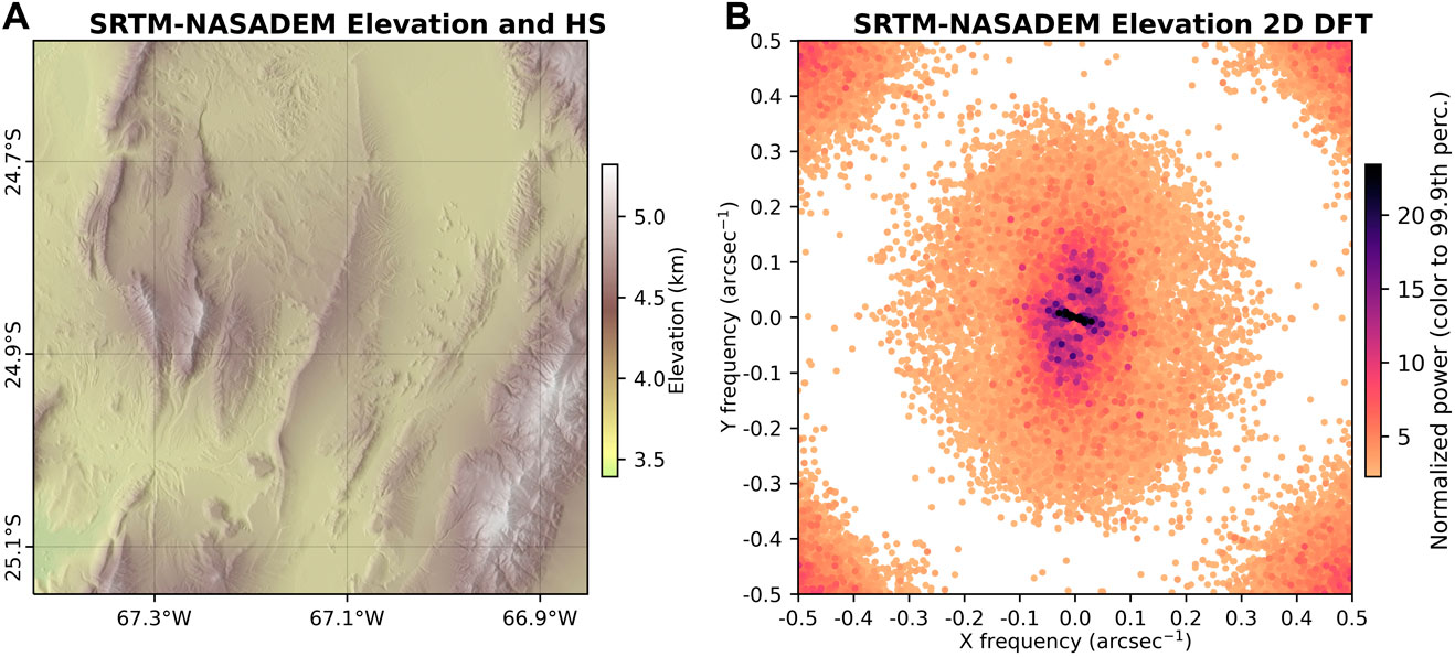
FIGURE 9. 2D DFT analysis of elevation in the same 1 arcsec ∼60-km square tile as Figure 4. (A) SRTM-NASADEM hillshade and elevation. (B) 2D DFT periodogram, showing the normalized amplitude (power) in frequency space. As in Figure 4, for visualization purposes the 2D DFT was morphologically dilated to increase the size of the discrete, high power peaks and values below the 50th percentile were excluded (colored white). Without a local detrending procedure to accentuate inter-pixel consistency (e.g., HPHS) topographic signals become more prominent, and the artifact peaks and high-frequency variance are reduced and/or obscured. In this example, the approximately north-south trending ridges create the highest power signals in (B).

In another step, we tested the result of increasing the kernel size for high-pass filtering in the HPHS calculation (Supplementary Figure S1). Our 3×3-pixel filter particularly accentuates the variability of adjacent pixels—and notably also accentuates longer-wavelength periodic patterns—whereas increasing the high-pass kernel size to 5 × 5 pixels demonstrates that while the longer-wavelength patterns are still visible in the 2D DFT, the high-frequency pixel-to-pixel variance is reduced (Supplementary Figure S1).

A recent review by Polidori and El Hage (2020) highlights the need for different approaches of inter-pixel consistency reporting to improve understanding of DEM quality beyond vertical accuracy. This is key given increases in quantitative geomorphometry and dissemination of DEMs from many (sometimes poorly understood) sources (Sofia, 2020). The metrics developed here provide a more suitable assessment of DEM quality compared to point-based vertical accuracy, which does not account for the spatial variability of DEM vertical errors that impact derivatives of elevation. These metrics do not use reference surfaces (e.g., Kramm and Hoffmeister, 2019) to assess spatially continuous patterns of vertical error, which requires co-registration of the surfaces. Co-registration of the DEMs would be particularly important for the case of the ALOS-W3Dv3.1, which has the pixel edges aligned to integer coordinates in latitude and longitude (EORC, 2021), rather than the pixel centers as in all other DEMs, leading to a half pixel offset. Our Fourier steps transform the analysis from the spatial to the frequency domain, thus negating this co-registration requirement (Nuth and Kääb, 2011), which may introduce additional uncertainties from model fitting and/or resampling.

7.2 Causes of Inter-Pixel Consistency Observations

The Copernicus and TanDEM-X DEMs have the highest inter-pixel consistency (Figure 8), with a generally smooth representation of the arid landscape in our study area. The TanDEM-X DEM is a research-grade product and still contains some noise over water bodies and on steep slopes (particularly eastern and western facing slopes facing the TerraSAR-X/TanDEM-X satellite look direction). This manifests in slightly higher <60-m wavelength variance for the 30-m projected tiles, but the TanDEM-X does not have any longer-wavelength (>2 arcsec) anomalies in the 1 arcsec tiles.

The long-wavelength artifacts in the SRTM-NASADEM have previously been identified by many authors (e.g., Gallant and Read, 2009; Yamazaki et al., 2017; Purinton and Bookhagen, 2018; Grohmann, 2018). Here, we build on this previous work and develop another approach to quantify the wavelengths and orientations of these artifacts. The mast-oscillations during collection are responsible for the original artifacts (Farr et al., 2007), and this is clear from the north-northeast and north-northwest orientation of the waves along the ascending and descending passes of the shuttle mission. However, the multiple wavelengths (2, 12, and 23–24 arcsec; Figure 7) indicate possible interference-related harmonics from the mast oscillations, ∼3 stacked passes, bilinear resampling steps, and/or attempts to remove the ripples using ICESat measurements while producing the recent SRTM-NASADEM (Buckley et al., 2020). These artifacts could be removed via band-pass filtering on the selected wavelengths identified as spectral peaks (Yamazaki et al., 2017; Purinton and Bookhagen, 2018), but these peaks should be calculated for each 1° × 1° DEM tile separately prior to filtering as they may not be globally (or even regionally) consistent.

Aside from the SRTM-NASADEM (only ∼3 passes collected in 11 days), the other datasets represent multi-year collection efforts with hundreds-of-thousands (TanDEM-X and Copernicus) to millions (ASTER and ALOS) of individual stacked DEMs. All five DEMs are delivered with auxiliary rasters containing pixel-level information on their source. For instance, the coverage (COV) raster for TanDEM-X with the number of TerraSAR-X/TanDEM-X scenes (Wessel, 2016), and the mask (MSK) raster for ALOS with the number of PRISM scenes or filling source (EORC, 2021). Increasing the number of stacked scenes, especially in complex topography, can improve DEM quality (e.g., Purinton and Bookhagen, 2017), but inherent errors and biases will continue to limit quality. In any case, these void- and stack-masks, along with other auxiliary files, can be a useful check on DEM quality. Height error maps (HEM) delivered with the Copernicus, TanDEM-X, and more recently SRTM-NASADEM DEMs (Wessel, 2016; Buckley et al., 2020; Leister-Taylor et al., 2020) can be useful for gaining a first impression of accuracy, but these are based on interferometric coherence, which may experience decorrelation due to a number of surface conditions (e.g., vegetation cover, moisture). Our goal here was to consider only the elevation surface to extract internal error metrics without any other reference data or any background DEM processing data, which is how many end users receive and utilize the gridded DEMs.

Notably for the TanDEM-X, there has been recent efforts by González et al. (2020) to improve the quality via careful editing and smoothing (particularly over water bodies) of the 30 m version, which may bring this DEM closer to the Copernicus DEM. Additionally, ongoing bistatic scene collection to generate scientific research products, such as a new global DEM collected from 2017 to 2020, could lead to further improvements in the TanDEM-X DEM (Zink et al., 2021). We do note that observations in the study area show a smoother surface in the Copernicus DEM compared with TanDEM-X; however, in local areas this smoothing has noticeably flattened true topographic expression in the form of rough bedrock outcrops. This is an inevitable result of automatic DEM editing, which often has significant moving-window smoothing steps. Other recent efforts towards DEM editing and fusion (e.g., Yamazaki et al., 2017; Liu et al., 2021) may create new and improved DEM products, but these steps must be carried out carefully and the underlying DEM data (typically from SRTM, ASTER, ALOS, and/or TanDEM-X) can still propagate uncertainties into the final product. Any DEM created by multi-step editing of spaceborne data should be treated with care and analyzed for inter-pixel consistency, in addition to traditional vertical accuracy metrics.

High power in adjacent pixel steps measured on the HPHS grid (Figure 8) are a sign of low inter-pixel consistency in our geomorphically smooth, nearly vegetation-free study area. For the SRTM-NASADEM, the longer-wavelength errors are orbital- and, possibly, processing-related errors. The high-power in adjacent pixels can be accounted for by sensor errors (signal to noise ratio) and speckle associated with radar interferometric generation (Buckley et al., 2020). This radar speckle can be improved by multilooking, as in the case of TanDEM-X (Wessel, 2016; Rizzoli et al., 2017), but for the SRTM-NASADEM, the 30-m nominal resolution is likely already beyond the true sampling resolution of this sensor, reported as potentially 45–60 m (Sun et al., 2003; Farr et al., 2007; Tachikawa et al., 2011).The optical DEMs used here (ASTER-GDEMv3 and ALOS-W3Dv3.1) appear to suffer primarily from processing artifacts. In particular, the ALOS World3D 5 m DEM (underlying data for the 30-m product) and ASTER DEMs both experience short-wavelength artifacts (low inter-pixel consistency of adjacent pixels and ≤210-m wavelength artifacts without a consistent orientation for ASTER) likely related to the size of correlation kernels used in photogrammetric reconstruction and errors with tie point matching between the image pairs (ASTER) or triplets (ALOS). The ALOS-W3Dv3.1 was generated by average resampling of the original 5-m pixels (EORC, 2021), and this manifests in a distinct artifact with power peaks aligned orthogonal to the grid (due north and due east, Figure 7A) in 3-pixel steps. This again highlights the benefit of the HPHS calculation and Fourier analysis to identify resampling artifacts, which may vary for different resampling schemes.

7.3 Reprojection and Resampling

Resampling during reprojection is a common pre-processing step prior to any topographic analysis and is a requirement by such software as TopoToolbox (Schwanghart and Scherler, 2014) and LSDTopoTools (Mudd et al., 2019). Thus, the differences in high-frequency (adjacent pixel) variance for different resampling schemes are particularly notable results of the analysis (Figure 8; Supplementary Figure S2). Often resampling is done using bilinear or nearest-neighbor approaches, as these are quick and thought to provide reasonable results. Resampling methods using larger or adjustable window sizes or higher-order polynomials, such as cubic spline resampling reduces the variance in adjacent pixels and increases inter-pixel consistency. However, cubic spline resampling may also be over-smoothing locations with high topographic variability at short distances. This is a natural result of DEM smoothing and points to a nuance of 30-m DEM usage: the topographic variability at short distances is convolved with the signal of non-topographic variance. Smoothing these DEMs to increase inter-pixel consistency while retaining topographic signatures will require adaptive resampling schemes. In any case, going forward with the geomorphic analysis we use the cubic spline resampling. Importantly, we note that different resampling schemes only change the magnitude and not pattern (relative difference between DEMs) of the results.

7.4 Geomorphic Implications

Moving from a tile-based approach to quantify the variance in each DEM at specific wavelengths (pixel steps), we turn to our selected catchments (Figure 1) to assess the impact of inter-pixel consistency differences for geomorphic research.

7.4.1 Slope Distributions

The slope distributions calculated for each catchment and each 30 m cubic spline resampled DEM using the Zevenbergen and Thorne (1987) algorithm are presented in Figure 10. The density was calculated using a kernel-density estimate of the underlying distribution. The log-density is shown, which enhances visualization of the differences in the distributions, particularly at the >40° upper tail, where there are fewer values but greater differences depending on the DEM. At the higher percentiles, the impact of low inter-pixel consistency is particularly notable for the ASTER-GDEMv3, which typically has more steeper slopes measured.

FIGURE 10

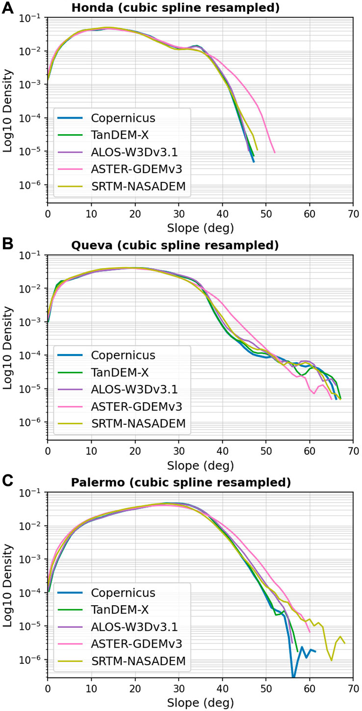
FIGURE 10. Catchment slope distributions (note the logarithmic y-axes) for each DEM in the three—(A) Honda, (B) Queva, and (C) Palermo—test catchments shown in Figure 1. Slope was calculated with the Zevenbergen and Thorne (1987) algorithm on cubic spline resampled 30-m DEMs (but results are comparable with other resampling methods). Note that the ASTER-GDEMv3, which has low inter-pixel consistency, tends to higher occurrences at higher slopes since there is greater variability in adjacent pixels.

To further investigate the impact on the slope distribution, we use percentile-percentile plots (a.k.a. QQ plots) of the 1st–99th percentile slope values of the 30-m reprojected Copernicus DEM versus the TanDEM-X, ALOS-W3Dv3.1, ASTER-GDEMv3, and SRTM-NASADEM (Figure 11). In this case, we combine the measurements for all three catchments, as the individual catchment plots showed similar relationships (Supplementary Figures S3–S5), and Figure 11 presents an average of this. We note that the Zevenbergen and Thorne (1987) algorithm takes the gradient from adjacent (edges touching) pixels for slope calculations. In the Supplementary Figure S6, we also use the Horn (1981) algorithm, which considers the diagonally adjacent (corners touching) pixels, and may be more appropriate for rougher surfaces. In Supplementary Figure S6, we note that the alternative slope calculation only reduces the magnitude of measured slopes (e.g., lower median and upper percentiles compared to Zevenbergen and Thorne (1987)), but does not change the relationship between DEMs.

FIGURE 11

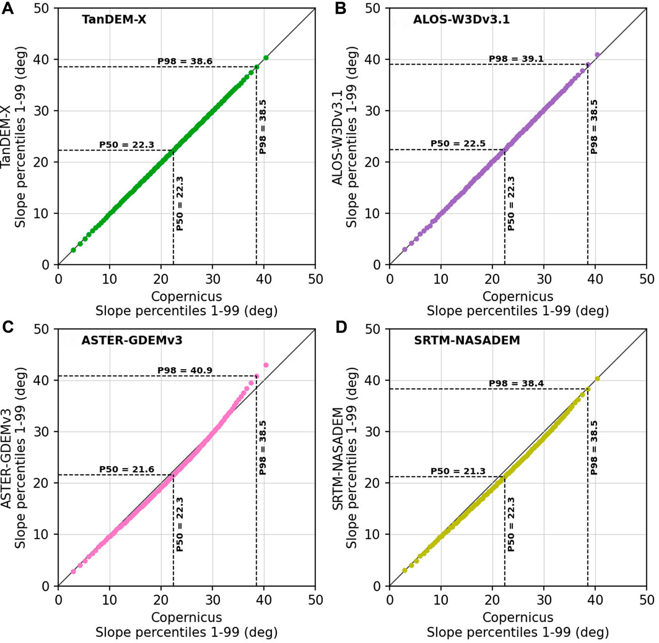
FIGURE 11. Catchment slope percentile-percentile plots on cubic spline resampled 30-m DEMs. All three slope distributions for the three test catchments (Figure 1) are combined, with separate plots for each catchment shown in Supplementary Figures S3–S5. Percentiles are compared against Copernicus (x-axis on all plots) for (A) TanDEM-X, (B) ALOS-W3Dv3.1, (C) ASTER-GDEMv3, and (D) SRTM-NASADEM. The maximum relative percentage difference in slope compared to Copernicus approaches 0.3, 1.5, 6.2, and 4.5% for the TanDEM-X, ALOS-W3Dv3.1, ASTER-GDEMv3, and SRTM-NASADEM, respectively. Slope was calculated with the Zevenbergen and Thorne (1987) algorithm, and Supplementary Figure S6 presents the results using the alternative Horn (1981) algorithm.

Figure 11 shows that the TanDEM-X distribution is nearly identical to the Copernicus, and the ALOS-W3Dv3.1 has differences of <1° at a given percentile (although often <0.5°). On the other hand, the ASTER-GDEMv3 and SRTM-NASADEM significantly diverge from the Copernicus distribution, with many ≥1° differences, and consistent under-representation of the median, and, in the case of ASTER-GDEMv3, over-representation of the upper (≥95th) percentiles. Therefore, studies relying on hillslope distributions from the ASTER and SRTM DEMs will likely under-estimate the central distribution (median) and over-estimate the tail (steepest topography), which may impact conclusions of hillslope responses to changes in erosion (e.g., Ouimet et al., 2009).

7.4.2 Channel Gradients

The inter-pixel consistency investigation is extended to the channel network in Figure 12. This plot only shows the results for the 30 m cubic-spline resampled Copernicus, ASTER-GDEMv3, and SRTM-NASADEM in the Honda catchment, and other DEMs (TanDEM-X and ALOS-W3Dv3.1) and catchments (Queva and Palermo) are provided in the Supplementary Figures S7–S11). The normalized channel steepness (k_sn) values show consistent spatial patterns in the trunk stream no matter the DEM used, with a prominent knickpoint (k_sn > 200 m^0.9) consistently around 5-km flow distance. The k_sn calculation in other catchments is generally consistent, although we do note differences for more subtle, lower-magnitude possible knickpoints in the downstream Palermo profile (Supplementary Figure S10).

FIGURE 12

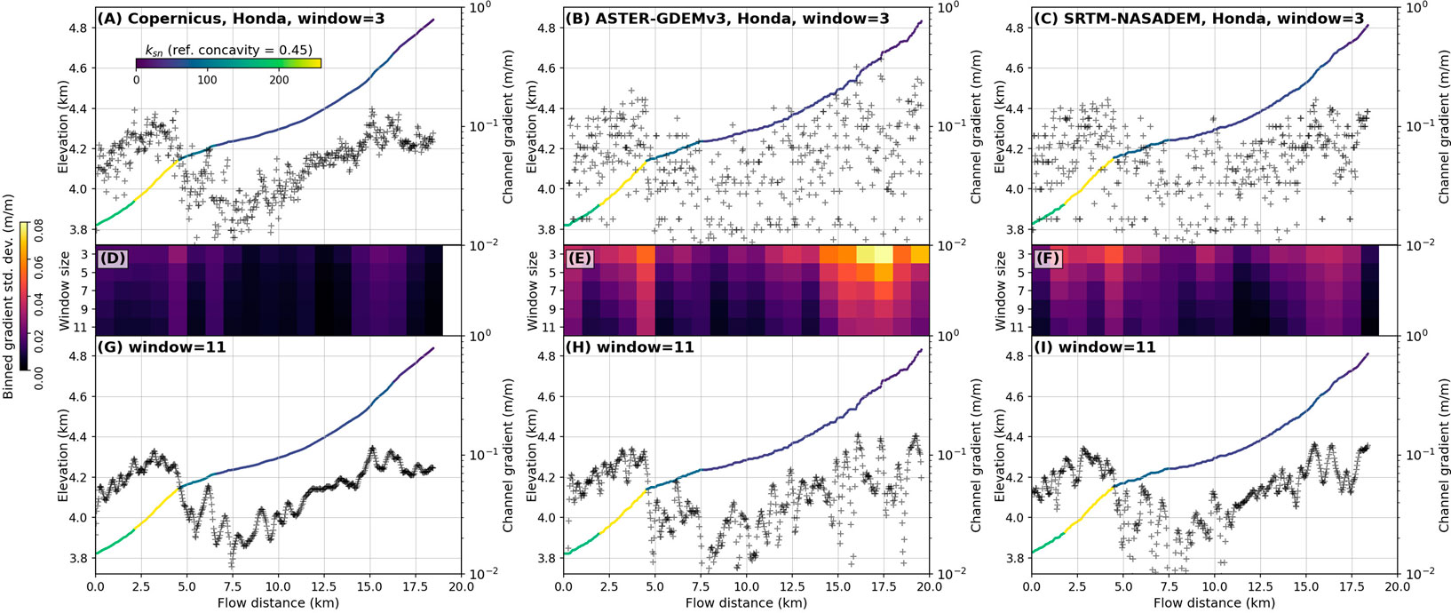
FIGURE 12. Comparison of trunk stream longitudinal river profile for the Honda Catchment (Figure 1). The left, center, and right columns correspond to the Copernicus, ASTER-GDEMv3, and SRTM-NASADEM, respectively. The top row (A–C) shows the channel elevation profile (left axis) with the channel nodes colored by their k_sn value, and the channel gradient plotted as black crosses (right axis) calculated from 3-node distances (∼90 m). The middle row (D–F) shows the standard deviation of the gradient in 1-km flow distance bins, where the first row in these sub-plots correspond to the window used in (A–C). The decrease in gradient standard deviation with increasing window size is shown in (D–F), with the last row of these sub-plots corresponding to the last row (G–I) of the figure, which shows the resulting gradient calculation using an 11-node (∼330 m) window. Other DEMs (TanDEM-X and ALOS-W3Dv3.1) and catchments (Queva and Palermo) are shown in Supplementary Figures S7–S11.

The channel steepness profile analysis is a metric usually applied to length scales of several hundred meters or longer and thus performs inherent smoothing of the input DEM data. This mitigates some effects of DEMs with large inter-pixel inconsistencies (e.g., Wobus et al., 2006). Therefore, the consistent performance of the k_sn metric is expected, and our previous work (Purinton and Bookhagen, 2017) showed similar concavity measurements using a similar range of DEMs (and DEM resolutions). We argue that for river-profile steepness analysis over several-km flow lengths in steep mountains, where the rivers descend hundreds to thousands of m in elevation, the tested DEMs perform similarly. However, we note that higher-resolution DEMs (e.g., lidar) lead to more measurements and allow finer-scaled distinction of geomorphic processes (Grieve et al., 2016; Clubb et al., 2019), although higher-resolution data require higher precision (Smith et al., 2019). This is important for detection of high magnitude, but short length-scale slope changes in river profiles, for example for knickpoint and step-pool detection.

The similarity in k_sn is not matched by the patterns of local (channel node to channel node) gradient shown in Figure 12. The 1-km binned standard deviation of gradient in the middle row (Figures 12D–F), shows a greater spread for the DEMs with lower inter-pixel consistency (ASTER-GDEMv3 and SRTM-NASADEM). As the window size of the gradient calculation is increased from three channel nodes (∼90 m) to 11 channel nodes (∼330 m), this variability is reduced (i.e., the calculation is smoothed) and the final gradients in the bottom row (Figures 12G–I) begin to resemble one another, although with clear differences remaining. Although the channel gradient calculation is smoothed with increasing window size, this comes at the cost of finer-scale analysis of slope differences in shorter (<330 m) channel reaches.

The differences in longitudinal river profile gradient calculations between the different DEMs are summarized in Figure 13. This combines all data from the three catchment trunk streams and DEMs (similar to Figure 11). Figure 13A demonstrates that the DEMs with low inter-pixel consistency (ASTER-GDEMv3 and SRTM-NASADEM) have higher variability in gradient (measured as the sum of standard deviations across all 1-km bins), but this variability converges towards the Copernicus and TanDEM-X values with increasing window size. The variability in gradient for the SRTM-NASADEM and ASTER-GDEMv3 converges on the 3-node window value of the smoother DEMs with pixel windows of 5 and 9, respectively. This implies that a DEM with lower inter-pixel consistency should use different (larger) window sizes for channel gradient calculations than a more internally consistent DEM.

FIGURE 13

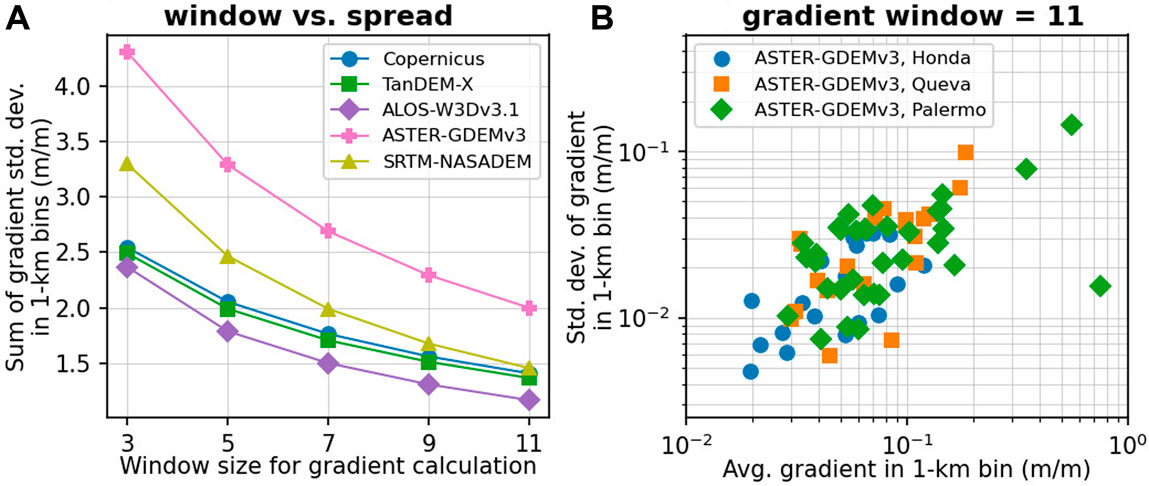
FIGURE 13. Summary window size versus gradient standard deviation for all trunk stream river profiles. (A) Sum of the gradient standard deviations across all 1-km flow distance bins in each catchment for each DEM. Note that the DEM with the lowest inter-pixel consistency (ASTER-GDEMv3, pink) shows the strongest smoothing effect with increasing window size. But even with an 11-node window smoothing, the standard deviation is 30–50% higher than for the other DEMs. Smoothing of the SRTM-NASADEM (yellow) leads to near convergence of standard deviations with the Copernicus DEM. The ALOS-W3Dv3.1 (purple) is overall smoother, potentially due to a hydrologic preconditioning step. (B) Relationship between standard deviation of gradient and average channel gradient in each 1-km flow distance bin for all three catchments for ASTER-GDEMv3, with gradient calculated in an 11-node window. Higher gradients have higher standard deviation, suggesting that higher gradients have lower inter-pixel consistencies.

Figure 13B shows another subtlety of the channel gradient analysis. Here, we see that the variability in channel gradient increases with increasing average gradient, which means that steeper parts of the channel are expected to have a greater spread of steepness. This is exactly the nature of a concave channel profile, where gradient decreases quasi-exponentially downstream (the values change more in the upper, steeper reaches). Thus, the window size of slope calculation will impact different channel reaches differently, which may be an important consideration over long or very steep profiles. Recent work has explored the usage of adaptive approaches with smoothing adjusted to the amount of slope variability (Schwanghart and Scherler, 2017; Gailleton et al., 2019).

7.5 DEM Quality and Suggestions

One interesting consideration from the analysis concerns the ALOS-W3Dv3.1. In Figure 8, the inter-pixel consistency is lower than for the Copernicus (higher percentage of power at 42- to <60-m wavelengths). However, the slope distributions are very similar to the Copernicus DEM (Figure 11B), compared to the ASTER-GDEMv3 and SRTM-NASADEM, which have much lower inter-pixel consistency (>∼10% in Figure 8). Notably, despite the lower inter-pixel consistency implied by the boxplot in Figure 8, the ALOS-W3Dv3.1 has the lowest variability in channel gradient of all DEMs (Figure 13A). This is a possible sign of a hydrologic preconditioning step of this dataset, though unreported in the technical documentation (EORC, 2021).

Although longitudinal river profile analysis at large (several km) scales in steep, high-relief catchments for tectonic and climatic forcings are less affected by DEM choice (e.g., k_sn), other catchment analysis like slope distributions will be impacted by this choice. Furthermore, fine-scale analysis of channel gradients will be particularly impacted by the channel-node to channel-node variability, with implications for assessing reach-scale channel morphology and knickpoint detection for tectonic geomorphology (e.g., Neely et al., 2017; Clubb et al., 2019; Gailleton et al., 2019) and river ecology (e.g., Beechie and Sibley, 1997; Bisson et al., 2017), among others.

This study does not address DEMs of different resolution, as we focus only on the widely used and open-source (near) global 30 m DEMs. We do note that DEM resolution will impact geomorphic analysis and the calculation of derivatives of elevation (Purinton and Bookhagen, 2017; Grieve et al., 2016; Smith et al., 2019), but many studies in remote or extensive areas will continue to rely on the 30-m datasets. Although the spatial resolution of these DEMs is too coarse for channel-head detection (e.g., Passalacqua et al., 2010a,b; Clubb et al., 2014; Hooshyar et al., 2016), high inter-pixel consistency, especially in low slopes near drainage divides, will allow more accurate flow path derivation using divergent flow routing algorithms like D∞ (Tarboton, 2005). This is an important component in soil mantled and diffusional landscapes, irrespective of vegetation cover.

Previous work to quantify vertical error in DEMs (e.g., Becek, 2008; Becek, 2014; Becek et al., 2016; Yamazaki et al., 2017) highlights that error can be introduced by various sensor biases, quantization of elevation values (i.e., integer versus floating point), and land cover. In our study, a primary goal is to avoid reference data and develop an internal metric to compare DEM quality using only a priori knowledge of a smooth, bare-earth study area with mixed steep and flat terrain. While the methods developed by Becek (2008) demonstrate a novel use of airplane runways as continuous reference surfaces, this is limited to flat terrain of limited spatial extent and requires some assumptions, such as a uniform distribution of quantization and slope-induce errors. In any case, the results from the runway method on SRTM (Becek, 2008), ASTER GDEM (Becek, 2014), and WorldDEM^TM (Becek et al., 2016) support the relative quality between these datasets found in this study (where we use the Copernicus DEM based on the WorldDEM^TM).

Technical documentation available for spaceborne DEMs (Wessel, 2016; Abrams and Crippen, 2019; Buckley et al., 2020; Leister-Taylor et al., 2020; EORC, 2021; Zink et al., 2021) contain important information on processing and limitations, but this information is often neglected and end users of 30 m DEMs require fundamental metrics of DEM quality beyond vertical point-based accuracy. Our local pixel variability metric based directly on the hillshade image (which includes slope and aspect information), combined with quantification of inter-pixel consistency and demonstration of the impacts on geomorphic research, provides a quantitative explanation of spaceborne DEM quality.

From our analysis, it is clear that the newly released Copernicus DEM—based on the high-quality TanDEM-X derived WorldDEM^TM—has the highest inter-pixel consistency, and therefore most realistic representation of the topography in our study area. This is in agreement with the findings of other studies comparing TanDEM-X to previous DEMs (Pipaud et al., 2015; Purinton and Bookhagen, 2017; Boulton and Stokes, 2018; Grohmann, 2018), and recent reporting on Copernicus (Guth and Geoffroy, 2021). We do note that other authors have found better performance of the ALOS-W3D for stream profile analysis (Schwanghart and Scherler, 2017), possibly due to hydrologic preconditioning. Older DEMs like the SRTM-NASADEM and ASTER-GDEMv3 continue to be developed, and these can be useful as time-shots of the Earth surface during collection, but geomorphic analysis at the catchment and mountain belt scale should increasingly rely on the newer Copernicus and TanDEM-X global DEMs.

8 Conclusion

This study compared the most updated versions of five (near) global DEMs with 1 arcsec (∼30 m) resolution. In order of release date for their original versions, these are the SRTM-NASADEM, ASTER-GDEMv3, ALOS-W3Dv3.1, TanDEM-X, and Copernicus DEMs. Four of these are fully open-access, while the TanDEM-X is a research-grade product available through a DLR proposal. Our study area in the steep Central Andes is geomorphically smooth and arid (nearly vegetation-free), which results in ideal conditions for bare-earth remote sensing and comparison of DEMs.

We developed new metrics for assessing vertical uncertainty that highlight the vertical variability in adjacent pixels, which is not related to true topographic signal, but rather sensor, orbital, and/or processing, including resampling, artifacts. We refer to this as the inter-pixel consistency, where low (high) inter-pixel consistency refers to high (low) variability in adjacent pixels. Our chosen analysis metric is based on high-pass filtering of the hillshade images for each DEM and does not rely on reference data. We quantified the inter-pixel consistency at greater than 2-pixel wavelengths and in adjacent pixel neighborhoods (3 × 3 pixel) using Fourier frequency analysis. We found:

1) The Copernicus DEM, which is derived from the TanDEM-X original data, has the most realistic height representation with low pixel-to-pixel noise and no longer-wavelength (≥2 pixels, or ≥ ∼60 m) artifacts.

2) The SRTM-NASADEM and ASTER-GDEMv3 contain longer-wavelength artifacts at ∼2–24 pixel (∼60–720 m) wavelengths related to sensor, orbital, and/or processing artifacts. These DEMs also contain significant high-frequency variability in adjacent pixel steps, detrimental to pixel neighborhood calculations, such as hillslope angle and channel gradient.

3) The ALOS-W3Dv3.1 may be suitable for hydrologic analysis but should be treated with care due to a 3-pixel wavelength resampling error and possible additional unreported filtering steps that affect valley bottoms.

4) DEMs with lower inter-pixel consistency (higher vertical variability) have catchment-wide slope distributions skewed to higher slope values, particularly the ASTER-GDEMv3.

5) DEMs with lower inter-pixel consistency also show higher scattering of elevation and channel gradient values in longitudinal river profiles, but these gradients can be partially smoothed by calculations using larger windows.

6) The resampling scheme that provides the most smoothing of adjacent pixel variability was cubic spline, whereas commonly used bilinear and nearest neighbor schemes provided less smooth results.

The caveat of larger window sizes or different resampling schemes is that true topographic variability is likely smoothed along with artifact variability. Therefore, the selection of a DEM with the most consistent height representation (i.e., Copernicus and TanDEM-X) is most important for quantitative geomorphic analysis. A more complete picture of DEM quality for geomorphic analysis includes pixel variability quantified with respect to local neighborhoods, beyond point-based vertical accuracy from reference data.

Data Availability Statement

Publicly available datasets were analyzed in this study. These data can be found here: https://lpdaac.usgs.gov/products/nasadem_hgtv001; https://lpdaac.usgs.gov/products/astgtmv003/; https://www.eorc.jaxa.jp/ALOS/en/aw3d30/index.htm; https://tandemx-science.dlr.de/ (available through research proposal); https://panda.copernicus.eu/web/cds-catalogue/panda.

Author Contributions

BB and BP defined the project. BP and BB developed the algorithms and BP performed all coding. BP carried out the analysis and lead the manuscript writing with input from BB. BB provided funding.

Funding

TanDEM-X DEMs were received through grant DEM_CALVAL1028 to BP through the DLR. Additional funding was sourced from DFG BO 2933/3-1 (BB), DFG funded IRTG-StRATEGy (IGK 2018) to MR Strecker and BB, and BMBF LIDAR and NEXUS funded through the MWFK Brandenburg, Germany, both for BB. We acknowledge the support of the Open Access Publishing Fund of the University of Potsdam.

Conflict of Interest

The authors declare that the research was conducted in the absence of any commercial or financial relationships that could be construed as a potential conflict of interest.

Publisher’s Note

All claims expressed in this article are solely those of the authors and do not necessarily represent those of their affiliated organizations, or those of the publisher, the editors and the reviewers. Any product that may be evaluated in this article, or claim that may be made by its manufacturer, is not guaranteed or endorsed by the publisher.

Acknowledgments

Stefanie Tofelde, Taylor Smith, Ariane Mueting, Aljoscha Rheinwalt, and the rest of the Geological Remote Sensing group at the University of Potsdam are thanked for conversations and suggestions, particularly with regards to terminology.

Supplementary Material

The Supplementary Material for this article can be found online at: https://www.frontiersin.org/articles/10.3389/feart.2021.758606/full#supplementary-material

References

Abrams, M., and Crippen, R. (2019). ASTER GDEM V3 (ASTER Global DEM) User Guide Version 1. Pasadena, CA, USA: Califronia Institute of Technology. Available at: https://lpdaac.usgs.gov/documents/434/ASTGTM_User_Guide_V3.pdf (Accessed September 23, 2021).

Google Scholar

Abrams, M., Crippen, R., and Fujisada, H. (2020). Aster Global Digital Elevation Model (Gdem) and Aster Global Water Body Dataset (Astwbd). Remote Sensing 12, 1156. doi:10.3390/rs12071156

CrossRef Full Text | Google Scholar

Allmendinger, R. W., Jordan, T. E., Kay, S. M., and Isacks, B. L. (1997). The Evolution of the Altiplano-Puna Plateau of the Central Andes. Annu. Rev. Earth Planet. Sci. 25, 139–174. doi:10.1146/annurev.earth.25.1.139

CrossRef Full Text | Google Scholar

Alonso, R. N., Jordan, T. E., Tabbutt, K. T., and Vandervoort, D. S. (1991). Giant Evaporite Belts of the Neogene central andes. Geol. 19, 401–404. doi:10.1130/0091-7613(1991)019<0401:gebotn>2.3.co;2

CrossRef Full Text | Google Scholar

Arrell, K., Wise, S., Wood, J., and Donoghue, D. (2008). Spectral Filtering as a Method of Visualising and Removing Striped Artefacts in Digital Elevation Data. Earth Surf. Process. Landforms 33, 943–961. doi:10.1002/esp.1597

CrossRef Full Text | Google Scholar

Aster, G. V. T. (2009). ASTER Global DEM Validation Summary Report. Tech. rep.. Available at: https://lpdaac.usgs.gov/documents/28/ASTER_GDEM_Validation_1_Summary_Report.pdf (Accessed September 23, 2021)

Google Scholar

Baade, J., and Schmullius, C. (2016). TanDEM-x IDEM Precision and Accuracy Assessment Based on a Large Assembly of Differential GNSS Measurements in Kruger national park, south africa. ISPRS J. Photogrammetry Remote Sensing 119, 496–508. doi:10.1016/j.isprsjprs.2016.05.005

CrossRef Full Text | Google Scholar

Bagnardi, M., González, P. J., and Hooper, A. (2016). High-resolution Digital Elevation Model from Tri-stereo Pleiades-1 Satellite Imagery for Lava Flow Volume Estimates at Fogo Volcano. Geophys. Res. Lett. 43, 6267–6275. doi:10.1002/2016gl069457

CrossRef Full Text | Google Scholar

Becek, K. (2014). Assessing Global Digital Elevation Models Using the Runway Method: The Advanced Spaceborne thermal Emission and Reflection Radiometer versus the Shuttle Radar Topography mission Case. IEEE Trans. Geosci. Remote Sensing 52, 4823–4831. doi:10.1109/TGRS.2013.2285187

CrossRef Full Text | Google Scholar

Becek, K. (2008). Investigating Error Structure of Shuttle Radar Topography mission Elevation Data Product. Geophys. Res. Lett. 35, 1. doi:10.1029/2008GL034592

CrossRef Full Text | Google Scholar

Becek, K., Koppe, W., and Kutoğlu, Ş. (2016). Evaluation of Vertical Accuracy of the WorldDEM Using the Runway Method. Remote Sensing 8, 934. doi:10.3390/rs8110934

CrossRef Full Text | Google Scholar

Beechie, T. J., and Sibley, T. H. (1997). Relationships between Channel Characteristics, Woody Debris, and Fish Habitat in Northwestern washington Streams. Trans. Am. Fish. Soc. 126, 217–229. doi:10.1577/1548-8659(1997)126<0217:rbccwd>2.3.co;2

CrossRef Full Text | Google Scholar

Bessette-Kirton, E. K., Coe, J. A., and Zhou, W. (2018). Using Stereo Satellite Imagery to Account for Ablation, Entrainment, and Compaction in Volume Calculations for Rock Avalanches on Glaciers: Application to the 2016 Lamplugh Rock Avalanche in Glacier bay national park, alaska. J. Geophys. Res. Earth Surf. 123, 622–641. doi:10.1002/2017JF004512

CrossRef Full Text | Google Scholar

Beyer, R. A., Alexandrov, O., and McMichael, S. (2018). The Ames Stereo Pipeline: NASA's Open Source Software for Deriving and Processing Terrain Data. Earth Space Sci. 5, 537–548. doi:10.1029/2018EA000409

CrossRef Full Text | Google Scholar

Bisson, P. A., Montgomery, D. R., and Buffington, J. M. (2017). “Valley Segments, Stream Reaches, and Channel Units,” in Methods in Stream Ecology, Volume 1 (Elsevier), 21–47. doi:10.1016/b978-0-12-416558-8.00002-0

CrossRef Full Text | Google Scholar

Bookhagen, B., Haselton, K., and Trauth, M. H. (2001). Hydrological Modelling of a Pleistocene Landslide-Dammed lake in the santa maria basin, NW argentina. Palaeogeogr. Palaeoclimatol. Palaeoecol. 169, 113–127. doi:10.1016/s0031-0182(01)00221-8

CrossRef Full Text | Google Scholar

Bookhagen, B., and Strecker, M. R. (2008). Orographic Barriers, High-Resolution TRMM Rainfall, and Relief Variations along the Eastern andes. Geophys. Res. Lett. 35, 1. doi:10.1029/2007gl032011

CrossRef Full Text | Google Scholar

Bookhagen, B., and Strecker, M. R. (2012). Spatiotemporal Trends in Erosion Rates across a Pronounced Rainfall Gradient: Examples from the Southern central andes. Earth Planet. Sci. Lett. 327-328, 97–110. doi:10.1016/j.epsl.2012.02.005

CrossRef Full Text | Google Scholar

Booth, A. M., Roering, J. J., and Perron, J. T. (2009). Automated Landslide Mapping Using Spectral Analysis and High-Resolution Topographic Data: Puget Sound Lowlands, washington, and portland hills, oregon. Geomorphology 109, 132–147. doi:10.1016/j.geomorph.2009.02.027

CrossRef Full Text | Google Scholar

Boulton, S. J., and Stokes, M. (2018). Which Dem Is Best for Analyzing Fluvial Landscape Development in Mountainous Terrains? Geomorphology 310, 168–187. doi:10.1016/j.geomorph.2018.03.002

CrossRef Full Text | Google Scholar

Buckley, S., Agram, P., Belz, J., Crippen, R. E., Gurrola, E. M., Hensley, S., et al. (2020). NASADEM User Guide Version 1. Pasadena, Calfironia, USA: Califronia Institute of Technology. Available at: https://lpdaac.usgs.gov/documents/592/NASADEM_User_Guide_V1.pdf (Accessed September 23, 2021).

Google Scholar

Carabajal, C. C., and Boy, J.-P. (2020). Icesat-2 Altimetry as Geodetic Control. Int. Arch. Photogramm. Remote Sens. Spat. Inf. Sci. XLIII-B3-2020, 1299–1306. doi:10.5194/isprs-archives-XLIII-B3-2020-1299-2020

CrossRef Full Text | Google Scholar

Carabajal, C. C., and Harding, D. J. (2006). Srtm C-Band and Icesat Laser Altimetry Elevation Comparisons as a Function of Tree Cover and Relief. Photogramm Eng. Remote Sensing 72, 287–298. doi:10.14358/pers.72.3.287

CrossRef Full Text | Google Scholar

Clubb, F. J., Bookhagen, B., and Rheinwalt, A. (2019). Clustering River Profiles to Classify Geomorphic Domains. J. Geophys. Res. Earth Surf. 124, 1417–1439. doi:10.1029/2019JF005025

CrossRef Full Text | Google Scholar

Clubb, F. J., Mudd, S. M., Milodowski, D. T., Hurst, M. D., and Slater, L. J. (2014). Objective Extraction of Channel Heads from High-Resolution Topographic Data. Water Resour. Res. 50, 4283–4304. doi:10.1002/2013wr015167

CrossRef Full Text | Google Scholar

Cook, K. L. (2017). An Evaluation of the Effectiveness of Low-Cost Uavs and Structure from Motion for Geomorphic Change Detection. Geomorphology 278, 195–208. doi:10.1016/j.geomorph.2016.11.009

CrossRef Full Text | Google Scholar

Crippen, R., Buckley, S., Agram, P., Belz, E., Gurrola, E., Hensley, S., et al. (2016). Nasadem Global Elevation Model: Methods and Progress. Int. Arch. Photogramm. Remote Sens. Spat. Inf. Sci. XLI-B4, 125–128. doi:10.5194/isprsarchives-xli-b4-125-2016

CrossRef Full Text | Google Scholar

Eltner, A., Kaiser, A., Castillo, C., Rock, G., Neugirg, F., and Abellán, A. (2016). Image-based Surface Reconstruction in Geomorphometry - Merits, Limits and Developments. Earth Surf. Dynam. 4, 359–389. doi:10.5194/esurf-4-359-2016

CrossRef Full Text | Google Scholar

Eorc, J. (2021). “ALOS World 3D-30m (AW3D30),” in Product Description Edition 1.2 Version 3.2/3.1 (Tech. rep., Japan Aerospace Exploration Agency). Available at: https://www.eorc.jaxa.jp/ALOS/en/aw3d30/aw3d30v3.2_product_e_e1.2.pdf (Accessed September 23, 2021).

Google Scholar

Fahrland, E., Jacob, P., Schrader, H., and Kahabka, H. (2020). Copernicus Digital Elevation Model Validation Report. Tech. Rep. GEO.2018-1988-2, AIRBUS. Available at: https://spacedata.copernicus.eu/documents/20126/0/GEO1988-CopernicusDEM-SPE-002_ProductHandbook_I1.00.pdf (Accessed September 23, 2021).

Google Scholar

Farr, T. G., Rosen, P. A., Caro, E., Crippen, R., Duren, R., Hensley, S., et al. (2007). The Shuttle Radar Topography mission. Rev. Geophys. 45, 1. doi:10.1029/2005rg000183

CrossRef Full Text | Google Scholar

Gailleton, B., Mudd, S. M., Clubb, F. J., Peifer, D., and Hurst, M. D. (2019). A Segmentation Approach for the Reproducible Extraction and Quantification of Knickpoints from River Long Profiles. Earth Surf. Dynam. 7, 211–230. doi:10.5194/esurf-7-211-2019

CrossRef Full Text | Google Scholar

Gallant, J., and Read, A. (2009). Enhancing the Srtm Data for australia. Proc. Geomorphometry 31, 149–154.

Google Scholar

GDAL/OGR contributors (2021). GDAL/OGR Geospatial Data Abstraction Software Library. Open Source Geospatial Foundation. Available at: https://gdal.org/ (Accessed September 23, 2021).

Google Scholar

Godfrey, L. V., Chan, L.-H., Alonso, R. N., Lowenstein, T. K., McDonough, W. F., Houston, J., et al. (2013). The Role of Climate in the Accumulation of Lithium-Rich Brine in the central andes. Appl. Geochem. 38, 92–102. doi:10.1016/j.apgeochem.2013.09.002

CrossRef Full Text | Google Scholar

González, C., Bachmann, M., Bueso-Bello, J.-L., Rizzoli, P., and Zink, M. (2020). A Fully Automatic Algorithm for Editing the Tandem-X Global Dem. Remote Sensing 12, 3961. doi:10.3390/rs12233961

CrossRef Full Text | Google Scholar

Grieve, S. W. D., Mudd, S. M., Milodowski, D. T., Clubb, F. J., and Furbish, D. J. (2016). How Does Grid-Resolution Modulate the Topographic Expression of Geomorphic Processes? Earth Surf. Dynam. 4, 627–653. doi:10.5194/esurf-4-627-2016

CrossRef Full Text | Google Scholar

Grohmann, C. H. (2018). Evaluation of Tandem-X Dems on Selected Brazilian Sites: Comparison with Srtm, Aster Gdem and Alos Aw3d30. Remote Sensing Environ. 212, 121–133. doi:10.1016/j.rse.2018.04.043

CrossRef Full Text | Google Scholar

Guth, P. L., and Geoffroy, T. M. (2021). LiDAR point Cloud and ICESat‐2 Evaluation of 1 Second Global Digital Elevation Models: Copernicus Wins. Trans. GIS 406, 1–17. doi:10.1111/tgis.12825

CrossRef Full Text | Google Scholar

Hain, M. P., Strecker, M. R., Bookhagen, B., Alonso, R. N., Pingel, H., and Schmitt, A. K. (2011). Neogene to Quaternary Broken Foreland Formation and Sedimentation Dynamics in the andes of Nw argentina (25°s). Tectonics 30, 2. doi:10.1029/2010tc002703

CrossRef Full Text | Google Scholar

Haselton, K., Hilley, G., and Strecker, M. R. (2002). Average Pleistocene Climatic Patterns in the Southern central andes: Controls on Mountain Glaciation and Paleoclimate Implications. J. Geology. 110, 211–226. doi:10.1086/338414

CrossRef Full Text | Google Scholar

Hawker, L., Bates, P., Neal, J., and Rougier, J. (2018). Perspectives on Digital Elevation Model (Dem) Simulation for Flood Modeling in the Absence of a High-Accuracy Open Access Global Dem. Front. Earth Sci. 6, 233. doi:10.3389/feart.2018.00233

CrossRef Full Text | Google Scholar

Hofton, M., Dubayah, R., Blair, J. B., and Rabine, D. (2006). Validation of SRTM Elevations over Vegetated and Non-vegetated Terrain Using Medium Footprint Lidar. Photogramm Eng. Remote Sensing 72, 279–285. doi:10.14358/pers.72.3.279

CrossRef Full Text | Google Scholar

Hooshyar, M., Katul, G., and Porporato, A. (2021). Spectral Signature of Landscape Channelization. Geophys. Res. Lett. 48, e2020GL091015. E2020GL091015 2020GL091015. doi:10.1029/2020GL091015

CrossRef Full Text | Google Scholar

Hooshyar, M., Wang, D., Kim, S., Medeiros, S. C., and Hagen, S. C. (2016). Valley and Channel Networks Extraction Based on Local Topographic Curvature Andk-Means Clustering of Contours. Water Resour. Res. 52, 8081–8102. doi:10.1002/2015wr018479

CrossRef Full Text | Google Scholar

Horn, B. K. P. (1981). Hill Shading and the Reflectance Map. Proc. IEEE 69, 14–47. doi:10.1109/PROC.1981.11918

CrossRef Full Text | Google Scholar

Huete, A., Justice, C., and Liu, H. (1994). Development of Vegetation and Soil Indices for Modis-Eos. Remote Sensing Environ. 49, 224–234. doi:10.1016/0034-4257(94)90018-3

CrossRef Full Text | Google Scholar

Hurst, M. D., Mudd, S. M., Walcott, R., Attal, M., and Yoo, K. (2012). Using Hilltop Curvature to Derive the Spatial Distribution of Erosion Rates. J. Geophys. Res. 117, a–n. doi:10.1029/2011JF002057

CrossRef Full Text | Google Scholar

Jarvis, A., Reuter, H. I., Nelson, A., and Guevara, E. (2008). Hole-filled Srtm for the globe Version 4. Available from the CGIAR-CSI SRTM 90m Database. Available at: http://srtm.csi.cgiar.org/.

Google Scholar

Kääb, A. (2002). Monitoring High-Mountain Terrain Deformation from Repeated Air- and Spaceborne Optical Data: Examples Using Digital Aerial Imagery and Aster Data. ISPRS J. Photogrammetry Remote Sensing 57, 39–52. doi:10.1016/S0924-2716(02)00114-4

CrossRef Full Text | Google Scholar

Kramm, T., and Hoffmeister, D. (2019). A Relief Dependent Evaluation of Digital Elevation Models on Different Scales for Northern chile. Ijgi 8, 430. doi:10.3390/ijgi8100430

CrossRef Full Text | Google Scholar

Krieger, G., Zink, M., Bachmann, M., Bräutigam, B., Schulze, D., Martone, M., et al. (2013). Tandem-x: A Radar Interferometer with Two Formation-Flying Satellites. Acta Astronautica 89, 83–98. doi:10.1016/j.actaastro.2013.03.008

CrossRef Full Text | Google Scholar

Leister-Taylor, V., Jacob, P., Schrader, H., and Kahabka, H. (2020). Copernicus Digital Elevation Model Product Handbook. Tech. Rep. GEO.2018-1988-2, AIRBUS. Available at: https://spacedata.copernicus.eu/documents/20126/0/GEO1988-CopernicusDEM-RP-001_ValidationReport_I3.0.pdf (Accessed September 23, 2021).

Google Scholar

Liu, Y., Bates, P. D., Neal, J. C., and Yamazaki, D. (2021). Bare-earth Dem Generation in Urban Areas for Flood Inundation Simulation Using Global Digital Elevation Models. Water Resour. Res. 57, e2020WR028516. E2020WR028516 2020WR028516. doi:10.1029/2020wr028516

CrossRef Full Text | Google Scholar

Luna, L. V., Bookhagen, B., Niedermann, S., Rugel, G., Scharf, A., and Merchel, S. (2018). Glacial Chronology and Production Rate Cross-Calibration of Five Cosmogenic Nuclide and mineral Systems from the Southern central Andean Plateau. Earth Planet. Sci. Lett. 500, 242–253. doi:10.1016/j.epsl.2018.07.034

CrossRef Full Text | Google Scholar

Milodowski, D. T., Mudd, S. M., and Mitchard, E. T. A. (2015). Topographic Roughness as a Signature of the Emergence of Bedrock in Eroding Landscapes. Earth Surf. Dynam. 3, 483–499. doi:10.5194/esurf-3-483-2015

CrossRef Full Text | Google Scholar

Mudd, S. M., Attal, M., Milodowski, D. T., Grieve, S. W. D., and Valters, D. A. (2014). A Statistical Framework to Quantify Spatial Variation in Channel Gradients Using the Integral Method of Channel Profile Analysis. J. Geophys. Res. Earth Surf. 119, 138–152. doi:10.1002/2013JF002981

CrossRef Full Text | Google Scholar

Mudd, S. M., Clubb, F. J., Grieve, S. W. D., Milodowski, D. T., Hurst, M. D., Gailleton, B., et al. (2019). Lsdtopotools2. doi:10.5281/zenodo.3245041

CrossRef Full Text | Google Scholar

Mudd, S. M. (2020). “Topographic Data from Satellites,” in Developments in Earth Surface Processes (Elsevier), 91–128. doi:10.1016/b978-0-444-64177-9.00004-7

CrossRef Full Text | Google Scholar

Neely, A. B., Bookhagen, B., and Burbank, D. W. (2017). An Automated Knickzone Selection Algorithm (KZ‐Picker) to Analyze Transient Landscapes: Calibration and Validation. J. Geophys. Res. Earth Surf. 122, 1236–1261. doi:10.1002/2017jf004250

CrossRef Full Text | Google Scholar

Neuenschwander, A., and Pitts, K. (2019). The Atl08 Land and Vegetation Product for the Icesat-2 mission. Remote Sensing Environ. 221, 247–259. doi:10.1016/j.rse.2018.11.005

CrossRef Full Text | Google Scholar

Nuth, C., and Kääb, A. (2011). Co-registration and Bias Corrections of Satellite Elevation Data Sets for Quantifying Glacier Thickness Change. The Cryosphere 5, 271–290. doi:10.5194/tc-5-271-2011

CrossRef Full Text | Google Scholar

O’Callaghan, J. F., and Mark, D. M. (1984). The Extraction of Drainage Networks from Digital Elevation Data. Comp. Vis. Graphics, Image Process. 28, 323–344. doi:10.1016/S0734-189X(84)80011-0

CrossRef Full Text | Google Scholar

Olen, S., and Bookhagen, B. (2020). Applications of Sar Interferometric Coherence Time Series: Spatiotemporal Dynamics of Geomorphic Transitions in the South-central andes. J. Geophys. Res. Earth Surf. 125, e2019JF005141. E2019JF005141 2019JF005141. doi:10.1029/2019JF005141

CrossRef Full Text | Google Scholar

Ouimet, W. B., Whipple, K. X., and Granger, D. E. (2009). Beyond Threshold Hillslopes: Channel Adjustment to Base-Level Fall in Tectonically Active Mountain Ranges. Geology 37, 579–582. doi:10.1130/G30013A.1

CrossRef Full Text | Google Scholar

Passalacqua, P., Belmont, P., Staley, D. M., Simley, J. D., Arrowsmith, J. R., Bode, C. A., et al. (2015). Analyzing High Resolution Topography for Advancing the Understanding of Mass and Energy Transfer through Landscapes: A Review. Earth-Science Rev. 148, 174–193. doi:10.1016/j.earscirev.2015.05.012

CrossRef Full Text | Google Scholar

Passalacqua, P., Tarolli, P., and Foufoula-Georgiou, E. (2010a). Testing Space-Scale Methodologies for Automatic Geomorphic Feature Extraction from Lidar in a Complex Mountainous Landscape. Water Resour. Res. 46, n/a. doi:10.1029/2009WR008812

CrossRef Full Text | Google Scholar

Passalacqua, P., Trung, T. D., Foufoula-Georgiou, E., Sapiro, G., and Dietrich, W. E. (2010b). A Geometric Framework for Channel Network Extraction from Lidar: Nonlinear Diffusion and Geodesic Paths. J. Geophys. Res. 115, 1. doi:10.1029/2009jf001254

CrossRef Full Text | Google Scholar

Perron, J. T., Kirchner, J. W., and Dietrich, W. E. (2008). Spectral Signatures of Characteristic Spatial Scales and Nonfractal Structure in Landscapes. J. Geophys. Res. 113, 1. doi:10.1029/2007JF000866

CrossRef Full Text | Google Scholar

Perron, J. T., and Royden, L. (2013). An Integral Approach to Bedrock River Profile Analysis. Earth Surf. Process. Landforms 38, 570–576. doi:10.1002/esp.3302

CrossRef Full Text | Google Scholar

Pingel, H., Strecker, M. R., Mulch, A., Alonso, R. N., Cottle, J., and Rohrmann, A. (2020). Late Cenozoic Topographic Evolution of the Eastern Cordillera and Puna Plateau Margin in the Southern central andes (Nw argentina). Earth Planet. Sci. Lett. 535, 116112. doi:10.1016/j.epsl.2020.116112

CrossRef Full Text | Google Scholar

Pipaud, I., Loibl, D., and Lehmkuhl, F. (2015). Evaluation of TanDEM-X Elevation Data for Geomorphological Mapping and Interpretation in High Mountain Environments - A Case Study from SE Tibet, China. Geomorphology 246, 232–254. doi:10.1016/j.geomorph.2015.06.025

CrossRef Full Text | Google Scholar

Polidori, L., and El Hage, M. (2020). Digital Elevation Model Quality Assessment Methods: A Critical Review. Remote Sensing 12, 3522. doi:10.3390/rs12213522

CrossRef Full Text | Google Scholar

Purinton, B., and Bookhagen, B. (2018). Measuring Decadal Vertical Land-Level Changes from SRTM-C (2000) and TanDEM-X (∼ 2015) in the South-central Andes. Earth Surf. Dynam. 6, 971–987. doi:10.5194/esurf-6-971-2018

CrossRef Full Text | Google Scholar

Purinton, B., and Bookhagen, B. (2020). Multiband (X, C, L) Radar Amplitude Analysis for a Mixed Sand- and Gravel-Bed River in the Eastern central andes. Remote Sensing Environ. 246, 111799. doi:10.1016/j.rse.2020.111799

CrossRef Full Text | Google Scholar

Purinton, B., and Bookhagen, B. (2017). Validation of Digital Elevation Models (Dems) and Comparison of Geomorphic Metrics on the Southern central Andean Plateau. Earth Surf. Dynam. 5, 211–237. doi:10.5194/esurf-5-211-2017

CrossRef Full Text | Google Scholar

Rexer, M., and Hirt, C. (2014). Comparison of Free High Resolution Digital Elevation Data Sets (ASTER GDEM2, SRTM v2.1/v4.1) and Validation against Accurate Heights from the Australian National Gravity Database. Aust. J. Earth Sci. 61, 213–226. doi:10.1080/08120099.2014.884983

CrossRef Full Text | Google Scholar

Rheinwalt, A., Goswami, B., and Bookhagen, B. (2019). A Network‐Based Flow Accumulation Algorithm for Point Clouds: Facet‐Flow Networks (FFNs). J. Geophys. Res. Earth Surf. 124, 2013–2033. doi:10.1029/2018jf004827

CrossRef Full Text | Google Scholar

Rignot, E., Echelmeyer, K., and Krabill, W. (2001). Penetration Depth of Interferometric Synthetic-Aperture Radar Signals in Snow and Ice. Geophys. Res. Lett. 28, 3501–3504. doi:10.1029/2000GL012484

CrossRef Full Text | Google Scholar

Rizzoli, P., Martone, M., Gonzalez, C., Wecklich, C., Borla Tridon, D., Bräutigam, B., et al. (2017). Generation and Performance Assessment of the Global Tandem-X Digital Elevation Model. ISPRS J. Photogrammetry Remote Sensing 132, 119–139. doi:10.1016/j.isprsjprs.2017.08.008

CrossRef Full Text | Google Scholar

Rodríguez, E., Morris, C. S., and Belz, J. E. (2006). A Global Assessment of the SRTM Performance. Photogramm Eng. Remote Sensing 72, 249–260. doi:10.14358/pers.72.3.249

CrossRef Full Text | Google Scholar

Roering, J. J., Mackey, B. H., Marshall, J. A., Sweeney, K. E., Deligne, N. I., Booth, A. M., et al. (2013). ‘You Are HERE’: Connecting the Dots with Airborne Lidar for Geomorphic Fieldwork. Geomorphology 200, 172–183. doi:10.1016/j.geomorph.2013.04.009

CrossRef Full Text | Google Scholar

Roering, J. J., Marshall, J., Booth, A. M., Mort, M., and Jin, Q. (2010). Evidence for Biotic Controls on Topography and Soil Production. Earth Planet. Sci. Lett. 298, 183–190. doi:10.1016/j.epsl.2010.07.040

CrossRef Full Text | Google Scholar

Rohrmann, A., Strecker, M. R., Bookhagen, B., Mulch, A., Sachse, D., Pingel, H., et al. (2014). Can Stable Isotopes Ride Out the Storms? the Role of Convection for Water Isotopes in Models, Records, and Paleoaltimetry Studies in the central andes. Earth Planet. Sci. Lett. 407, 187–195. doi:10.1016/j.epsl.2014.09.021

CrossRef Full Text | Google Scholar

Rossi, C., Minet, C., Fritz, T., Eineder, M., and Bamler, R. (2016). Temporal Monitoring of Subglacial Volcanoes with TanDEM-X - Application to the 2014-2015 Eruption within the Bárðarbunga Volcanic System, Iceland. Remote Sensing Environ. 181, 186–197. doi:10.1016/j.rse.2016.04.003

CrossRef Full Text | Google Scholar

Schumann, G. J.-P., and Bates, P. D. (2018). The Need for a High-Accuracy, Open-Access Global Dem. Front. Earth Sci. 6, 225. doi:10.3389/feart.2018.00225

CrossRef Full Text | Google Scholar

Schwanghart, W., and Scherler, D. (2017). Bumps in River Profiles: Uncertainty Assessment and Smoothing Using Quantile Regression Techniques. Earth Surf. Dynam. 5, 821–839. doi:10.5194/esurf-5-821-2017

CrossRef Full Text | Google Scholar

Schwanghart, W., and Scherler, D. (2014). Short Communication: TopoToolbox 2 - MATLAB-Based Software for Topographic Analysis and Modeling in Earth Surface Sciences. Earth Surf. Dynam. 2, 1–7. doi:10.5194/esurf-2-1-2014

CrossRef Full Text | Google Scholar

Shean, D. E., Bhushan, S., Montesano, P., Rounce, D. R., Arendt, A., and Osmanoglu, B. (2020). A Systematic, Regional Assessment of High Mountain Asia Glacier Mass Balance. Front. Earth Sci. 7, 363. doi:10.3389/feart.2019.00363

CrossRef Full Text | Google Scholar

Smith, M. W., Carrivick, J. L., and Quincey, D. J. (2015). Structure from Motion Photogrammetry in Physical Geography. Prog. Phys. Geogr. Earth Environ. 40, 247–275. doi:10.1177/0309133315615805

CrossRef Full Text | Google Scholar

Smith, T., Rheinwalt, A., and Bookhagen, B. (2019). Determining the Optimal Grid Resolution for Topographic Analysis on an Airborne Lidar Dataset. Earth Surf. Dynam. 7, 475–489. doi:10.5194/esurf-7-475-2019

CrossRef Full Text | Google Scholar

Sofia, G. (2020). Combining Geomorphometry, Feature Extraction Techniques and Earth-Surface Processes Research: The Way Forward. Geomorphology 355, 107055. doi:10.1016/j.geomorph.2020.107055

CrossRef Full Text | Google Scholar

Strecker, M. R., Alonso, R. N., Bookhagen, B., Carrapa, B., Hilley, G. E., Sobel, E. R., et al. (2007). Tectonics and Climate of the Southern central andes. Annu. Rev. Earth Planet. Sci. 35, 747–787. doi:10.1146/annurev.earth.35.031306.140158

CrossRef Full Text | Google Scholar

Struble, W. T., Roering, J. J., Dorsey, R. J., and Bendick, R. (2021). Characteristic Scales of Drainage Reorganization in Cascadia. Geophys. Res. Lett. 48, e2020GL091413. E2020GL091413 2020GL091413. doi:10.1029/2020GL091413

CrossRef Full Text | Google Scholar

Sun, G., Ranson, K. J., Kharuk, V. I., and Kovacs, K. (2003). Validation of Surface Height from Shuttle Radar Topography mission Using Shuttle Laser Altimeter. Remote Sensing Environ. 88, 401–411. doi:10.1016/j.rse.2003.09.001

CrossRef Full Text | Google Scholar

Tachikawa, T., Kaku, M., Iwasaki, A., Gesch, D. B., Oimoen, M. J., Zhang, Z., et al. (2011). ASTER Global Digital Elevation Model Version 2-summary of Validation Results. Tech. rep., NASA. Available at: http://pubs.er.usgs.gov/publication/70005960 (Accessed September 23, 2021).

Google Scholar

Tadono, T., Ishida, H., Oda, F., Naito, S., Minakawa, K., and Iwamoto, H. (2014). Precise Global DEM Generation by ALOS PRISM. ISPRS Ann. Photogramm. Remote Sens. Spat. Inf. Sci. II-4, 71–76. doi:10.5194/isprsannals-ii-4-71-2014

CrossRef Full Text | Google Scholar

Takaku, J., Tadono, T., and Tsutsui, K. (2014). Generation of High Resolution Global Dsm from Alos Prism. Int. Arch. Photogramm. Remote Sens. Spat. Inf. Sci. XL-4, 243–248. doi:10.5194/isprsarchives-xl-4-243-2014

CrossRef Full Text | Google Scholar

Tarboton, D. G. (2005). Terrain Analysis Using Digital Elevation Models (Taudem). Logan: Utah State University.

Google Scholar

Wapenhans, I., Fernandes, V. M., O’Malley, C., White, N., and Roberts, G. G. (2021). Scale-dependent Contributors to River Profile Geometry. J. Geophys. Res. Earth Surf. 126, e2020JF005879. E2020JF005879 2020JF005879. doi:10.1029/2020jf005879

CrossRef Full Text | Google Scholar

Wessel, B., Huber, M., Wohlfart, C., Marschalk, U., Kosmann, D., and Roth, A. (2018). Accuracy Assessment of the Global Tandem-X Digital Elevation Model with Gps Data. ISPRS J. Photogrammetry Remote Sensing 139, 1–12. doi:10.1016/j.isprsjprs.2018.02.017

CrossRef Full Text | Google Scholar

Wessel, B. (2016). Tandem-x Ground Segment–Dem Products Specification Document.

Google Scholar

Wobus, C., Whipple, K. X., Kirby, E., Snyder, N., Johnson, J., Spyropolou, K., et al. (2006). “Tectonics from Topography: Procedures, Promise, and Pitfalls,” in Special Paper 398: Tectonics, Climate, and Landscape Evolution (Geological Society of America), 55–74. doi:10.1130/2006.2398(04)

CrossRef Full Text | Google Scholar

Yamazaki, D., Ikeshima, D., Tawatari, R., Yamaguchi, T., O'Loughlin, F., Neal, J. C., et al. (2017). A High-Accuracy Map of Global Terrain Elevations. Geophys. Res. Lett. 44, 5844–5853. doi:10.1002/2017GL072874

CrossRef Full Text | Google Scholar

Zevenbergen, L. W., and Thorne, C. R. (1987). Quantitative Analysis of Land Surface Topography. Earth Surf. Process. Landforms 12, 47–56. doi:10.1002/esp.3290120107

CrossRef Full Text | Google Scholar

Zink, M., Moreira, A., Hajnsek, I., Rizzoli, P., Bachmann, M., Kahle, R., et al. (2021). “Tandem-x: 10 Years of Formation Flying Bistatic Sar Interferometry,” in IEEE Journal of Selected Topics in Applied Earth Observations and Remote Sensing (IEEE). doi:10.1109/jstars.2021.3062286

CrossRef Full Text | Google Scholar