Quantifying the Seawater Sulfate Concentration in the Cambrian Ocean

Although the earliest animals might have evolved in certain “sweet spots” in the last 10 million years of Ediacaran (550–541 Ma), the Cambrian explosion requires sufficiently high levels of oxygen (O₂) in the atmosphere and diverse habitable niches in the substantively oxygenated seafloor. However, previous studies indicate that the marine redox landscape was temporally oscillatory and spatially heterogeneous, suggesting the decoupling of atmospheric oxygenation and oceanic oxidation. The seawater sulfate concentration is controlled by both the atmospheric O₂ level and the marine redox condition, with sulfide oxidation in continents as the major source, and sulfate reduction and pyrite burial as the major sink of seawater sulfate. It is thus important to quantify the sulfate concentration on the eve of the Cambrian explosion. In this study, we measured the pyrite contents and pyrite sulfur isotopes of black shale samples from the Yurtus Formation (Cambrian Series 2) in the Tarim Block, northwestern China. A numerical model is developed to calculate the seawater sulfate concentration using the pyrite content and pyrite sulfur isotope data. We first calibrate some key parameters based on observations from modern marine sediments. Then, the Monte Carlo simulation is applied to reduce the uncertainty raised by loosely confined parameters. Based on the geochemical data from both Tarim and Yangtze blocks, the modeling results indicate the seawater sulfate concentration of 8.9–14 mM, suggesting the seawater sulfate concentration was already 30–50% of the present level (28 mM). High seawater sulfate concentration might be attributed to the enhanced terrestrial sulfate input and widespread ocean oxygenation on the eve of the Cambrian explosion.

Introduction

The seawater sulfate concentration is a critical indicator of the redox condition in the atmosphereocean system. On the one hand, the seawater sulfate concentration is controlled by both marine redox condition and atmospheric O₂ level, because oxidative weathering of sulfide in continents is one of the major sources, and sulfate reduction and pyrite burial represent one of the major sinks of seawater sulfate (Canfield, 2004; Canfield and Farquhar, 2009). On the other hand, the seawater sulfate concentration should be globally homogeneous, reflecting the overall global redox condition of the atmosphere-ocean system. Thus, reconstruction of seawater sulfate concentration would provide a direct constraint on the global ocean redox condition and the atmospheric O₂ level.

The second rise of atmospheric O₂ level occurred in the late Neoproterozoic, coined the Neoproterozoic oxygenation event (NOE) (Shields-Zhou and Och, 2011). NOE is supported by several lines of geochemical evidence. The enrichment of redox-sensitive elements (e.g., V, U, Mo) in the early Ediacaran black shales implies the oxidation of the deep ocean immediately after the Marinoan Snowball Earth glaciation (Sahoo et al., 2012; Sahoo et al., 2016). The global occurrence of Shuram Excursion, the largest negative carbon isotope excursion in Earth’s history, has been interpreted as massive oxidation of dissolved organic carbon (DOC) in the Ediacaran deep ocean (Fike et al., 2006; Kaufman et al., 2007; McFadden et al., 2008; Grotzinger et al., 2011). Furthermore, the decrease in the reactive Fe content in deep-sea deposits also indicates oxidation of the deep ocean after the Ediacaran Gaskiers glaciation (580 Ma) (Canfield et al., 2007). NOE was associated with the dramatic change in the biosphere. For example, biomarker data indicate the increase in eukaryotic primary productivity in the nonglacial interlude between the two Cryogenian (720–635 Ma) Snowball Earth glaciations, while paleontological data indicate the diversification of eukaryotes in the earliest Ediacaran and the subsequent evolution of multicellular organisms, e.g., macroscopic algae and Ediacara biota (Glaessner, 1984; Zhang, 1989; Narbonne, 2005; Yin et al., 2007; Yuan et al., 2011; Liu et al., 2014; Brocks et al., 2017).

Although the biological evolution and the atmosphereocean oxygenation were broadly coincident in the geochemical and paleontological records, more and more studies indicate inconsistent or even contradictory results drawn from different proxies. It is proposed that the redox landscape in the Ediacaran and early Cambrian ocean might be temporally dynamic and spatially heterogeneous (Li et al., 2010; Sahoo et al., 2016; Li et al., 2018), and the ocean was predominantly anoxic and was frequently punctuated by episodic or sporadic oxidation or euxinia (Sahoo et al., 2016; Zhang et al., 2018; Ding et al., 2019).

The seawater sulfate concentration would provide the key evidence to resolve the inconsistency between different proxies. However, the seawater sulfate concentration cannot be directly measured from sedimentary rocks. Based on the stratigraphic variation of sulfur isotopes of carbonate-associated sulfate (CAS, δ³⁴S_CAS) (Kah et al., 2004), low seawater sulfate concentration of ∼2 mM in the early Cambrian ocean was proposed (Loyd et al., 2012; Thompson and Kah, 2012). In contrast, the marine sulfur mass balance model indicates a higher seawater sulfate concentration of ∼10 mM. In the latter scenario, it is suggested that the high seawater sulfate concentration might be attributed to the invention of bioturbation during the Cambrian explosion (Canfield and Farquhar, 2009). Such contradictory results prevent further discussion of marine-atmosphere redox coupling on the eve of the Cambrian explosion.

In this study, we develop a new method to quantify the seawater sulfate concentration by using Fe speciation and pyrite sulfur isotope data. We analyzed the black shale of the lower Cambrian Yurtus Formation in the western Tarim Block, northwestern China. Combining with geochemical data from the Yangtze Block, the seawater sulfate concentration in the early Cambrian ocean was quantified.

Geological Background

The Cambrian strata in the Arksu region, western Tarim Block, consist of, in ascending order, the Yurtus (YF), Xiaoerblak (XF), Wusongger (WF), Shayilike (SF), Awatage (AF), and Qiulitage (QF) formations. The Yurtus Formation unconformably overlies the Ediacaran Qigeblak Formation and conformably underlies the Xiaoerblak Formation (Figure 1) (He et al., 2010, 2018; Zhu et al., 2018). The basal Yurtus Formation is restricted to the Tommotian (equivalent to Stage 2 of Terreneuvian Series in the Geological Time Scale) by the appearances of Asteridium-Heliosphaeridium-Comasphaeridium acritarch assemblage (Yao et al., 2005; Dong et al., 2009). Univalve mollusk fossils (Shabaktiella multiformis, Parcaconus xinjiangensis, Eoyochelcionella aksuensis, etc.) discovered from the upper Yurtus Formation might be correlated with the small shelly fossils from the Qiongzhusian strata in South China or the Atdabanian Stage in the Eastern European Platform (equivalent to Stage 3 of Cambrian Series 2 in the Geological Time Scale) (Qian, 1999; Qian et al., 2000; Gradstein et al., 2012). Furthermore, the absence of trilobite suggests that the Yurtus Formation might belong to Cambrian Stage 2 and probably predate Cambrian Stage 3, i.e., between 529 and 521 Ma (Dong et al., 2009). Samples were collected from the drill core (X1). The Yurtus Formation in the X1 core is composed of, in stratigraphic order, bedded chert (∼3.7 m), black shale (∼23 m), intercalated mudstone and dolostone (∼13 m), and dolostone (∼13 m) lithological units. In this study, only the black shale samples from the lower Yurtus Formation were analyzed.

FIGURE 1

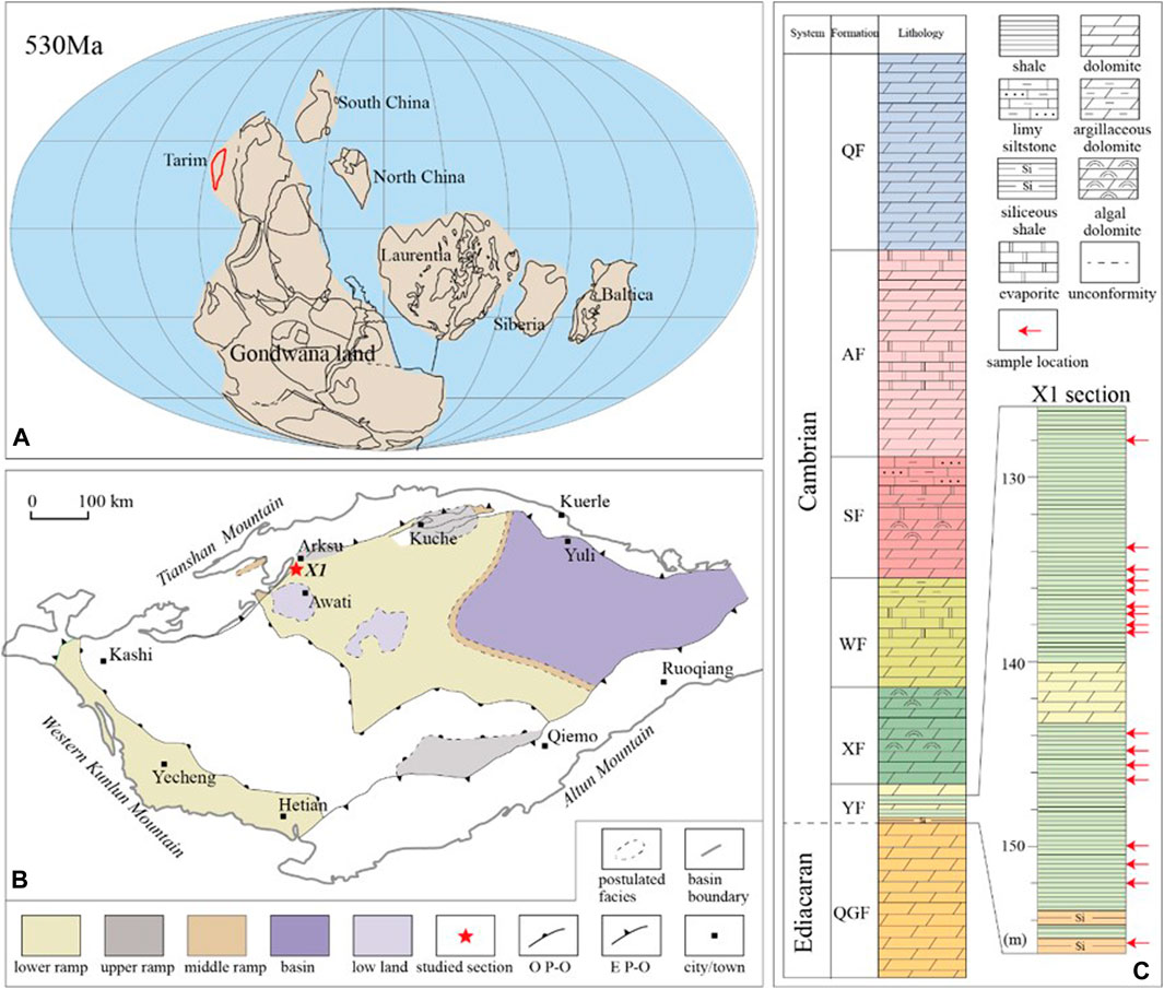
FIGURE 1. (A) Paleogeographic map of the Tarim Block during the early Cambrian (530 Ma) [modified from Li et al. (2008)]. (B) Sedimentary facies map of the early Cambrian Yurtus Formation of the Tarim Block [modified from Du and Pan (2016)] and the location of drill core XK1. O P-O= Overlapping pinch-out line of the Yurtus Formation, E P-O= Erosional pinch-out line of the Cambrian strata. (C) Stratigraphic column of the Cambrian strata in the Tarim Block [modified from Zhu et al. (2018)] and the Yurtus Formation of XK1 drill core. Red arrows indicate the stratigraphic location of samples. QGF = Qigeblak, YF = Yurtus, XF = Xiaoerblak, WF = Wusongger, SF = Shayilike, AF = Awatage, QF = Qiulitage. The depth values are relative to the top of the drill core.

Methods of Geochemical Analyses

Pyrite Sulfur Isotope Analysis

Pyrite sulfur isotope ratios were determined at the State Key Laboratory of Biogeology and Environmental Geology, China University of Geosciences (Wuhan). The purified Ag₂S precipitate (after chromium reduction) was mixed with an excessive amount of V₂O₅ and was wrapped in a tin cup. S isotope ratios were determined by a Thermo Instruments Delta V Plus isotope ratio mass spectrometer coupled with a Costech elemental analyzer. S isotope values are reported by delta notation as per mil (‰) deviation relative to the V-CDT (Vienna-Cañon Diablo Tribolite) international standard. Samples were calibrated by international standards: IAEA S1 (−0.3‰), IAEA S2 (22.65‰), and IAEA S3 (−32.5‰). The analytical precision is ∼0.1‰ (1σ), which was determined by repeated analyses of IAEA international standards.

Results

The Fe speciation and pyrite sulfur isotope data are tabulated in Table 1, and the Fe speciation data have been reported in Zhu et al. (2021). The stratigraphic profiles of geochemical data are illustrated in Figure 2. Pyrite sulfur isotope (δ³⁴S_py) ranges from -8.2‰ to +16.1‰ (mean = +4.2‰, n = 17), with most being higher than 5.0‰ in the lower black shale interval. The δ³⁴S_CAS values vary between +26.2‰ and +36.1‰ (mean = +30.4‰, n = 12). Pyrite contents range from 0.05 to 8.62% (mean = 2.26%, n = 17). These samples have wide ranges of variation of Fe_T contents, ranging from 0.49 to 4.40% (mean = 1.51%, n = 17). Fe_HR contents range between 0.25 and 4.48% (mean = 1.27, n = 17), with the maximum value at the uppermost black shale. Fe_py contents range between 0.02 and 4.02% (mean = 1.06, n = 17). The Fe_HR/Fe_T ratios vary between 0.20 and 1.00 (mean = 0.81, n = 17). Fe_py/Fe_HR ratios vary between 0.07 and 0.90 (mean = 0.75, n = 17).

TABLE 1

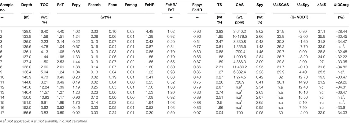
TABLE 1. Iron speciation data and pyrite sulfur isotopes of the early Cambrian Yurtus Formation in the Tarim Block.

FIGURE 2

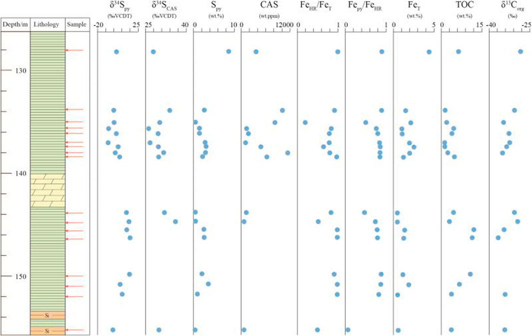
FIGURE 2. Geochemical profiles of the early Cambrian Yurtus Formation in the Tarim Block, northwestern China. Fe speciation data have been reported in Zhu et al. (2021).

Discussion

A numerical model was developed to simulate the syndepositional pyrite formation in sediment porewater (Lang et al., 2020). The syndepositional pyrite formation involves dissimilatory sulfate reduction (DSR) in sediment porewater with sulfate supply from seawater diffusion. H₂S, the product of DSR, either converts to pyrite by reacting with reactive Fe in sediment or is oxidized back to sulfate. The modeling results indicate that both δ³⁴S_py and pyrite contents in sediments or sedimentary rocks are sensitive to some environmental factors, including the seawater sulfate concentration, the isotopic composition of seawater sulfate (δ³⁴S_SW), reaction rate constant of DSR (R_DSR), biological S isotope fractionation in DSR (Δ_DSR), organic matter contents in sediments (Org0), reactive Fe contents in sediments (Fe0), reaction rate constant of pyrite formation (R_py), and seafloor redox conditions. The latter controls the fraction of H₂S being oxidized by sulfur species with higher valence states (Lang et al., 2020). It should be noted that, for the simplicity, H₂S oxidation exclusively generates sulfate that returns to the seawater sulfate inventory, while intermediate sulfur species, such as elemental S or thiosulfate (Canfield and Thamdrup, 1994; Habicht et al., 1998), are not considered.

The purpose of Lang et al. (2020) is to display how δ³⁴S_py and pyrite contents are affected by the process of syndepositional pyrite formation in sediment porewater. The parameters used in the model do not represent the reactions that occurred in the natural environment. Thus, the original model only provides a theoretical framework but cannot be applied directly to quantify the marine sulfur cycle in deep time. In this study, we refine Lang’s model to develop an applicable method to quantify the seawater sulfate concentration by using δ³⁴S_py and Fe speciation data. The differential equations that describe porewater sulfate, organic matter, reactive Fe, and H₂S profiles have been described in detail in Lang et al. (2020) and thus will not be illustrated here (for the detailed mathematics, please see Supplementary Material).

In this study, we made the following modifications. 1) We calibrated the key parameters, including R_DSR and Δ_DSR, based on the porewater geochemical profiles of modern marine sediments. 2) We applied the Monte Carlo simulation to eliminate uncertainties raised by other loosely constrained parameters, including sedimentation rate, initial organic matter contents in sediments, R_py, and redox conditions at the seafloor. The inputs from the sample measurements include δ³⁴S_py, Fe speciation data, and δ³⁴S_SW (from CAS data).

Parameter Calibration

With the inputs of sedimentation rate, concentration, and isotopic composition of seawater sulfate, the initial organic carbon and reactive Fe contents in sediments, and the redox condition in seawater/seafloor, both δ³⁴S_py and pyrite contents in sediments/sedimentary rocks can be calculated (Lang et al., 2020). There are two key parameters that would significantly affect the modeling outputs: the reaction rate constant of DSR (R_DSR) and isotope fractionation in DSR (Δ_DSR). To apply this model to quantify the deep time seawater sulfate concentration, we need to calibrate these two parameters by porewater geochemical profiles of modern sediments in Santa Barbara Basin (Soutar and Crill, 1977; Raven et al., 2016). The porewater profile of sulfate concentration is controlled by the seawater sulfate concentration (Org0) and R_DSR. The former two values are already known for modern sediments. Thus, R_DSR can be determined by fitting the porewater sulfate concentration profile. The modeling results are illustrated in Figure 3, showing that D_DSR = 0.0033 ((mM/L)*ka)⁻¹ can simulate the porewater sulfate concentration profile.

FIGURE 3

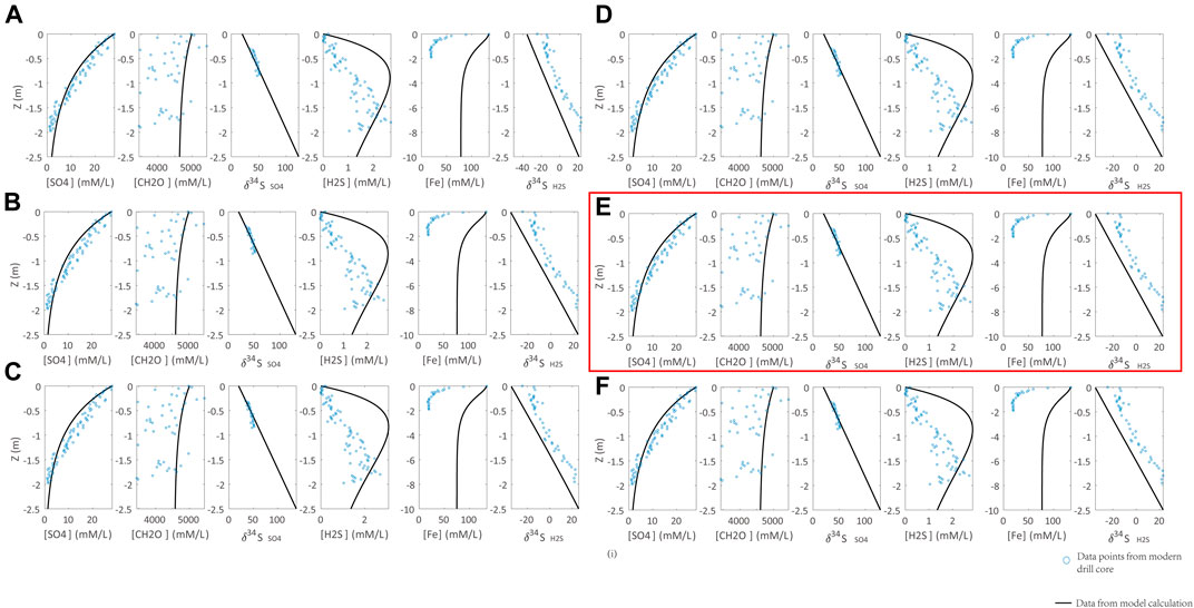
FIGURE 3. Calibration of the DSR reaction rate constant (R_DSR) with observations from modern marine sediments (Soutar and Crill, 1977; Raven et al., 2016). Parameters of calculations are R_py = 0.3 [(mM/L)*ka]⁻¹, Δ_DSR = 70‰. R_DSR is set to (A) 0.003, (B) 0.0035, (C) 0.004, (D) 0.0032, (E) 0.0033, (F) 0.0034 [(mM/L)*ka]⁻¹. Blue points are the modern marine sediment samples. The black lines represent the modeling results. R_DSR = 0.0033 [(mM/L)*ka]⁻¹ in (H) can simulate the sulfate profile of modern marine sediments (highlighted by red box).

In addition, the porewater profile of sulfur isotope composition of porewater sulfate (δ³⁴S_pw) is controlled by Δ_DSR, R_DSR, (Org0), and seawater sulfate concentration. It is proposed that Δ_DSR is 46‰ if sulfate concentration is greater than 0.2 mM (Habicht and Canfield, 1997; Habicht et al., 2002). Recent studies indicate that the isotopic difference between seawater sulfate and sediment pyrite can be up to 70‰ in the past 500 ky (Pasquier et al., 2017). Thus, we allow Δ_DSR varying between 46 and 70‰ (Figure 4). The modeling results indicate that Δ_DSR of 70‰ can best simulate the porewater δ³⁴S_pw profile of modern sediments. In fact, Δ_DSR of 70% is consistent with the cultural DSR experiments, which indicate a similar magnitude (up to 66‰) of Δ_DSR, if there is no sulfur disproportionation (Sim et al., 2011).

FIGURE 4

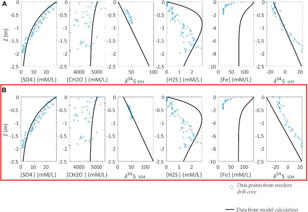
FIGURE 4. Calibration of the S isotope fractionation in DSR (Δ_DSR) with observations from modern marine sediments (Soutar and Crill, 1977; Raven et al., 2016). Parameters of calculations are R_py = 0.3 [(mM/L)*ka]⁻¹, R_DSR = 0.0033 [(mM/L)*ka]⁻¹. Δ_DSR is set to (A) 46‰, (B) 70‰. Blue points are the modern sediment samples. The black lines are the modeling results. Δ_DSR = 70‰ in (B) can simulate the sulfate profiles in modern marine sediments (highlighted by the red box).

Another key issue is the correlation between seawater/seafloor redox condition and pyrite formation reaction constant (R_py). R_py is a constant, but it is a variant in the model that is related to the seawater redox condition. Oxidation of H₂S is a complex process, involving the generation of different sulfur species of various valence states. Since we have ignored the formation of sulfur species with intermediate valence states and assumed sulfate as the only product of H₂S oxidation (Lang et al., 2020), recycling of H₂S-derived sulfate in DSR is excluded. In addition, H₂S oxidation could be further complicated by its possible connections with Fe/Mn oxidation, nitrate oxidation, and O₂ oxidation (Li et al., 2010). In order to simplify the simulation, we replace the seawater/seafloor redox condition with R_py. It is proposed that a larger R_py implies less H₂S oxidation, i.e., more reduced conditions. Furthermore, the oxidation of H₂S is simulated by the H₂S upward diffusion to seawater instead of the downward diffusion of oxidants into sediments. For these reasons, the profiles of H₂S concentration and isotope profiles can’t be well simulated in our model (Figure 5). In the simulation, we have R_py = 0.3 [(mM/L)*ka]⁻¹ as a cutoff value for euxinic bottom water, which is closest to the actual profiles with the seafloor oxygen fugacity (f_O2) < 10 uM (Figure 5). It should be noted that the linkage between R_py and seafloor f_O2 is not fixed due to the lack of modern observation.

FIGURE 5

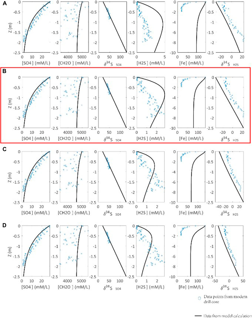
FIGURE 5. Calibration of the seawater redox condition and pyrite formation reaction constant (R_py) with an observation from modern marine sediments (Soutar and Crill, 1977; Raven et al., 2016). Parameters of calculations are Δ_DSR = 70‰, R_DSR = 0.0033 [(mM/L)*ka]⁻¹. R_py is set to (A) 0.1, (B) 0.3, (C) 0.5, (D) 0.7 [(mM/L)*ka]⁻¹. Blue points are data points of observation from the modern drill core. Concentration and S isotope composition profile of H₂S cannot be well simulated by our model, due to simplification of oxidation mechanism of H₂S. We choose R_py = 0.3 [(mM/L)*ka]⁻¹ in (B) to represent seawater redox condition of O₂ < 10 uM in modern drill core (highlighted by red box).

The Monte Carlo Simulation

Because the number of parameters is much larger than the number of equations, there are multiple solutions in quantifying the seawater sulfate concentration with pyrite sulfur isotope and pyrite contents. To reduce the uncertainties raised by loosely constrained parameters, here, we apply the Monte Carlo simulation. In this method, each parameter is allowed a range of variation (Table 2). All possible solutions are calculated based on each assemblage of parameters. If there are n parameters, each of which has m_i possible values (i ranges from 1 to n). There are ${\displaystyle \prod }_i^n{m}_i$ assemblages or outputs.

TABLE 2

TABLE 2. List of parameters used in the model.

To save the computation resource, we take the following assumptions. 1) Sedimentation rate of similar lithology in the same section is limited to a narrow range (0.05–0.15 m/ky for our samples). This assumption is generally consistent with the estimation of sedimentation rate based on the available biostratigraphic data. In detail, the Yurtus Formation with a total thickness of ∼60 m was deposited within 21 million years, including black shale of ∼30 m, dolomite of 3.3 m, and carbonate dominated interval of ∼27 m (Zhu et al., 2021). Considering the faster precipitation of carbonate rocks, it is estimated that the black shale was deposited between 10.5 and 21 million years. Assuming the compaction rate of 0.8, the sedimentation rate of muddy sediment (black shale) in the Yurtus Formation is between 0.075 and 0.15 m/ky. 2) Pyrite is the only major sink for reactive Fe and precipitates in sediment porewater. The second assumption allows the replacement of pyrite content by Fe_PY/Fe_HR ratio. In addition, this also implies (Fe0) equals to Fe_HR. For each sample, if Fe_PY/Fe_HR and δ³⁴S_py fall between the two nearby input points, the input points are included in the solution.

In addition, to limit the multiplicity of solution from multiple samples, we have the following assumptions. 1) The seawater sulfate concentration is invariant for samples from the same section (non-sulfidic seawater). This is likely the case given the residence time of seawater sulfate is longer than the duration of sample collections (the Geological Background section). 2) The seawater/seafloor redox condition was the same for all samples of the same lithology. For each set of seawater sulfate concentration and seawater/seafloor redox condition values, we calculate the frequency that the solution set of samples contains the seawater sulfate concentration range and the seawater redox condition range (Table 3). Because sulfate concentration is homogeneous in non-sulfidic seawater, the seawater sulfate concentration range with the frequency of 1 (indicating possible for all samples) is the plausible range of seawater sulfate concentration.

TABLE 3

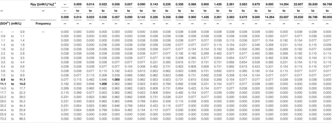
TABLE 3. Frequency map on seawater sulfate concentration and redox condition. Frequency = 1 (highlight by overstriking word) indicates possible seawater sulfate concentration 8.9–14.0 mM (highlight by overstriking word) for all samples.

Technically, we justified the two parameters, R_DSR and Δ_DSR, based on the simulations of porewater geochemical profiles of modern marine sediments. Furthermore, to eliminate uncertainties raised by other loosely constrained or unconstrained parameters, such as sedimentation rate and redox condition, we run the Monte Carlo simulation to calculate all possible outcomes. With certain constraints from geological observations and by assuming homogeneous seawater sulfate concentration, the seawater sulfate concentration of the early Cambrian ocean can be quantified by δ³⁴S_py and Fe speciation data. Below, we will calculate the early Cambrian seawater sulfate concentration by this methodology.

Quantifying the Early Cambrian Seawater Sulfate Concentration

The sulfate concentration should be homogeneous in non-sulfidic seawater because the ocean mixing time is four orders of magnitude shorter than the residence time of seawater sulfate (1000s of years vs. 10s million years). Even the seawater sulfate concentration was an order of magnitude lower (Loyd et al., 2012), a homogeneous seawater sulfate concentration in the non-sulfidic seawater is still valid in a million-year time scale. In contrast, because of active DSR in sulfidic seawater, the sulfate concentration in sulfidic seawater could be different from non-sulfidic seawater (Lyons, 1997). Thus, this model can only be applied to the non-sulfidic ocean.

It is noticed that some Yurtus samples have Fe_PY/Fe_HR ratios >0.8, suggesting the deposition under sulfidic conditions (Poulton and Raiswell, 2002; Raiswell et al., 2018). However, deposition under sulfidic conditions is inconsistent with abundant fossils from the Yurtus Formation, including typical early Cambrian Asteridium-Heliosphaeridium-Comasphaeridium acritarch assemblage, and tubular fossil Megathrix, as well as small shelly fossils including Shabaktiella multiformis, Parcaconus xinjiangensis, Eoyochelcionella aksuensis (Qian, 1999; Qian et al., 2001; Yao et al., 2005; Dong et al., 2009), the latter of which implies the seafloor might be habitable for animals. In fact, recent studies indicate that the terrestrial input of reactive Fe is strongly affected by the intensity of continental weathering (Wei et al., 2021), implying that the Fe_HR/Fe_T ratio is not only affected by the redox condition of seawater. Similarly, pyrite precipitation within sediment porewater is affected by many factors, and a high fraction (high Fe_PY/Fe_HR ratio) of syndepositional pyrite could be generated in non-sulfidic conditions (Lang et al., 2020). Deposition in a non-sulfidic water column is also consistent with abundant diagenetic euhedral pyrites from the Yurtus Formation. Therefore, we argue that the above simulations can be applied to the Yurtus samples.

To validate the calculated seawater sulfate concentration from the Tarim samples, we also choose samples from the Yangtze Block, South China. The early Cambrian successions in the Yangtze Block have been extensively studied, and several sections have both δ³⁴S_py and Fe speciation data reported, including the Xiaotan section (Och et al., 2016), Shatan and Songtao sections (Goldberg et al., 2007), Jinsha and Weng’an sections (Jin et al., 2016), Dingtai section (Xu et al., 2012), Yangjiaping section (Feng et al., 2014), and Longbizui section (Wang et al., 2012). As discussed above, this model can only simulate syndepositional pyrite formation in non-sulfidic seawater. Although there are many samples from the Yangtze Block that might have been deposited under non-sulfidic conditions, the sampling interval from the Yangtze Block should overlap with that of the Yurtus Formation in the Tarim Block. Thus, we choose data from the Songtao section for analysis (Goldberg et al., 2007).

In the simulation, we use Fe speciation data and δ³⁴S_py data from the Yurtus Formation in the X1 drill core in the Tarim Block and from the Niutitang Formation (∼529−515 Ma) (Jin et al., 2020; Na and Kiessling, 2015) in the Songtao section in the Yangtze Block. We also apply the calibrated R_DSR and Δ_DSR values (Figures 3,4). The early Cambrian δ³⁴S_SW is set to +30‰ (Fike et al., 2015). Although the validity of δ³⁴S_CAS has been challenged (Marenco et al., 2008; Peng et al., 2014), the assigned δ³⁴S_SW value is consistent with the δ³⁴S_CAS data from the Yurtus Formation (Figure 2). Other parameters are allowed a range of variation, which are listed in Table 1.

Based on the outputs of the simulation, the frequency map of both seawater sulfate concentration and redox condition for all samples can be created (Table 3). The seawater sulfate concentration is bracketed between 8.9 and 14.0 mM. These values are in agreement with a rough estimate of ∼10 mM based on the marine sulfur isotope mass balance calculation (Canfield and Farquhar, 2009), but at least 4 times higher than the calculation of ∼2 mM based on the stratigraphic variation of CAS sulfur isotope values (Loyd et al., 2012).

Our modeling result indicates that the seawater sulfate concentration was already high during the early Cambrian, equivalent to ∼30–50% of the present level of 28 mM. The seawater sulfate concentration is controlled by both terrestrial input of sulfate and burial in the ocean. Evaporate deposition (mainly gypsum) and pyrite precipitation and burial are the two major sinks of seawater sulfate (Fike et al., 2015). It is unclear how seawater sulfate concentration could increase to 30–50% of the present level. Neither is known about when the seawater sulfate concentration increased during the EdiacaranCambrian transition. We suggest that high seawater sulfate concentration during the early Cambrian might be favored due to the following reasons. First, the terrestrial sulfate input might have dramatically increased due to extensive evaporate dissolution during the formation of “Great Unconformity” (Peters and Gaines, 2012; Shields et al., 2019). Second, although the redox landscape in the early Cambrian ocean might be highly heterogeneous with the possible development of sulfidic wedge in continental margins (Jin et al., 2014; Jin et al., 2016; Li et al., 2018), the proportion of sulfidic seafloor might be smaller than that of early Neoproterozoic and Mesoproterozoic (Lyons et al., 2014). Limited seafloor euxinia also indicates less efficient pyrite burial, reducing the pyrite sink of the seawater sulfate. This argument is consistent with high Mo content in the lower Cambrian black shales (Sahoo et al., 2012; Reinhard et al., 2013; Sahoo et al., 2016).

Finally, our model provides a new approach to quantify the seawater sulfate concentration in paleoceans. In addition to justifying some key parameters based on the modern sediment observation, the Monte Carlo simulation could reduce the uncertainties raised by loosed constrained parameters. It should be noted that the assumption of the Monte Carlo simulation is invariant seawater sulfate concentration during the interval of simulation. Thus, high-resolution sampling from non-sulfidic deposits is required. If samples were collected from multiple sections, the chrono- and/or biostratigraphic framework is required to justify the coeval deposition.

Conclusion

In this study, we justified the key parameters (reaction rate constant of DSR and sulfur isotopic fractionation in DSR) of the syndepositional pyrite formation model. We also develop the Monte Carlo simulation approach to avoid uncertainties raised by loosely constrained parameters, such as sedimentation rate and the initial organic matter content in sediment. The new model allows the quantification of seawater sulfate concentration in deep time by using pyrite sulfur isotope and Fe speciation data. Based on the study of the lower Cambrian Yurtus Formation in the Tarim Block, combining with the data of the coeval Niutitang Formation in the Yangtze Block, the early Cambrian seawater sulfate concentration is bracketed between 8.9 and 14.0 mM, approaching to 30–50% of the present level. The relatively high seawater sulfate concentration might be attributed to enhanced terrestrial sulfate input in the context of “the Great Unconformity” and the reduced sulfidic seafloor in the second rise of atmospheric O₂ level. Our model provides a new approach to quantify the seawater sulfate concentration in paleoceans.

Data Availability Statement

The raw data supporting the conclusion of this article will be made available by the authors, without undue reservation.

Author Contributions

BS, TH and XL contributed to conception and design of the study. GZ, TL and KZ collected and analysed samples. TH, BS, XL, WT, and RW contributed to modeling and data analyzing. TH and BS wrote sections of the manuscript. All authors contributed to manuscript revision, read, and approved the submitted version.

Funding

This project was funded by the Scientific Research and Technology Development Project of China National Petroleum Corporation (CNPC) (Grant Nos: 2019B-04 and 2018A-0102).

Conflict of Interest

GZ and TL were employed by the company China National Petroleum Corporation.

The remaining authors declare that the research was conducted in the absence of any commercial or financial relationships that could be construed as a potential conflict of interest.

The handling Editor declared a past co-authorship/collaboration with the authors (TH, XL and BS).

Publisher’s Note

All claims expressed in this article are solely those of the authors and do not necessarily represent those of their affiliated organizations, or those of the publisher, the editors and the reviewers. Any product that may be evaluated in this article, or claim that may be made by its manufacturer, is not guaranteed or endorsed by the publisher.

Acknowledgments

We acknowledge generous funding from China National Petroleum Corporation. We would like to thank Li Chao from China University of Geosciences (Wuhan) for Fe-speciation and sulfur isotope measurements and Bian Lizeng from Nanjing University for discussion about the depositional age of the Yurtus Formation.

Supplementary Material

The Supplementary Material for this article can be found online at: https://www.frontiersin.org/articles/10.3389/feart.2021.767857/full#supplementary-material

References

Brocks, J. J., Jarrett, A. J. M., Sirantoine, E., Hallmann, C., Hoshino, Y., and Liyanage, T. (2017). The Rise of Algae in Cryogenian Oceans and the Emergence of Animals. Nature 548, 578–581. doi:10.1038/nature23457

PubMed Abstract | CrossRef Full Text | Google Scholar

Canfield, D. E., and Farquhar, J. (2009). Animal Evolution, Bioturbation, and the Sulfate Concentration of the Oceans. Proc. Natl. Acad. Sci. 106, 8123–8127. doi:10.1073/pnas.0902037106

PubMed Abstract | CrossRef Full Text | Google Scholar

Canfield, D. E., Poulton, S. W., and Narbonne, G. M. (2007). Late-Neoproterozoic Deep-Ocean Oxygenation and the Rise of Animal Life. Science 315, 92–95. doi:10.1126/science.1135013

PubMed Abstract | CrossRef Full Text | Google Scholar

Canfield, D. E. (2004). The Evolution of the Earth Surface Sulfur Reservoir. Am. J. Sci. 304, 839–861. doi:10.2475/ajs.304.10.839

CrossRef Full Text | Google Scholar

Canfield, D., and Thamdrup, B. (1994). The Production of 34S-Depleted Sulfide during Bacterial Disproportionation of Elemental Sulfur. Science 266, 1973–1975. doi:10.1126/science.11540246

PubMed Abstract | CrossRef Full Text | Google Scholar

Ding, W., Dong, L., Sun, Y., Ma, H., Xu, Y., Yang, R., et al. (2019). Early Animal Evolution and Highly Oxygenated Seafloor Niches Hosted by Microbial Mats. Sci. Rep. 9, 13628. doi:10.1038/s41598-019-49993-2

PubMed Abstract | CrossRef Full Text | Google Scholar

Dong, L., Xiao, S., Shen, B., Zhou, C., Li, G., and Yao, J. (2009). Basal Cambrian Microfossils from the Yangtze Gorges Area (South China) and the Aksu Area (Tarim Block, Northwestern China). J. Paleontol. 83, 30–44. doi:10.1666/07-147r.1

CrossRef Full Text | Google Scholar

Du, J., and Pan, W. (2016). Accumulation Conditions and Play Targets of Oil and Gas in the Cambrian Subsalt dolomite,Tarim Basin, NW China. Pet. Exploration Dev. 43, 327–339. doi:10.1016/s1876-3804(16)30043-x

CrossRef Full Text | Google Scholar

Feng, L., Li, C., Huang, J., Chang, H., and Chu, X. (2014). A Sulfate Control on marine Mid-depth Euxinia on the Early Cambrian (Ca. 529-521Ma) Yangtze Platform, South China. Precambrian Res. 246, 123–133. doi:10.1016/j.precamres.2014.03.002

CrossRef Full Text | Google Scholar

Fike, D. A., Bradley, A. S., and Rose, C. V. (2015). Rethinking the Ancient Sulfur Cycle. Annu. Rev. Earth Planet. Sci. 43, 593–622. doi:10.1146/annurev-earth-060313-054802

CrossRef Full Text | Google Scholar

Fike, D. A., Grotzinger, J. P., Pratt, L. M., and Summons, R. E. (2006). Oxidation of the Ediacaran Ocean. Nature 444, 744–747. doi:10.1038/nature05345

PubMed Abstract | CrossRef Full Text | Google Scholar

Glaessner, M. F. (1984). The Dawn of Animal Life: A Biohistorical Study. Cambridge, UK: Cambridge Univ. Press.

Google Scholar

Goldberg, T., Strauss, H., Guo, Q., and Liu, C. (2007). Reconstructing marine Redox Conditions for the Early Cambrian Yangtze Platform: Evidence from Biogenic sulphur and Organic Carbon Isotopes. Palaeogeogr. Palaeoclimatol. Palaeoecol. 254, 175–193. doi:10.1016/j.palaeo.2007.03.015

CrossRef Full Text | Google Scholar

Gradstein, F. M. (2012). The Geological Time Scale 2012. Amsterdam, Netherlands ; Boston, MA: Elsevier.

Google Scholar

Grotzinger, J. P., Fike, D. A., and Fischer, W. W. (2011). Enigmatic Origin of the Largest-Known Carbon Isotope Excursion in Earth's History. Nat. Geosci 4, 285–292. doi:10.1038/ngeo1138

CrossRef Full Text | Google Scholar

Habicht, K. S., Canfield, D. E., and Rethmeier, J. (1998). Sulfur Isotope Fractionation during Bacterial Reduction and Disproportionation of Thiosulfate and Sulfite. Geochimica et Cosmochimica Acta 62, 2585–2595. doi:10.1016/s0016-7037(98)00167-7

CrossRef Full Text | Google Scholar

Habicht, K. S., and Canfield, D. E. (1997). Sulfur Isotope Fractionation during Bacterial Sulfate Reduction in Organic-Rich Sediments. Geochimica et Cosmochimica Acta 61, 5351–5361. doi:10.1016/s0016-7037(97)00311-6

PubMed Abstract | CrossRef Full Text | Google Scholar

Habicht, K. S., Gade, M., Thamdrup, B., Berg, P., and Canfield, D. E. (2002). Calibration of Sulfate Levels in the Archean Ocean. Science 298, 2372–2374. doi:10.1126/science.1078265

PubMed Abstract | CrossRef Full Text | Google Scholar

He, J., Qing, H., and Xu, B. (2018). The Unconformity-Related Palaeokarst in the Uppermost Ediacaran Carbonate Rocks in the Northwestern Tarim Block, NW China: Implication for Sedimentary Evolution During the Ediacaran-Cambrian Transition. Int. Geol. Rev. 61, 839–852. doi:10.1080/00206814.2018.1474498

CrossRef Full Text | Google Scholar

He, J., Wu, G., Xu, B., Qu, T., Li, H., and Cao, Y. (2010). Characteristics and Petroleum Exploration Significance of Unconformity between Sinian and Cambrian in Tarim Basin. Dizhi kexue 45, 698–706. doi:10.3969/j.issn.0563-5020.2010.03.006

CrossRef Full Text | Google Scholar

Jin, C., Li, C., Algeo, T. J., Planavsky, N. J., Cui, H., Yang, X., et al. (2016). A Highly Redox-Heterogeneous Ocean in South China during the Early Cambrian (∼529-514 Ma): Implications for Biota-Environment Co-evolution. Earth Planet. Sci. Lett. 441, 38–51. doi:10.1016/j.epsl.2016.02.019

CrossRef Full Text | Google Scholar

Jin, C., Li, C., Algeo, T. J., Wu, S., Cheng, M., Zhang, Z., et al. (2020). Controls on Organic Matter Accumulation on the Early-Cambrian Western Yangtze Platform, South China. Mar. Pet. Geology. 111, 75–87. doi:10.1016/j.marpetgeo.2019.08.005

CrossRef Full Text | Google Scholar

Jin, C., Li, C., Peng, X., Cui, H., Shi, W., Zhang, Z., et al. (2014). Spatiotemporal Variability of Ocean Chemistry in the Early Cambrian, South China. Sci. China Earth Sci. 57, 579–591. doi:10.1007/s11430-013-4779-y

CrossRef Full Text | Google Scholar

Kah, L. C., Lyons, T. W., and Frank, T. D. (2004). Low marine Sulphate and Protracted Oxygenation of the Proterozoic Biosphere. Nature 431, 834–838. doi:10.1038/nature02974

PubMed Abstract | CrossRef Full Text | Google Scholar

Kaufman, A. J., Corsetti, F. A., and Varni, M. A. (2007). The Effect of Rising Atmospheric Oxygen on Carbon and Sulfur Isotope Anomalies in the Neoproterozoic Johnnie Formation, Death Valley, USA. Chem. Geology. 237, 47–63. doi:10.1016/j.chemgeo.2006.06.023

CrossRef Full Text | Google Scholar

Lang, X., Tang, W., Ma, H., and Shen, B. (2020). Local Environmental Variation Obscures the Interpretation of Pyrite Sulfur Isotope Records. Earth Planet. Sci. Lett. 533, 116056. doi:10.1016/j.epsl.2019.116056

CrossRef Full Text | Google Scholar

Li, C., Cheng, M., Zhu, M., and Lyons, T. W. (2018). Heterogeneous and Dynamic Marine Shelf Oxygenation and Coupled Early Animal Evolution. Emerging Top. Life Sci. 2, 279–288. doi:10.1042/etls20170157

CrossRef Full Text | Google Scholar

Li, C., Love, G. D., Lyons, T. W., Fike, D. A., Sessions, A. L., and Chu, X. (2010). A Stratified Redox Model for the Ediacaran Ocean. Science 328, 80–83. doi:10.1126/science.1182369

PubMed Abstract | CrossRef Full Text | Google Scholar

Li, Z. X., Bogdanova, S. V., Collins, A. S., Davidson, A., De Waele, B., Ernst, R. E., et al. (2008). Assembly, Configuration, and Break-Up History of Rodinia: A Synthesis. Precambrian Res. 160, 179–210. doi:10.1016/j.precamres.2007.04.021

CrossRef Full Text | Google Scholar

Liu, P., Xiao, S., Yin, C., Chen, S., Zhou, C., and Li, M. (2014). Ediacaran Acanthomorphic Acritarchs and Other Microfossils from Chert Nodules of the Upper Doushantuo Formation in the Yangtze Gorges Area, South China. J. Paleontol. 88, 1–139. doi:10.1666/13-009

CrossRef Full Text | Google Scholar

Loyd, S. J., Marenco, P. J., Hagadorn, J. W., Lyons, T. W., Kaufman, A. J., Sour-Tovar, F., et al. (2012). Sustained Low marine Sulfate Concentrations from the Neoproterozoic to the Cambrian: Insights from Carbonates of Northwestern Mexico and Eastern California. Earth Planet. Sci. Lett. 339-340, 79–94. doi:10.1016/j.epsl.2012.05.032

CrossRef Full Text | Google Scholar

Lyons, T. W., Reinhard, C. T., and Planavsky, N. J. (2014). The Rise of Oxygen in Earth's Early Ocean and Atmosphere. Nature 506, 307–315. doi:10.1038/nature13068

PubMed Abstract | CrossRef Full Text | Google Scholar

Lyons, T. W. (1997). Sulfur Isotopic Trends and Pathways of Iron Sulfide Formation in Upper Holocene Sediments of the Anoxic Black Sea. Geochimica et Cosmochimica Acta 61, 3367–3382. doi:10.1016/s0016-7037(97)00174-9

CrossRef Full Text | Google Scholar

Marenco, P. J., Corsetti, F. A., Hammond, D. E., Kaufman, A. J., and Bottjer, D. J. (2008). Oxidation of Pyrite during Extraction of Carbonate Associated Sulfate. Chem. Geology. 247, 124–132. doi:10.1016/j.chemgeo.2007.10.006

CrossRef Full Text | Google Scholar

McFadden, K. A., Huang, J., Chu, X., Jiang, G., Kaufman, A. J., Zhou, C., et al. (2008). Pulsed Oxidation and Biological Evolution in the Ediacaran Doushantuo Formation. Proc. Natl. Acad. Sci. 105, 3197–3202. doi:10.1073/pnas.0708336105

PubMed Abstract | CrossRef Full Text | Google Scholar

Na, L., and Kiessling, W. (2015). Diversity Partitioning during the Cambrian Radiation. Proc. Natl. Acad. Sci. USA 112, 4702–4706. doi:10.1073/pnas.1424985112

PubMed Abstract | CrossRef Full Text | Google Scholar

Narbonne, G. M. (2005). The Ediacara Biota: Neoproterozoic Origin of Animals and Their Ecosystems. Annu. Rev. Earth Planet. Sci. 33, 421–442. doi:10.1146/annurev.earth.33.092203.122519

CrossRef Full Text | Google Scholar

Och, L. M., Cremonese, L., Shields-Zhou, G. A., Poulton, S. W., Struck, U., Ling, H., et al. (2016). Palaeoceanographic Controls on Spatial Redox Distribution over the Yangtze Platform during the Ediacaran-Cambrian Transition. Sedimentology 63, 378–410. doi:10.1111/sed.12220

CrossRef Full Text | Google Scholar

Pasquier, V., Sansjofre, P., Rabineau, M., Revillon, S., Houghton, J., and Fike, D. A. (2017). Pyrite Sulfur Isotopes Reveal Glacial−interglacial Environmental Changes. Proc. Natl. Acad. Sci. USA 114, 5941–5945. doi:10.1073/pnas.1618245114

PubMed Abstract | CrossRef Full Text | Google Scholar

Peng, Y., Bao, H., Pratt, L. M., Kaufman, A. J., Jiang, G., Boyd, D., et al. (2014). Widespread Contamination of Carbonate-Associated Sulfate by Present-Day Secondary Atmospheric Sulfate: Evidence from Triple Oxygen Isotopes. Geology 42, 815–818. doi:10.1130/g35852.1

CrossRef Full Text | Google Scholar

Peters, S. E., and Gaines, R. R. (2012). Formation of the 'Great Unconformity' as a Trigger for the Cambrian Explosion. Nature 484, 363–366. doi:10.1038/nature10969

PubMed Abstract | CrossRef Full Text | Google Scholar

Poulton, S. W., and Raiswell, R. (2002). The Low-Temperature Geochemical Cycle of Iron: From continental Fluxes to marine Sediment Deposition. Am. J. Sci. 302, 774–805. doi:10.2475/ajs.302.9.774

CrossRef Full Text | Google Scholar

Qian, M., Yuan, X., Xiao, S., Li, J., and Wang, Y. (2000). Neoproterozoic Glaciations and Their Triggers in the Yangtze Platform. Jiangsu Geology. 24, 135–139. doi:10.1080/00206814.2018.1474498

CrossRef Full Text | Google Scholar

Qian, Y., Li, G., and Zhu, M. (2001). The Meishucunian Stage and its Small Shelly Fossil Sequence in China. Acta Palaeontologica Sinica 40 (Suppl. ment), 54–62.

Google Scholar

Qian, Y. (1999). Taxonomy and Biostratigraphy of Small Shelly Fossils in China. Beijing: Science Press.

Google Scholar

Raiswell, R., Hardisty, D. S., Lyons, T. W., Canfield, D. E., Owens, J. D., Planavsky, N. J., et al. (2018). The Iron Paleoredox Proxies: A Guide to the Pitfalls, Problems and Proper Practice. Am. J. Sci. 318, 491–526. doi:10.2475/05.2018.03

CrossRef Full Text | Google Scholar

Raven, M. R., Sessions, A. L., Fischer, W. W., and Adkins, J. F. (2016). Sedimentary Pyrite δ34S Differs from Porewater Sulfide in Santa Barbara Basin: Proposed Role of Organic Sulfur. Geochimica et Cosmochimica Acta 186, 120–134. doi:10.1016/j.gca.2016.04.037

CrossRef Full Text | Google Scholar

Reinhard, C. T., Planavsky, N. J., Robbins, L. J., Partin, C. A., Gill, B. C., Lalonde, S. V., et al. (2013). Proterozoic Ocean Redox and Biogeochemical Stasis. Proc. Natl. Acad. Sci. 110, 5357–5362. doi:10.1073/pnas.1208622110

PubMed Abstract | CrossRef Full Text | Google Scholar

Sahoo, S. K., Planavsky, N. J., Jiang, G., Kendall, B., Owens, J. D., Wang, X., et al. (2016). Oceanic Oxygenation Events in the Anoxic Ediacaran Ocean. Geobiology 14, 457–468. doi:10.1111/gbi.12182

PubMed Abstract | CrossRef Full Text | Google Scholar

Sahoo, S. K., Planavsky, N. J., Kendall, B., Wang, X., Shi, X., Scott, C., et al. (2012). Ocean Oxygenation in the Wake of the Marinoan Glaciation. Nature 489, 546–549. doi:10.1038/nature11445

PubMed Abstract | CrossRef Full Text | Google Scholar

Shields, G. A., Mills, B. J. W., Zhu, M., Raub, T. D., Daines, S. J., and Lenton, T. M. (2019). Unique Neoproterozoic Carbon Isotope Excursions Sustained by Coupled Evaporite Dissolution and Pyrite Burial. Nat. Geosci. 12, 823–827. doi:10.1038/s41561-019-0434-3

CrossRef Full Text | Google Scholar

Shields-Zhou, G., and Och, L. (2011). The Case for a Neoproterozoic Oxygenation Event: Geochemical Evidence and Biological Consequences. Gsat 21, 4–11. doi:10.1130/gsatg102a.1

CrossRef Full Text | Google Scholar

Sim, M. S., Bosak, T., and Ono, S. (2011). Large Sulfur Isotope Fractionation Does Not Require Disproportionation. Science 333, 74–77. doi:10.1126/science.1205103

PubMed Abstract | CrossRef Full Text | Google Scholar

Soutar, A., and Crill, P. A. (1977). Sedimentation and Climatic Patterns in the Santa Barbara Basin during the 19th and 20th Centuries. Geol. Soc. America Bull. 88, 1161–1172. doi:10.1130/0016-7606(1977)88<1161:sacpit>2.0.co;2

CrossRef Full Text | Google Scholar

Thompson, C. K., and Kah, L. C. (2012). Sulfur Isotope Evidence for Widespread Euxinia and a Fluctuating Oxycline in Early to Middle Ordovician Greenhouse Oceans. Palaeogeogr. Palaeoclimatol. Palaeoecol. 313-314, 189–214. doi:10.1016/j.palaeo.2011.10.020

CrossRef Full Text | Google Scholar

Wang, J., Chen, D., Yan, D., Wei, H., and Xiang, L. (2012). Evolution from an Anoxic to Oxic Deep Ocean during the Ediacaran-Cambrian Transition and Implications for Bioradiation. Chem. Geology. 306-307, 129–138. doi:10.1016/j.chemgeo.2012.03.005

CrossRef Full Text | Google Scholar

Wei, G.-Y., Chen, T., Poulton, S. W., Lin, Y.-B., He, T., Shi, X., et al. (2021). A Chemical Weathering Control on the Delivery of Particulate Iron to the continental Shelf. Geochimica et Cosmochimica Acta 308, 204–216. doi:10.1016/j.gca.2021.05.058

CrossRef Full Text | Google Scholar

Xu, L., Lehmann, B., Mao, J., Nägler, T. F., Neubert, N., Böttcher, M. E., et al. (2012). Mo Isotope and Trace Element Patterns of Lower Cambrian Black Shales in South China: Multi-Proxy Constraints on the Paleoenvironment. Chem. Geology. 318-319, 45–59. doi:10.1016/j.chemgeo.2012.05.016

CrossRef Full Text | Google Scholar

Yao, J., Xiao, S., Yin, L., Li, G., and Yuan, X. (2005). Basal Cambrian Microfossils from the Yurtus and Xishanblaq Formations (Tarim, North-west China): Systematic Revision and Biostratigraphic Correlation of Micrhystridium-like Acritarchs. Palaeontology 48, 687–708. doi:10.1111/j.1475-4983.2005.00484.x

CrossRef Full Text | Google Scholar

Yin, L., Zhu, M., Knoll, A. H., Yuan, X., Zhang, J., and Hu, J. (2007). Doushantuo Embryos Preserved inside Diapause Egg Cysts. Nature 446, 661–663. doi:10.1038/nature05682

PubMed Abstract | CrossRef Full Text | Google Scholar

Yuan, X., Chen, Z., Xiao, S., Zhou, C., and Hua, H. (2011). An Early Ediacaran Assemblage of Macroscopic and Morphologically Differentiated Eukaryotes. Nature 470, 390–393. doi:10.1038/nature09810

PubMed Abstract | CrossRef Full Text | Google Scholar

Zhang, F., Xiao, S., Kendall, B., Romaniello, S. J., Cui, H., Meyer, M., et al. (2018). Extensive marine Anoxia during the Terminal Ediacaran Period. Sci. Adv. 4, eaan8983. doi:10.1126/sciadv.aan8983

PubMed Abstract | CrossRef Full Text | Google Scholar

Zhang, Y. (1989). Multicellular Thallophytes with Differentiated Tissues from Late Proterozoic Phosphate Rocks of South China. Lethaia 22, 113–132. doi:10.1111/j.1502-3931.1989.tb01164.x

CrossRef Full Text | Google Scholar

Zhu, G., Chen, F., Wang, M., Zhang, Z., Ren, R., and Wu, L. (2018). Discovery of the Lower Cambrian High-Quality Source Rocks and Deep Oil and Gas Exploration Potential in the Tarim Basin, China. Bulletin 102, 2123–2151. doi:10.1306/03141817183

CrossRef Full Text | Google Scholar

Zhu, G., Li, T., Zhao, K., Li, C., Cheng, M., Chen, W., et al. (2021). Mo Isotope Records from Lower Cambrian Black Shales, Northwestern Tarim Basin (China): Implications for the Early Cambrian Ocean. Geological Society of America bulletin. doi:10.1130/B35726.1

CrossRef Full Text | Google Scholar