High-Resolution Imaging: An Approach by Compensating Absorption and Dispersion in Prestack Time Migration With Effective Q Estimation and Fresnel Zone Identification Based on Deep Learning

We have developed a migration scheme that can compensate absorption and dispersion with effective $Q$ estimation and Fresnel zone identification based on deep learning. We use the U-Net neural network technology in deep learning to automatically identify Fresnel zones from compensated migrated dip-angle gathers and obtain the optimal aperture for migration, avoiding the tedious task of manually modifying the boundaries of Fresnel zones. Instead of the interval $Q$ factor, we used an effective $Q$ parameter to compensate absorption and dispersion. The effective $Q$ is estimated using VSP well data and surface seismic velocity data. The proposed scheme can be incorporated into conventional seismic data processing workflow. A field data set was employed to validate the proposed scheme. Higher resolution imaging results with low noise levels are obtained.

1 Introduction

The dissipation of seismic energy is caused by the anelasticity of the subsurface medium, which will decrease the amplitude and modify the phase. In this dissipative medium, as the propagation distance of the seismic wave increases, the attenuation of the seismic wave becomes more serious. Therefore, seismic waves in deep and ultra-deep stratums face the problem of lower resolution due to dissipation. It is crucial to find an appropriate method to eliminate the absorption and dispersion effects of seismic waves for higher resolution. We commonly use the quality factor $Q$-related methods to compensate absorption and dispersion in seismic data processing, and most of them can be divided into two categories: one is the inverse $Q$ filtering (Hargreaves and Calvert, 1991; Wang, 2002; Ferber, 2005; Cavalca et al., 2011; Chen et al., 2014; Zhang et al., 2014; Dai et al., 2018; Shi et al., 2019; Sangwan and Kumar, 2021), and the other is the anelastic prestack migration based on the viscoacoustic wave equation (Zhang and Wapenaar, 2002; Xie et al., 2009; Zhang et al., 2013; Guo et al., 2016; Wang et al., 2018; Zhang et al., 2021). In the first category, inverse $Q$ filtering is based on the theory of 1-D wave backpropagation and cannot calculate the seismic wave propagation path accurately. In the second category, anelastic prestack depth migration (PSDM) utilizes the viscoacoustic wave equation to simulate wave propagation with dissipation in the wavefield extrapolation, which is a more accurate and consistent way; however, the calculation load is huge, and the interval $Q$ model is difficult to obtain. Because of the effectiveness of prestack time migration (PSTM) in imaging complex structures without strong velocity variations, various $Q$-compensated methods based on the PSTM structure have been developed (Zhang et al., 2013; Zhang et al., 2016; Wu et,al., 2019). These methods employ effective $Q$ parameters, rather than the interval $Q$ model used in the depth migration approach, and the estimation of an effective $Q$ model is easier to achieve than that of an interval $Q$ model.

An optimal migration aperture can improve the signal-to-noise ratio (S/N) of imaging results. Schleicher et al. (1997) pointed out that the Fresnel zone is an optimal migration aperture. The signal outside the Fresnel zone does not contribute to imaging but brings noise and artifacts, which reduces the quality of the imaging results (Chen 2004; Marfurt 2006; Klokov and Fomel 2012a; Yu et al., 2013). However, the low S/N of field data and underground complex structures make an accurate Fresnel zone estimation challenging. In recent years, some articles have realized the estimation of Fresnel zones in a simple domain, by constructing a migrated dip-angle gather in the time or depth domains (Zhang et al., 2016; Li et al., 2018; Cheng et al., 2020). Zhang et al. (2016) has applied conventional PSTM to generate migrated dip-angle gathers for Fresnel zone estimation during deabsorption of the PSTM process. Cheng et al. (2020) used a modified VGGNet (A convolutional neural network was developed by the University of Oxford’s Visual Geometry Group and Google DeepMind in 2014) to extract Fresnel zones from migrated dip-angle gathers, which is a useful attempt at deep learning for Fresnel zone estimation. However, these Fresnel zone estimation methods are all suitable for dip-angle gathers generated by conventional migration methods, and little research has been carried out on that using compensated dip-angle gathers with a high resolution generated by compensated migration methods.

The quality factor $Q$ is closely related to the rock properties of the formation, water saturation, seismic wave amplitude and frequency, and other factors; therefore, calculating the $Q$ value accurately is very difficult. To meet the demand for $Q$ in seismic data processing, many methods have been developed to estimate $Q$. The $Q$ estimation method was initially proposed using a vertical seismic profile (VSP) (Tonn, 1991) and crosswell data (Neep et al., 1996). These methods can obtain a small amount of $Q$ values because VSP and cross-well data are not always available in the field, and we prefer to estimate the $Q$ value from surface reflection seismic data. A variety of methods have been proposed to estimate the $Q$ value from surface seismic data, and most of them can be divided into two categories: one is the wavelet information–based method (Quan and Harris, 1997; Dasgupta and Clark, 1998; Zhang et al., 2013; Bettinelli Pet al., 2014), which is employed in the time or frequency domain (e.g., the frequency shift method and spectral-ratio method) and demonstrates good performance for estimation of the $Q$ value, whereas often suffers from noise and wavelet interferences, and the other one is the tomography inversion–based method (Brzostowski and McMechan, 1992; Shen et al., 2018). In the first category, Zhang et al. (2013) estimated the $Q$ value using surface seismic data by constant $Q$ migration scanning; however, the implementation complexity of this method limits its broader application. In the second category, the widely used ray-based tomography can estimate the Q value for the dominant frequency with expensive calculation cost and local instability (Cavalca et al., 2011; Shen and Zhu, 2015; Dutta and Schuster, 2016). Full-waveform inversion (FWI) is another popular inversion approach using waveform rather than travel-time, but it requires an accurate initial model and burdens a huge computational expense (Kamei and Pratt, 2008).

This article takes the estimations of the optimal aperture and effective $Q$ model as the research focus in the compensated PSTM, which is arranged as follows: first, we introduce a modified PSTM scheme with compensation based on the effective $Q$; second, we propose a Fresnel zone identification scheme based on compensated migrated dip-angle gathers using deep learning; third, we present an estimation approach of the effective $Q$ model for the compensated PSTM. Finally, we demonstrate our scheme with a field data set.

2 PSTM With Compensation Based on Effective Q

By following Zhang et al. (2013), a modified PSTM with compensation based on the effective Q model is expressed as

$I_Q\left(x,T\right)={\displaystyle \sum _{p=1}^n\mathrm{\Omega }\left(x,T_S,T_0\right)}\frac{{\tau }_s}{{\tau }_g}{\displaystyle \int f_p\left(\omega \right)\sqrt{\omega }\exp \left(-\frac{i\mathrm{\pi }}{4}\right)\exp \left[\mathrm{i}\omega \left({\tau }_s+{\tau }_g\right)\left(1-\frac{1}{\mathrm{\pi }{Q}_{eff}}\ln \frac{\omega }{{\omega }_0}\right)\right]}\exp \left[\frac{\omega \left({\tau }_s+{\tau }_g\right)}{2Q_{eff}}\right]\mathrm{d}\mathit{\omega },(1)$

where $f_p\left(\omega \right)$ is the Fourier transform of the p^th prestack trace, ${\tau }_s$ and ${\tau }_g$ represent the travel times from the shot and receiver to the imaging point, respectively, $T_0$ is the two-way vertical travel time, $\mathrm{\Omega }\left(x,T_S,T_0\right)$ represents the whole migration aperture, $T_s$ represents the starting travel time of the migration aperture, and $Q_{eff}$ is the effective $Q$ parameter. Eq. 1 denotes a compensated migration impulse response of a seismic trace. Summation of the impulse responses of all seismic traces yields a compensated migration result. The two $Q_{\text{eff}}$-related terms in Eq. 1 are the frequency-dependent dispersion and amplitude attenuation correction terms, respectively, which are different from the conventional PSTM. In Eq. 1, the size of the migration aperture has an important influence on the signal-to-noise ratio of the imaging result, and the accuracy of effective $Q$ determines the quality of the compensation result. In view of these two aspects, this article proposes a method of using deep learning to pick up the optimal aperture and a method of quickly obtaining the effective $Q$ model using VSP data and seismic velocity data. These two methods, together with the modified PSTM with compensation, form a seismic data imaging workflow that is specifically used for high-resolution imaging of prestack seismic data.

3 Identification of Fresnel Zones Using Deep Learning

Three separate sections are considered to introduce the theory of deep learning–based automated Fresnel zone extraction. The first section makes a review of migrated dip-angle gathers.

The second section introduces the architecture of the deep neural network adopted, including the design of U-Net input and output patterns and different types of layers in the network. The final section gives the loss function and training details in seeking optimal weights and biases of the network.

3.1 Review of Migrated Dip-Angle Gathers

Summing the migrated traces within Fresnel zones can produce a high S/N imaging profile. The migrated dip-angle gather supplies a simple domain that makes a visual pickup of Fresnel zones possible, which are constructed by sorting and summing the migrated results in the time or depth domains according to the dip angle (Zhang et al., 2016; Cheng et al., 2020). Different from the conventional migrated dip-angle gather, the compensated migrated dip-angle gather has the characteristics of high resolution and thin events. Therefore, the label data and training parameters of the trained network for conventional migrated dip-angle gathers must be relabeled and trained respectively when the neural network is applied to identify Fresnel zones using compensated migrated dip-angle gathers. In the next section, we will discuss how to use compensated dip-angle gathers to determine Fresnel zones of 2D seismic data. Figure 1 shows the geometrical relationship about the dip angle (Zhang et al., 2016). The angle can be expressed as follows:

$\tan \theta =\left[\left(x_s-x\right){\tau }_g+\left(x_g-x\right){\tau }_s\right]/\left[T{V}_{rms}\left({\tau }_s+{\tau }_g\right)\right],(2)$

where $\theta$ denotes the dip-angle related to travel time at the imaging point I; $V_{rms}$ is the root mean-square velocity at the imaging point; ${\tau }_s$ and ${\tau }_g$ represent the travel times from the shot ($x_s$) and receiver ($x_g$) to the imaging point I, respectively; and T represents the one-way vertical travel time. We obtained a 1D dip-angle gather by summing the migrated traces with dip angles ($\theta$) over the 2D imaging result. This process can be expressed as

$I\left(x,T,\theta \right)={\displaystyle \sum _{i=1}^{n}N\frac{{\tau }_s^2}{{\tau }_g^2}\stackrel{\sim }{f_i}\left({\tau }_s+{\tau }_g,x_s,x_g\right)}{\lambda }_i\left({\tau }_s+{\tau }_g,Q\right),(3)$

where n denotes the number of seismic traces, $\stackrel{\sim }{f_i}$ denotes a half-derivative of the i^th prestack seismic trace, and ${\lambda }_i$ is the corresponding compensation factor.

FIGURE 1

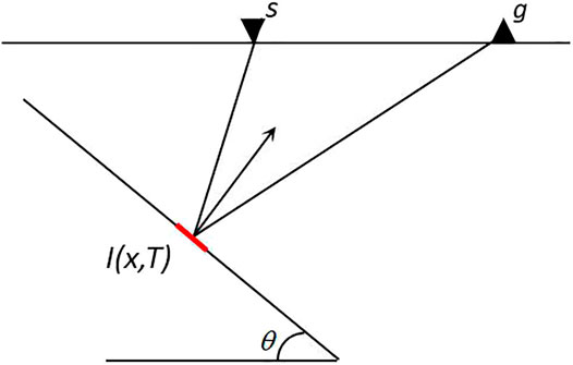
FIGURE 1. Illustration of the generation of a dip-angle gather. Points s and g denote the shot and receiver, respectively, and point I is the imaging point. $\theta$ represents the travel time–related dip-angle at the imaging point I.

The dip-angle gather shows a curved reflected event (Klokov and Fomel 2012b), and its vertex is the stationary-phase point (Cheng et al., 2020). The Fresnel zone is within half a wavelength near the stationary-phase point. Since the Fresnel zone is easy to identify in the dip-angle gather, we can pick it up through the dip-angle gather and obtain a high S/N migrated result by summing the Fresnel zones, but in practice, estimating Fresnel zones through dip-angle gathers will become challenging because dip-angle gathers will become correspondingly more complicated due to the low S/N of field data and underground complex structures, especially for imaging results with compensating absorption and dispersion since their dip-angle gathers differ in S/N and resolution from those generated by conventional migration, which add additional complexity. Many manual modifications to the Fresnel zone boundaries are required, which is a time-consuming and difficult task.

3.2 U-Net Architecture

Deep learning can think and process data just like the human brain, showing its superior capability in many fields in recent years (LeCun et al., 2015). It has multi-layer nonlinear activation function, which can discover hidden features in complex high-dimensional data by simulating signal transformation. Convolutional neural networks (CNNs) are currently the most successful and extensive application in deep learning, which connect input and output through multi-layer convolution. U-Net, a special type of CNN, was originally an auto-encoder–decoder network designed for medical image segmentation (Ronneberger, et al., 2015; A. Sevastopolsky, 2017; Wu et al., 2019; Zhang et al., 2021). We use U-Net to identify the left and right boundaries in the dip-angle gathers as the boundaries of Fresnel zones because one important reason is that U-Net can deliver a satisfactory performance even if the size of the training set is not very large. As shown in Figure 2, the main structure of the network includes two parts, down (encoder) and up (decoder), presenting a symmetrical form. Different levels of networks have different functions. The shallow layer is employed to solve the pixel positioning problem, while the deep layer is used to classify pixels. In the contraction path on the left, each step consists of two 3 × 3 convolution layers, followed by a rectified linear unit (ReLU) (Nair and Hinton, 2010; Krizhevsky et al., 2012) and a 2 × 2 max-pooling operation with stride 2 for downsampling. Symmetrically, each step on the right expansive path consists of a 2 × 2 upsampling operation with the same stride and two convolutional layers to halve feature channels. The sigmoid activation function is applied to the last channel feature vectors to produce a probability map of the output with the same size as the input. The skip connection is used in each upsampling operation, instead of directly monitoring and loss back-transmission on high-level semantic features, to integrate more low-level features into the finally recovered feature map. After building the network, we feed small volumes of seismic images generated by PSTM with compensation, together with corresponding labels. Each data volume contains 128 2D images with a size of 128 × 128. In order to avoid the odd-sized feature map encountered by the pooling layer, the same-padding convolution process was adopted in each step of the network.

FIGURE 2

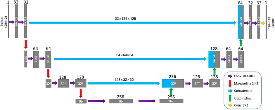
FIGURE 2. Simplified U-Net architecture. The black number describes the number of channels in feature maps. The purple arrow represents convolution-ReLU operation. The red arrow indicates the max-pooling operation which downsamples feature maps while the green arrow means the upsampling process. The blue arrow is the shortcut concatenating feature maps from shallow to deep layers.

3.3 Loss Function and Training

Network training uses a loss function to represent the difference between the true Fresnel zones and the predictions. The update of the parameters in the network is realized via the loss backpropagation (Rumelhart et al., 1986; Hecht-Nielsen, 1989), which is commonly used in the gradient descent optimization algorithm to iteratively adjust weights and biases of the neurons by calculating the gradient of the loss function. We consider the Fresnel zone identification problem as a binary segmentation problem; in other words, the output of the network is a probability distribution of 0–1, and the binary cross-entropy loss function is generally adopted:

$\mathrm{L}\mathrm{o}\mathrm{s}\mathrm{s}=-{\displaystyle \sum _{i=1}^n\left(b_i\times \ln a_i+\left(1-b_i\right)\times \ln \left(1-a_i\right)\right)},(4)$

where n is the number of pixels, $b_i$ denotes the true binary labels (0 or 1), and $a_i$ is the prediction probabilities (0 < $a_i$ < 1) computed from the sigmoid activation in the last convolutional layer. The boundary occupies a relatively small proportion of the entire imaging region, resulting in a high imbalance between zero (no boundary) and one (boundary). To overcome this issue, we apply a class-balanced binary cross-entropy loss function (Xie and Tu, 2015; Wu et al., 2021) to adjust the imbalance so that the network is not trained or converged to predicted only zeros.

$\mathrm{L}\mathrm{o}\mathrm{s}\mathrm{s}=-{\displaystyle \sum _{i=1}^n\left(\epsilon \times b_i\times \ln a_i+\left(1-\epsilon \right)\times \left(1-b_i\right)\times \ln \left(1-a_i\right)\right)},(5)$

where $\epsilon ={\chi }_0/\chi$ and $1-\epsilon ={\chi }_1/\chi$, ${\chi }_0$ and ${\chi }_1$ represent the number of pixels of boundaries and non-boundaries in the label data sets, respectively. $\chi$ denotes the total number of pixels in the label data sets. The class-balanced binary cross-entropy loss can help the network converge in the correct direction by introducing the class-balancing weight $\epsilon$ on a per-pixel term basis.

Given one thousand images of dip-angle gathers for training and the corresponding true segmentations as labels, training a given model and optimizing the parameters is the goal of training. The labels here are established by manual interpretation and labeling, with labeling ones on true boundaries and zeros elsewhere. Figure 3 shows three randomly seismic images of different dip angle gathers with their corresponding labels. We prepared another 400 dip-angle gathers for validation and testing, of which 60% are used for validation and 40% for testing. In general, a validation set is used to evaluate the model during the training process, fine-tune hyperparameters, and perform model selection, while the testing set is used to evaluate the model. The network takes in the images and outputs 2D boundary distribution probability maps. Cheng et al. (2020) used a modified VGGNet to identify the Fresnel boundary, and the output of his network is a one-dimensional probability distribution map. In our research, we employ the U-net to identify the Fresnel boundary, and its output is a two-dimensional probability distribution map. The U-Net is essentially a fully convolutional network, and its output is different from the VGGNet’s (Wu et al., 2021). Although Cheng’s method is suitable for dip-angle gathers generated by conventional migration methods and the U-net proposed is carried out on compensated dip-angle gathers with high resolution, the steps of the two methods in learning and training are roughly the same, and both need to pre-process the data, and both use training to optimize network parameters. In order to improve the convergence of U-Net training and balance the numerical difference between training data and prediction data, the input image needs to be normalized. Adam method (Kingma and Ba, 2014) was adopted to optimize network parameters, and the default learning rate was set to 0.001. The Adam method is designed to combine the advantages of two methods: AdaGrad (Duchi et al., 2011), which works well with sparse gradients, and RMSProp (Tieleman and Hinton, 2012), which works well in online and non-stationary settings. We can also pick up a proper learning rate manually (Smith L, 2017). We used 60 epochs to train the network, and each epoch processed 1,000 training images. As shown in Figure 4, after 60 training epochs of approximately 22 h, the accuracy of training and validation gradually increases to 95%, while the training and validation loss converges to 0.01. It shows that our network has been trained.

FIGURE 3

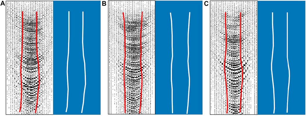
FIGURE 3. Three randomly seismic images (red lines, the boundaries manually picked) with their corresponding labels (with labeling ones, white line of Fresnel zones and zeros elsewhere) generated by manual interpretation.

FIGURE 4

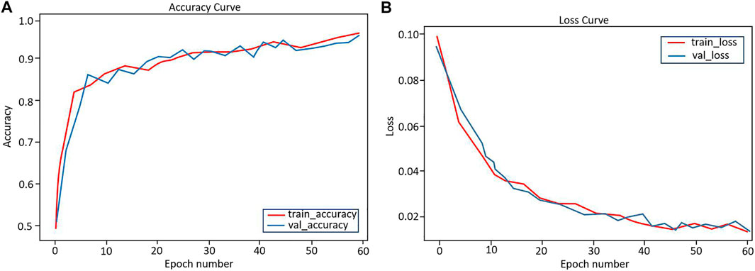
FIGURE 4. (A) The training and validation accuracy both will increase with epochs, whereas (B) the training and validation loss decreases with epochs.

4 Estimation of Effective $Q$

Zhang et al. (2013) introduced the definition of effective $Q$ , which is related to the spatial location of the imaging point with no knowledge of velocities, and proposed a constant $Q$ migration scanning method to obtain the effective $Q$ parameters. However, this method of obtaining $Q$ is complicated in calculation, and the quality of seismic data has a great influence on the accuracy of $Q$. We need a method that is more suitable for practical applications, taking into account both accuracy and efficiency. To address these issues, we develop an effective $Q$-model estimation scheme, and the specific implementation steps are as follows:

1) use VSP data to obtain initial $Q$ , expressed as $Q_{vsp}$. The number of VSP wells should be as many as possible, and the distribution should be as even as possible.

2) generate a synthetic trace without attenuation and different migrated traces with compensation. $Q$ is selected according to the match between the synthetic trace and their corresponding migrated traces and is denoted as $Q_{well}$.

3) use Lee’s empirical formula $Q=14v^{2.2}$ to get $Q$ from seismic data. The $Q$ is marked as $Q_{seismic}$. Lee’s empirical formula can quickly establish a Q model of the entire work area by using seismic velocity (Tian, 1990).

4) Use all $Q_{well}s$ to calibrate $Q_{seismic}$ and get a $Q$ model of the whole work area.

In step 1, we use the centroid frequency shift method (Quan and Harris, 1997) to estimate $Q$ that reads

$Q=\frac{\mathrm{\pi }\mathit{\tau }{\sigma }^2}{f_{shot}-f_{geo}},(6)$

where σ² is the variance of the source wavelet; τ is the travel time in the layers; and f_shot and f_geo are the centroid frequencies of the shot point and detection point, respectively. Since this method is sensitive to layering effects and background noise, it is necessary to preprocess the VSP data such as denoising. In addition, try to avoid thin layers, and select some large layers for $Q$ calculation.

In step 2, we use a Rick wavelet to generate a synthetic trace without attenuation at the location of this VSP well, first. Because the attenuation of shallow seismic data is weak, its dominant frequency can be used as the dominant frequency of the Rick wavelet. Next, we get different migrated imaging traces corresponding to the synthetic trace using PSTM with compensation under a set of regular variable $Q$. Based on $Q_{vsp}$ and multiplied by different weight coefficients, the variable $Q$ was obtained as 0.5, 0.6, 0.7, 0.8, 0.9,1.0, 1.1, 1.2, 1.3, 1.4, and 1.5 times of $Q_{vsp}$. The optimal $Q$ is selected according to the similarity between the synthetic trace and its corresponding seismic imaging traces.

In step 3, the unit of the parameter $v$ in Lee’s empirical formula is km/s, and it is a root mean square velocity. Lee’s formula uses velocity information to estimate the $Q$ value, which has the characteristics of high efficiency and easy realization in practical application. However, its estimation accuracy is low, and it needs to be corrected by well information.

In the last step, we use all $Q_{well}s$ to calibrate $Q_{seismic}$ and get a $Q$ model of the whole work area. $Q_{well}$ is derived from VSP data, and its accuracy is higher than that of $Q$ calculated from Lee’s formula. Using all $Q_{well}s$ to calibrate $Q_{seismic}$ can improve the overall accuracy of the $Q$ model.

5 Result

5.1 Field Data Example

In this section, we directly use a 2D field data line to analyze and discuss the effective $Q$ estimation, the identification of Fresnel zones using deep learning, and the imaging with compensation. This line consists of 1,000 CDPs (common depth point) with a CDP spacing of 12.5 m. The data are sampled at 1 ms with a length of 2.5 s.

Figure 5 shows how an optimal $Q$ value is obtained from the compensated imaging traces. The specific implementation process is as follows: we get the synthetic seismic trace without attenuation, and then use VSP data to estimate the $Q$ value, which is denoted as $Q_{vsp}$. Next, we get different migrated traces corresponding to the synthetic trace by PSTM with compensation using $Q_{vsp}$ with different weight coefficients. There are eleven weight coefficients used, which are 0.5, 0.6, 0.7, 0.8, 0.9, 1.0, 1.1, 1.2, 1.3, 1.4, and 1.5. Multiply $Q_{vsp}$ by different weight coefficients to obtain the waveforms of compensated imaging traces under different $Q$, and then, compare them with their corresponding synthetic seismic trace without attenuation. When the two waveforms are similar, the corresponding $Q$ value is the optimal $Q$. In Figure 5, trace 0 represents a synthetic seismic trace without attenuation, which exists as a reference trace during $Q$ picking. Trace 1 to trace 11 represent the compensated imaging traces under different $Q$. For example, trace 1 is when $Q_{vsp}$ is multiplied by 1.5, and trace 2 is when $Q_{vsp}$ is multiplied by 1.4, and so on; trace 11 is when $Q_{vsp}$ is multiplied by 0.5. On trace 0, six black typical crests are selected, and each crest is surrounded by a set of red dashed lines. The amplitude of the intersection of two red dashed lines with the wave curve is zero. These six crests represent six events. For each wave crest, two red dashed lines that envelop it extend from trace 0 to trace 11. We judge whether $Q$ is optimal according to whether the two red dashed lines intersect the wave curve at amplitude zero. The principle of picking $Q$ here is that when $Q$ is optimal, the waveform of its compensated imaging trace should be closest to that of its corresponding synthetic seismic trace without attenuation. The six red boxes in Figure 5 are the best $Q$-labeled. Figure 6 shows the final $Q$ model of real data, and the value is displayed as the reciprocal of $Q$.

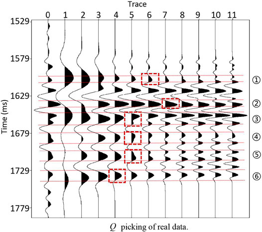
FIGURE 5

FIGURE 5. $Q$ picking of real data.

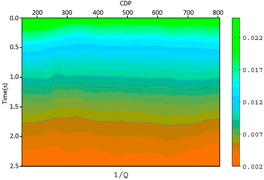
FIGURE 6

FIGURE 6. $Q$ model of real data.

Figure 7 shows part of the prediction results, which are the Fresnel zones predicted from the dip-angle gathers at three CDPs (400, 600, and 800). In order to solve the problem of local unsmoothness of Fresnel zones predicted by deep learning, the prediction results were sparsely processed and only twelve pairs of equally spaced sample points were retained. The Fresnel zones predicted by deep learning was obtained by connecting the sample points with smooth curves. In Figure 7, the red lines are the boundaries manually picked, while the green points on yellow lines are the sample points predicted by U-Net. The predicted boundaries of the Fresnel zones are similar to the manually picked ones, with a smoother curve. After superimposing the Fresnel zones at each CDP within the predicted boundaries, a migrated result with a higher S/N can be obtained. Figure 8 shows the compensated imaging results with different apertures. While Figure 9 shows the detailed comparison of two white boxes in Figure 8. The result with U-Net predicted an optimal aperture has a higher S/N than the result with a constant aperture. The prediction of each dip-angle gather by the trained U-Net requires approximately 0.6 s when using six TITAN Xp GPUs, which is much more efficient than manual picking. Figure 10 shows the comparison between the migration results obtained using conventional PSTM and the PSTM with compensation. The conventional PSTM used a constant aperture, and the compensated PSTM used an optimal aperture predicted by deep learning. Figure 11 shows the detailed comparison of two white boxes in Figure 10. We see the overlay events are well separated by the PSTM with compensation. Figure 12 shows the comparison of dB spectra between the migration sections obtained using conventional PSTM and the PSTM with compensation. The white boxes in Figure 10 are the time windows of the frequency spectrum. Observe that the high frequencies have been recovered well by the PSTM with compensation.

FIGURE 7

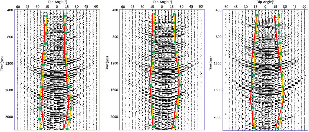
FIGURE 7. Prediction of the boundaries of the Fresnel zones from the dip-angle gathers at three CDPs (400, 600, and 800). The red lines are the boundaries manually picked, while the green points on yellow lines are the exact points predicted by U-Net. The predicted boundaries of the Fresnel zones are similar to the manually picked ones.

FIGURE 8

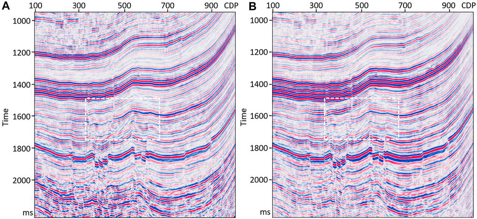
FIGURE 8. Comparison between the compensated migrated result with different apertures. Panel (A) represents the compensated migrated result with a constant aperture ranging from −17 to 17°, while panel (B) represents the result with the U-Net predicted optimal aperture. The result with the U-Net predicted optimal aperture has a higher S/N than the result with a constant aperture.

FIGURE 9

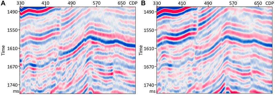
FIGURE 9. Comparison of the enlarged details inside the boxes of Figure 8. Panel (A) is the enlarged detail of the compensated migrated result with a constant aperture ranging from −17 to 17°, while panel (B) is that with the U-Net predicted optimal aperture.

FIGURE 10

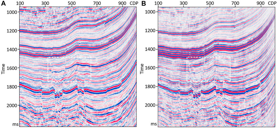
FIGURE 10. Comparison between the result obtained using conventional PSTM (A) and the result obtained using PSTM with compensating absorption and dispersion (B). Panel (A) represents the migrated result with a constant aperture ranging from −17 to 17°, while panel (B) represents the result with the U-Net predicted optimal aperture.

FIGURE 11

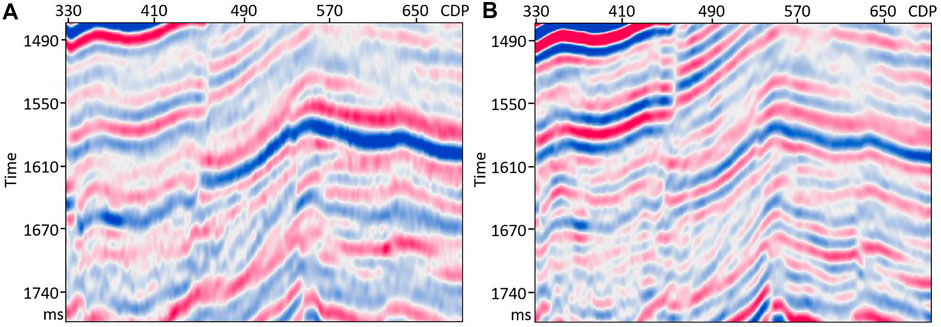
FIGURE 11. Comparison of the enlarged details in-side the boxes of Figure 10. Panel (A) is the enlarged detail of the conventional migrated result with a constant aperture ranging from −17 to 17°, while panel (B) is that of the compensated migrated result with the U-Net predicted optimal aperture.

FIGURE 12

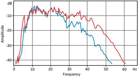
FIGURE 12. Comparison of amplitude spectra between the migration sections obtained using conventional PSTM (blue) and the PSTM with compensation (red).

6 Conclusion

We have presented a PSTM scheme that can compensate absorption and dispersion with effective $Q$ estimation and Fresnel zone identification based on deep learning. Using U-Net to estimate Fresnel zones from compensated migrated dip-angle gathers, we obtain an optimal migration aperture. The predicted boundaries of the Fresnel zones were similar to the manually picked ones, and the migrated result obtained by applying the predicted Fresnel zones exhibited a higher S/N. The effective $Q$ model is constructed using surface seismic velocity data and VSP well data. The optimal $Q$ is selected according to the similarity between the synthetic trace and its corresponding seismic imaging traces, which is a quick and effective method. Since the proposed migration scheme can compensate absorption and dispersion, the real data have been imaged with a higher resolution. Here, we discussed how to obtain 1D Fresnel zones from 1D dip-angle gathers for 2D seismic data using deep learning. Because of the high computation cost and memory requirement for 2D dip-angle gathers, it is difficult to directly estimate 2D Fresnel zones from 2D dip-angle gathers for 3D migration. Although 2D Fresnel zones can be represented by incorporating the inline and crossline 1D Fresnel zones from 1D dip-angle gathers obtained from 3D data, this simplified strategy will bring about inaccuracy of migration apertures in other directions except the inline and crossline directions. Therefore, it will be the next research focus to use deep learning to obtain 2D Fresnel zones from 3D data (Aki and Richards, 1980; Bleistein, 1984; Tian, 1990; Xu and Zhang, 2017; Wu and Zuo, 2019).

Data Availability Statement

The raw data supporting the conclusion of this article will be made available by the authors, without undue reservation.

Author Contributions

JW and YS contributed to conceptualization; JW and PL carried out the methodology; JW and AG helped with software; QY and JW performed validation; YS conducted the formal analysis; PL was responsible for investigation; AG and QY carried out data curation; JW wrote the original draft; JW was responsible for review and editing of the draft; QY carried out visualization; JW and PL was responsible for supervision. All authors have read and agreed to the published version of the manuscript.

Conflict of Interest

The authors declare that the research was conducted in the absence of any commercial or financial relationships that could be construed as a potential conflict of interest.

Publisher’s Note

All claims expressed in this article are solely those of the authors and do not necessarily represent those of their affiliated organizations, or those of the publisher, the editors, and the reviewers. Any product that may be evaluated in this article, or claim that may be made by its manufacturer, is not guaranteed or endorsed by the publisher.

Acknowledgments

The authors are grateful to the National Natural Science Foundation of China (41930431) and the China Postdoctoral Science Foundation (2020M680840) for supporting this work.

References

Aki, K., and Richards, P. G. (1980). Quantitative Seismology. W. H. Freeman.

Google Scholar

Bai, J., and Yingst, D.,“Q Estimation through Waveform Inversion,” in Proc. London, 75th EAGE Conf. Exhib. Incorporating SPE Europec, London, UK: Extended Abstr., 2013, 348-00601.doi:10.3997/2214-4609.20130112

CrossRef Full Text | Google Scholar

Bleistein, N. (1984). Mathematical Methods for Wave Phenomena. Academic Press.

Google Scholar

Brzostowski, M., and McMechan, G. (1992). 3-D Tomographic Imaging of Nearsurface Seismic Velocity and Attenuation. ”Geophysics 57 (3), 396–403. doi:10.1190/1.1443254

CrossRef Full Text | Google Scholar

Cavalca, M., Moore, I., Zhang, L., Ng, S. L., Fletcher, R., and Bayly, M. (2011). Ray-based Tomography for Q Estimation and Q Compensation in Complex media: 81st Annual International Meeting. Expanded Abstracts: SEG, 3989–3992.

Google Scholar

Chen, J. (2004). Specular ray Parameter Extraction and Stationary-phase Migration. Geophysics 69, 249–256. doi:10.1190/1.1649392

CrossRef Full Text | Google Scholar

Chen, Z., Chen, X., Wang, Y., and Jingye, L. (2014). Estimation of Q Factors from Reflection Seismic Data for a Band-Limited and Stabilized Inverse Q Filter Driven by an Average-Q Model. J. Appl. Geophys. 101, 86–94. doi:10.1016/j.jappgeo.2013.12.003

CrossRef Full Text | Google Scholar

Cheng, Q., Zhang, J., and Liu, W. (2020). Extracting Fresnel Zones from Migrated Dip-Angle Gathers Using a Convolutional Neural Network. Exploration Geophys. 52. 1-10. doi:10.1080/08123985.2020.1798755

CrossRef Full Text | Google Scholar

Dai, Y. U., Zhi-Jun, H. E., Yuan, S. U. N., and Wang, Y. A. (2018). A Comparison of the Inverse Q Filtering Methods Based on Wavefield continuation. J. Geophys. Geochem. Explor. 42 (2). 331–338.

Google Scholar

Dasgupta, R., and Clark, R. (1998). Estimation of Q from Surface Seismic Reflflection Data. Geophysics 63 (6), 2120–2128. doi:10.1190/1.1444505

CrossRef Full Text | Google Scholar

Dutta, G., and Schuster, G. (2016). Wave-equation Q Tomography. Geophysics 81 (6), R471–R484. doi:10.1190/geo2016-0081.1

CrossRef Full Text | Google Scholar

Ferber, R. (2005). A Filter Bank Solution to Absorption Simulation and Compensation: 75th Annual International Meeting. Expanded Abstracts: SEG, 2170–2172.

Google Scholar

Futterman, W. I. (1962). Dispersive Body Waves. J. Geophys. Res. 67 (13), 5279–5291. doi:10.1029/jz067i013p05279,

CrossRef Full Text | Google Scholar

Guo, P., McMechan, G. A., and Guan, H. (2016). Comparison of Two Viscoacoustic Propagators for Q-Compensated Reverse Time Migration. Geophys. J. Soc. Exploration Geophysicists 81 (5), S281–S297. doi:10.1190/geo2015-0557.1

CrossRef Full Text | Google Scholar

Hargreaves, N. D., and Calvert, A. J. (1991). Inverse Q Filtering by Fourier Transform. Geophysics 56, 519–527. doi:10.1190/1.1443067

CrossRef Full Text | Google Scholar

Hecht-Nielsen, R. (1989). Theory of the Backpropagation Neural Network. Neural Networks 11, 593–605. doi:10.1109/IJCNN.1989.118638

CrossRef Full Text | Google Scholar

Kamei, R., and Pratt, R. G., “Waveform Tomography Strategies for Imaging Attenuation Structure with Cross-Hole Data,” in Proc. 70th EAGE Conf. Exhib. Incorporating SPE EUROPEC, 2008.doi:10.3997/2214-4609.20147680

CrossRef Full Text | Google Scholar

Keers, H., Vasco, D. W., and Johnson, L. R. (2001). Viscoacoustic Crosswell Imaging Using Asymptotic Waveforms. Geophysics 66, 861–870. doi:10.1190/1.1444975

CrossRef Full Text | Google Scholar

Kingma, D. P., and Ba, J. (2014). Adam: A Method for Stochastic Optimization.

Google Scholar

Kjartansson, E. (1979). Constant Q Wave Propagation and Attenuation. J. Geophys. Res. 84 (1), 4737–4748. doi:10.1029/jb084ib09p04737

CrossRef Full Text | Google Scholar

Klokov, A., and Fomel, S. (2012a). Optimal Migration Aperturefor Conflicting Dips. 82nd Annual International Meeting. Expanded Abstracts: SEG.

Google Scholar

Klokov, A., and Fomel, S. (2012b). Separation and Imaging of Seismic Diffractions Using Migrated Dip-Angle Gathers. Geophysics 77 (6), S131–S143. doi:10.1190/geo2012-0017.1

CrossRef Full Text | Google Scholar

LeCun, Y., Bengio, Y., and Hinton, G. (2015). Deep learning. Nature 521, 436–444. doi:10.1038/nature14539

PubMed Abstract | CrossRef Full Text | Google Scholar

Li, Z., Zhang, J., and Liu, W. (2018). Diffraction Imaging Using Dipangle and Offset Gathers. Chin. J. Geophys. 61 (4), 1447–1459. doi:10.6038/cjg2018K0583

CrossRef Full Text | Google Scholar

Marfurt, K. J. (2006). Robust Estimates of 3D Reflector Dip and Azimuth. Geophysics 71 (4), P29–P40. doi:10.1190/1.2213049

CrossRef Full Text | Google Scholar

Neep, J., Worthington, M., and O’Hara-Dhand, K. (1996). Measurement of Seismic Attenuation from High-Resolution Crosshole Data. Geophysics 61 (4), 1175–1188. doi:10.1190/1.1444037

CrossRef Full Text | Google Scholar

Quan, Y., and Harris, J. M. (1997). Seismic Attenuation Tomography Using the Frequency Shift Method. Geophysics 62 (1), 895–905. doi:10.1190/1.1444197

CrossRef Full Text | Google Scholar

Ronneberger, O., Fischer, P., and Brox, T. (2015).U-net: Convolutional Networks for Biomedical Image Segmentation in MICCAI 2015. Editors N. Navab, J. Hornegger, W. M. Wells, and A. F. Frangi (Cham: LNCSSpringer), 9351, 234–241. doi:10.1007/978-3-319-24574-4_28

CrossRef Full Text | Google Scholar

Rumelhart, D. E., Hinton, G. E., and Williams, R. J. (1986c). Learning Representations by Back-Propagating Errors. Nature 323, 533–536. doi:10.1038/323533a0

CrossRef Full Text | Google Scholar

Sangwan, P., and Kumar, D. (2021). A Robust Approach to Estimate Q from Surface Seismic Data and Inverse Q Filtering for Resolution Enhancement. Houten, Netherlands: First Break.

Google Scholar

Schleicher, J., Hubral, P., Tygel, M., and Jaya, M. S. (1997). Minimum Apertures and Fresnel Zones in Migration and Demigration. Geophysics 62, 183–194. doi:10.1190/1.1444118

CrossRef Full Text | Google Scholar

Sevastopolsky, A. (2017). Optic Disc and Cup Segmentation Methods for Glaucoma Detection with Modification of U-Net Convolutional Neural Network. Pattern Recognition Image Anal. 27 (3), 618–624. doi:10.1134/s1054661817030269

CrossRef Full Text | Google Scholar

Shen, Y., Biondi, B., and Clapp, R.,“Q-model Building Using One-Way Wave-Equation Migration Q Analysis—Part 1: Theory and Synthetic Test,”Geophysics, 83, 2, 1–64. 2018. doi:10.1190/geo2016-0658.1

CrossRef Full Text | Google Scholar

Shen, Y., and Zhu, T. (2015). Image-based Q Tomography Using Reverse Time Q Migration. Proc. 85th Annu. Int. Meeting. Houston, TX: SEG, Expanded Abstr., 3694–3698. doi:10.1190/segam2015-5852526.1

CrossRef Full Text | Google Scholar

Shi, Y., Zhou, H.-L., Cong, N., Chun-Cheng, L., and Meng, L.-J. (2019). A Variable Gain-Limited Inverse. Q. Filtering Method Enhance Resolution Seismic data.Journal Seismic Exploration 28 (3), 257–276. 10.1190/obnobc2017-22.

Google Scholar

Smith, L. (2017). Cyclical Learning Rates for Training Neural Networks[C]. 2017 IEEE Winter Conference on Applications of Computer Vision (WACV). (IEEE).

Google Scholar

Tian, S. (1990). Estimating the Q Value in Inverse Q Filtering with Lee’s Empirical Formula. Pet. Geophys. Prospecting(in Chinese) 3, 354–361. doi:10.1111/1365-2478.12391

CrossRef Full Text | Google Scholar

Tieleman, T., and Hinton, G. (2012). Lecture 6.5-rmsprop: Divide the Gradient by a Running Average of its Recent Magnitude. COURSERA: Neural Networks for Machine Learning 4 (2).

Google Scholar

Tonn, R. (1991). The Determination of the Seismic Quality Factor Q from VSP Data: A Comparison of Different Computational Methods. Geophys. Prospecting 39 (1), 1–27. doi:10.1111/j.1365-2478.1991.tb00298.x

CrossRef Full Text | Google Scholar

Wang, Y. (2002). A Stable and Efficient Approach of Inverse Q Filtering. Geophysics 67, 657–663. doi:10.1190/1.1468627

CrossRef Full Text | Google Scholar

Wang, Y., Zhou, H., Chen, H., and Chen, Y. (2018). Adaptive Stabilization for Q-Compensated Reverse Time Migration. Geophysics. 83. 1-111. doi:10.1190/geo2017-0244.1

CrossRef Full Text | Google Scholar

Wu, J., Liu, B., Zhang, H., He, S., and Yang, Q. (2021). Fault Detection Based on Fully Convolutional Networks (FCN). J. Mar. Sci. Eng. 9 (3), 259. doi:10.3390/jmse9030259

CrossRef Full Text | Google Scholar

Wu, J., and Zuo, H. (2019). Attenuation Compensation in Prestack Time Migration and its GPU Implementation. Oil Geophys. Prospecting 54 (1), 84–92. doi:10.13810/j.cnki.issn.1000-7210.2019.01.010

CrossRef Full Text | Google Scholar

Wu, X., Liang, L., Shi, Y., and Fomel, S. (2019). FaultSeg3D: Using Synthetic Data Sets to Train an End-To-End Convolutional Neural Network for 3D Seismic Fault Segmentation. Geophysics 84, 35–45. doi:10.1190/geo2018-0646.1

CrossRef Full Text | Google Scholar

Xie, S. N., and Tu, Z. W. (2015). Holistically-Nested Edge Detection. Int. Conf. Comp. Vis. 1. 1395–1403. doi:10.1109/ICCV.2015.164

CrossRef Full Text | Google Scholar

Xie, Y., Xin, K., Sun, J., Notfors, C., Biswal, A. K., and Balasubramaniam, M. K. (2009). 3D prestack depth migration with compensation for frequency dependent absorption and dispersion: 79th Annual International Meeting. Expanded Abstracts. Houston, TX: SEG, 2919–2922. doi:10.1081/22020586.2010.12041885

CrossRef Full Text | Google Scholar

Xu, J., and Zhang, J. (2017). Prestack Time Migration of Nonplanar Data: Improving Topography Prestack Time Migration with Dip-Angle Domain Stationary-phase Filtering and Effective Velocity Inversion. Geophysics. 82 (3), S235–S246. doi:10.1190/geo2016-0087.1

CrossRef Full Text | Google Scholar

Yu, Z., Etgen, J., Whitcombe, D., Hodgson, L., and Liu, H. (2013).Dip-adaptive Operator Anti-aliasing for Kirchhoff Migration. 83rd Annual International Meeting. Expanded Abstracts. Houston, TX: SEG, 3692–3695. doi:10.1190/segam2013-0584.1

CrossRef Full Text | Google Scholar

Zhang, G., Wang, X., He, Z., Yu, G., Li, Y., Liu, W., et al. (2014). Impact of Q Value and Gain-Limit to the Resolution of Inverse Q Filtering. J. Geophys. Eng. 11(4), 45011. doi:10.1088/1742-2132/11/4/045011

CrossRef Full Text | Google Scholar

Zhang, H., Han, J., Li, Z., and Zhang, H. (2021). Extracting Q Anomalies from Marine Reflection Seismic Data Using Deep Learning. IEEE Geosci. Remote Sensing Lett. 1(99), 1–5. doi:10.1109/lgrs.2020.3048171

CrossRef Full Text | Google Scholar

Zhang, J. F., Wu, J. Z., and Li, X. Y. (2013). Compensation for Absorption and Dispersion in Prestack migration:An Effective Q Approach. Geophysics 78 (1), 1–14. doi:10.1190/geo2012-0128.1

CrossRef Full Text | Google Scholar

Zhang, J., and Wapenaar, K. (2002). Wavefield Extrapolation and Prestack Depth Migration in Anelastic Inhomogeneous media. Geophys. Prospecting 50 (1), 629–643. doi:10.1046/j.1365-2478.2002.00342.x

CrossRef Full Text | Google Scholar

Zhang, J., Li, Z., Liu, L., Wang, J., and Xu, J. (2016). High-resolution Imaging: An Approach by Incorporating Stationary-phase Implementation into Deabsorption Prestack Time Migration. Geophysics 81 (5), S317–S331. doi:10.1190/geo2015-0543.1

CrossRef Full Text | Google Scholar