Trapezoid-Grid Finite-Difference Time-Domain Method for 3D Seismic Wavefield Modeling Using CPML Absorbing Boundary Condition

The large computational memory requirement is an important issue in 3D large-scale wave modeling, especially for GPU calculation. Based on the observation that wave propagation velocity tends to gradually increase with depth, we propose a 3D trapezoid-grid finite-difference time-domain (FDTD) method to achieve the reduction of memory usage without a significant increase of computational time or a decrease of modeling accuracy. It adopts the size-increasing trapezoid-grid mesh to fit the increasing trend of seismic wave velocity in depth, which can significantly reduce the oversampling in the high-velocity region. The trapezoid coordinate transformation is used to alleviate the difficulty of processing ununiform grids. We derive the 3D acoustic equation in the new trapezoid coordinate system and adopt the corresponding trapezoid-grid convolutional perfectly matched layer (CPML) absorbing boundary condition to eliminate the artificial boundary reflection. Stability analysis is given to generate stable modeling results. Numerical tests on the 3D homogenous model verify the effectiveness of our method and the trapezoid-grid CPML absorbing boundary condition, while numerical tests on the SEG/EAGE overthrust model indicate that for comparable computational time and accuracy, our method can achieve about 50% reduction on memory usage compared with those on the uniform-grid FDTD method.

1 Introduction

Reverse time migration (RTM) (Baysal et al., 1983; Xuan et al., 2014; Qu et al., 2015; Xu et al., 2021a; Du et al., 2021) and full-waveform inversion (FWI) (Tarantola, 1984; Virieux and Operto, 2009; Cai and Zhang, 2015; Xia et al., 2017; Jia et al., 2019) play a fundamental role in geophysical exploration. Since forward modeling of the wave equation consumes most computational time in the RTM and FWI processes (Jing et al., 2019; Xu et al., 2021b; Liu et al., 2021), how to achieve the improvement of efficiency and the reduction of memory usage without a significant decrease of accuracy for 3D large-scale modeling is a key problem of seismic modeling. The finite-difference (FD) method has been regarded as one of the most popular wave modeling methods for its easy implementation and high-computational efficiency (Antunes et al., 2014; Abreu et al., 2015; Xu and Gao, 2018; Robertsson and Blanch, 2020). However, the numerical dispersion of the traditional FD method leads to the use of fine grids or high-order operators (Dablain, 1986; Liu and Sen, 2011b), which inevitably affects the efficiency of simulation.

The conventional FD method literally adopts a weighted summation of neighboring grid points’ values to estimate the derivative for a designated grid point (Zhou et al., 2021), where the grid size (h) is fixed and the FD coefficients are calculated by Taylor expansion. In this way, the approximation error ϵ can be expressed as (Liu and Sen, 2011a; Wu et al., 2019b) follows:

$ϵ=O{\left(\frac{hf}{v}\right)}^{2M},(1)$

where 2M is the length of the FD operator, h is the spatial interval, f is the frequency, and v is the seismic wave velocity. Considering that λ = v/f is the wavelength and G = λ/h is the number of grid points per wavelength (NPPW), we can rewrite Eq. 1 as follows:

$ϵ=O{\left(\frac{h}{\lambda }\right)}^{2M}=O{\left(\frac{1}{G}\right)}^{2M}.(2)$

Eq. 2 indicates that the modeling accuracy of the conventional FD method is proportional to G and M. Because the seismic wave velocity is varying in different positions, the wavelength is short in low-velocity regions and long in high-velocity regions (Liu, 2020). Therefore, a part of computing resources is wasted in the high-velocity regions for the fixed spatial interval and FD order. With respect to this problem, there are two kinds of techniques corresponding to the different understanding of Eq. 2. The first one is the variable-operator FD method (Liu and Sen, 2011a), which adopts the long and short FD stencils in the low- and high-velocity region, respectively. For the scheme in Liu and Sen (2011a), the variable-length FD stencils are designed by approaching the dispersion relation in the time–space domain, and Liu (2020) subsequently optimizes their FD coefficients.

The second one is the variable-grid FD method, which adopts different gird sizes in different regions and can efficiently reduce the oversampling in the high-velocity region. The key problem of the variable-grid FD method is the processing of the transition area between the fine grids and the coarse grids. The variable-grid FD method based on interpolation (Hayashi and Burns, 2005; Pasalic and McGarry, 2010) is the easiest one, in which the lacking information in the transition area is completed by interpolation. However, the resulting artificial reflection in the transition area and the possible instability make it inefficient for high-accuracy seismic wave simulation. Another variable-grid FD method adopts irregular FD coefficients to process the transition region (Huang and Dong, 2009; Liu et al., 2014), which can significantly avoid the artificial reflection and improve the stability. The disadvantage of this type of variable-grid method is the additional computing cost brought by calculating irregular FD coefficients.

The trapezoid-grid FD method (Chen and Xu, 2012; Gao et al., 2018; Wu et al., 2018, Wu et al., 2019a, Wu et al., 2019b) is one of the practical variable-grid methods. It uses the trapezoid-grid mesh to fit the trend of velocity increasing with depth, which can effectively reduce the number of required grid points. Meanwhile, the use of trapezoid coordinate transformation can avoid the difficulty of processing ununiform grids in the physical Cartesian coordinate system. On the other hand, the significant reduction of memory requirement of trapezoid-grid FDTD can improve the easy implementation of GPU calculation (Fujii et al., 2013; Li et al., 2016). The existing research on trapezoid-grid FDTD methods mainly focuses on 2D wavefield modeling. Therefore, it is essential to expand trapezoid-grid FDTD from 2D to 3D for realistic seismic exploration research.

In this article, we propose a 3D trapezoid-grid FDTD method for acoustic wave modeling. First, we design the 3D trapezoid coordinate transformation and derive the 3D acoustic equation in the trapezoid coordinate system. Second, to reduce the artificial boundary reflection (Ma et al., 2018, Ma et al., 2019), we apply the corresponding trapezoid-grid convolutional perfectly matched layer (CPML) absorbing boundary condition. Third, stability analysis is given to generate stable modeling results. We then test our proposed method on the 3D homogenous model and the SEG/EAGE overthrust model and compare the efficiency and accuracy of the trapezoid-grid FDTD method with the uniform-grid FDTD method. Finally, conclusions are shown in the last section.

2 Methods

2.1 3D Trapezoid Coordinate System

In this article, the 3D trapezoid coordinate transformation is defined as

$x=\frac{x_0-\alpha }{1+\gamma z_0};(\mathrm{3a})$

$y=\frac{y_0-\beta }{1+\gamma z_0};(\mathrm{3b})$

$z_0=g\left(z\right),(\mathrm{3c})$

where (x₀, y₀, z₀) is the Cartesian coordinate system, and (x, y, z) is the defined trapezoid coordinate system. In Eq. 3, α and β are central horizontal positions of the 3D trapezoid mesh, and γ is the scaling parameter for lateral coordinates. The velocity-related function g(z) is the sampling function for z₀-axis, which should be first- and second-order continuous for deriving 3D wave equations in the trapezoid coordinate system. The discrete points of g(z) are given by the following recursion:

$g\left(0\right)=0;(\mathrm{4a})$

$g\left(z+\mathrm{\Delta }z\right)=g\left(z\right)+\frac{v_{min}\left(g\left(z\right)\right)}{f_0{N}_0},(\mathrm{4b})$

where f₀ is the dominant frequency of the source term, N₀ is the preferred NPPW and is related to the accuracy of the adopted FD scheme, and v_min(g(z)) is the selected minimum velocity at depth g(z) in the physical Cartesian coordinate system and is smoothed by solving a local polynomial fitting problem with the constraint that v_min(g(z)) should not be greater than the model minimum velocity at depth g(z). The central value of each local polynomial corresponds to a value of v_min(g(z)). In particular, we usually set the order of the local polynomial as three. Such v_min(g(z)) can lead to a smooth sampling function g(z) for discontinuous velocity variation while satisfying the required number of points per wavelength in the z₀-direction.

If the grid sizes for the trapezoid-grid FDTD in the trapezoid coordinate system are defined as Δx, Δy, and Δz, then the corresponding grid sizes in the physical Cartesian system can be described as

$\mathrm{\Delta }{x}_0\left(z\right)=\left(1+\gamma g\left(z\right)\right)\mathrm{\Delta }x;(\mathrm{5a})$

$\mathrm{\Delta }{y}_0\left(z\right)=\left(1+\gamma g\left(z\right)\right)\mathrm{\Delta }y;(\mathrm{5b})$

$\mathrm{\Delta }{z}_0\left(z\right)=\frac{v_{min}\left(g\left(z\right)\right)}{f_0{N}_0}.(\mathrm{5c})$

In our work, γ and g(z) are determined adaptively according to the model velocity. By selecting γ such that Δx₀(z) and Δy₀(z) are always smaller than or equal to Δz₀(z), and a variable-grid mesh adaptive to the velocity model can be achieved in the physical Cartesian coordinate system. Figure 1 shows the schematic of the 3D trapezoid coordinate transform. Figure 1A shows the trapezoid-grid mesh in the Cartesian coordinate system, while Figure 1B shows the corresponding uniform grid mesh in the transformed trapezoid coordinate system. In particular, the two gray regions in Figure 1 represent the same physical region.

FIGURE 1

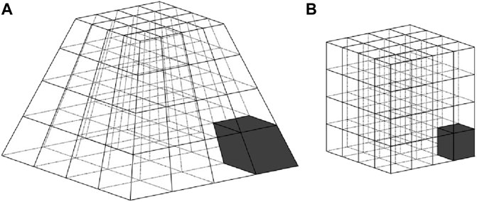
FIGURE 1. Schematic of the 3D trapezoid coordinate transformation: (A) the trapezoid-grid mesh in the Cartesian coordinate system; (B) the uniform grid mesh in the transformed trapezoid coordinate system. The two gray regions in A and B represent the same physical region.

2.2 3D Acoustic Equation with CPML Absorbing Boundary Condition in the Trapezoid Coordinate System

According to the theory of Pasalic and McGarry (2010), the time-domain-discretization form of the 3D isotropic acoustic equation with the CPML absorbing boundary condition in the Cartesian coordinate system can be described as

$\begin{array}{cc}\hfill & \frac{1}{v^2}\frac{u^{j+1}-2u^j+u^{j-1}}{\mathrm{\Delta }{t}^2}-\frac{{\partial }^2{u}^j}{\partial x_0^2}-\frac{{\partial }^2{u}^j}{\partial y_0^2}-\frac{{\partial }^2{u}^j}{\partial z_0^2}-\frac{\partial {\psi }_{x_0}^j}{\partial x_0}-\frac{\partial {\psi }_{y_0}^j}{\partial y_0}-\frac{\partial {\psi }_{z_0}^j}{\partial z_0}-{\zeta }_{x_0}^j-{\zeta }_{y_0}^j-{\zeta }_{z_0}^j\hfill \\ \hfill & =f\left(t_j\right)\delta \left(x_0-x_0^s\right)\delta \left(y_0-y_0^s\right)\delta \left(z_0-z_0^s\right);\hfill \end{array}(\mathrm{6a})$

${\psi }_{{\tau }_0}^{j+1}=a_{{\tau }_0}{\psi }_{{\tau }_0}^j+b_{{\tau }_0}\frac{\partial u^{j+1}}{\partial {\tau }_0};(\mathrm{6b})$

${\zeta }_{{\tau }_0}^{j+1}=a_{{\tau }_0}{\zeta }_{{\tau }_0}^j+b_{{\tau }_0}\left(\frac{{\partial }^2{u}^{j+1}}{\partial {\tau }_0^2}+\frac{\partial {\psi }_{{\tau }_0}^{j+1}}{\partial {\tau }_0}\right);(\mathrm{6c})$

$a_{{\tau }_0}=e^{-\left({\sigma }_{{\tau }_0}+{\alpha }_{{\tau }_0}\right)\mathrm{\Delta }t};(\mathrm{6d})$

$b_{{\tau }_0}=\frac{{\sigma }_{{\tau }_0}}{{\sigma }_{{\tau }_0}+{\alpha }_{{\tau }_0}}\left(a_{{\tau }_0}-1\right),{\tau }_0\in \left\{x_0,y_0,z_0\right\},(6e)$

where u^j = u(x₀, y₀, z₀, t_j) represents the scalar wavefield at the jth time step in the Cartesian coordinate system; v is the velocity; Δt is the time interval; f(t) is the source term; $(x_0^s,y_0^s,z_0^s)$ is the position of source; ${\sigma }_{{\tau }_0}=\frac{3v^{max}}{2L_{{\tau }_0}}{\left(\frac{{\bar{\tau }}_0}{L_{{\tau }_0}}\right)}^2$ln$\frac{1}{R}$, where R denotes the designated theoretical boundary reflection coefficient, v^max is the maximum velocity of the model, $L_{{\tau }_0}$ is the thickness of CPML absorbing boundary along the τ₀ direction, and ${\bar{\tau }}_0$ denotes the distance to the inner area in the τ₀ direction; ${\alpha }_{{\tau }_0}={\alpha }^{max}\left(1-\frac{{\bar{\tau }}_0}{L_{{\tau }_0}}\right)$ and α^max = πf₀.

In order to derive the acoustic equation in the trapezoid coordinate system, we first need to transform the derivatives in the Cartesian coordinate system into the derivatives in the trapezoid coordinate system. Based on the definition of the trapezoid coordinate system in Eq. 3 and the derivation rule of the composite function, the relationships of first- and second-order derivatives in the two coordinate systems can be given as

$\frac{\partial }{\partial x_0}=\frac{1}{1+\gamma g\left(z\right)}\frac{\partial }{\partial x};(\mathrm{7a})$

$\frac{\partial }{\partial y_0}=\frac{1}{1+\gamma g\left(z\right)}\frac{\partial }{\partial y};(\mathrm{7b})$

$\frac{\partial }{\partial z_0}=-\frac{\gamma x}{1+\gamma g\left(z\right)}\frac{\partial }{\partial x}-\frac{\gamma y}{1+\gamma g\left(z\right)}\frac{\partial }{\partial y}+\frac{1}{g^{\prime }\left(z\right)}\frac{\partial }{\partial z};(\mathrm{7c})$

$\frac{{\partial }^2}{\partial x_0^2}=\frac{1}{{\left[1+\gamma g\left(z\right)\right]}^2}\frac{{\partial }^2}{\partial x^2};(\mathrm{7d})$

$\frac{{\partial }^2}{\partial y_0^2}=\frac{1}{{\left[1+\gamma g\left(z\right)\right]}^2}\frac{{\partial }^2}{\partial y^2};(7e)$

$\begin{array}{cc}\hfill & \frac{{\partial }^2}{\partial z_0^2}=\frac{2{\gamma }^{2}x}{{\left[1+\gamma g\left(z\right)\right]}^2}\frac{\partial }{\partial x}+\frac{{\gamma }^2{x}^2}{{\left[1+\gamma g\left(z\right)\right]}^2}\frac{{\partial }^2}{\partial x^2}+\frac{2{\gamma }^{2xy}}{{\left[1+\gamma g\left(z\right)\right]}^2}\frac{{\partial }^2}{\partial x\partial y}\hfill \\ \hfill & -\frac{2\gamma x}{\left[1+\gamma g\left(z\right)\right]g^{\prime }\left(z\right)}\frac{{\partial }^2}{\partial x\partial z}+\frac{2{\gamma }^{2}y}{{\left[1+\gamma g\left(z\right)\right]}^2}\frac{\partial }{\partial y}+\frac{{\gamma }^2{y}^2}{{\left[1+\gamma g\left(z\right)\right]}^2}\frac{{\partial }^2}{\partial y^2}\hfill \\ \hfill & -\frac{2\gamma y}{\left[1+\gamma g\left(z\right)\right]g^{\prime }\left(z\right)}\frac{{\partial }^2}{\partial y\partial z}-\frac{g^{″}\left(z\right)}{{\left[g^{\prime }\left(z\right)\right]}^3}\frac{\partial }{\partial z}+\frac{1}{{\left[g^{\prime }\left(z\right)\right]}^2}\frac{{\partial }^2}{\partial z^2}\hfill \end{array}.(\mathrm{7f})$

Since the mixed spatial derivatives in Eq. 7f are hard to discrete directly with the FD method, to transform the mixed spatial derivatives into non-mixed spatial derivatives, we define three rotation transformations in the trapezoid coordinate system as

$\left[\begin{array}{c}\hfill x\hfill \\ \hfill z\hfill \end{array}\right]=\left[\begin{array}{cc}\hfill cos{\theta }_1\hfill & \hfill -sin{\theta }_1\hfill \\ \hfill sin{\theta }_1\hfill & \hfill cos{\theta }_1\hfill \end{array}\right]\left[\begin{array}{c}\hfill \widehat{x}\hfill \\ \hfill \widehat{z}\hfill \end{array}\right];(\mathrm{8a})$

$\left[\begin{array}{c}\hfill y\hfill \\ \hfill z\hfill \end{array}\right]=\left[\begin{array}{cc}\hfill cos{\theta }_2\hfill & \hfill -sin{\theta }_2\hfill \\ \hfill sin{\theta }_2\hfill & \hfill cos{\theta }_2\hfill \end{array}\right]\left[\begin{array}{c}\hfill \tilde{y}\hfill \\ \hfill \tilde{z}\hfill \end{array}\right];(\mathrm{8b})$

$\left[\begin{array}{c}\hfill x\hfill \\ \hfill y\hfill \end{array}\right]=\left[\begin{array}{cc}\hfill cos{\theta }_3\hfill & \hfill -sin{\theta }_3\hfill \\ \hfill sin{\theta }_3\hfill & \hfill cos{\theta }_3\hfill \end{array}\right]\left[\begin{array}{c}\hfill \bar{x}\hfill \\ \hfill \bar{y}\hfill \end{array}\right],(\mathrm{8c})$

where $\widehat{x}$ and $\widehat{z}$ are axes along diagonals in the (x, z) planes, $\tilde{y}$ and $\tilde{z}$ are axes along diagonals in the (y, z) planes, and $\bar{x}$ and $\bar{y}$ are axes along diagonals in the (x, y) planes. θ₁ is the angle between x and $\widehat{x}$ axes, θ₂ is the angle between y and $\tilde{y}$ axes, and θ₃ is the angle between x and $\bar{x}$ axes. A schematic of the coordinate transform in Eq. 8a is shown in Figure 2.

FIGURE 2

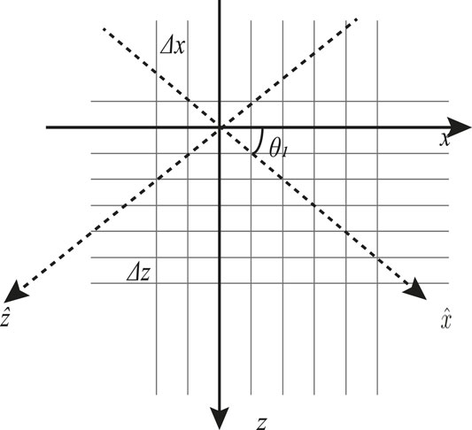
FIGURE 2. Schematic of the rotation transformation in the trapezoid coordinate system for transforming mixed spatial derivatives into non-mixed spatial derivatives.

By using Eqs. 8a–c, the mixed spatial derivatives in Eq. 7f can be transformed as

$\frac{{\partial }^2}{\partial x\partial z}=\frac{1}{2sin\left(2{\theta }_1\right)}\left(\frac{{\partial }^2}{\partial {\widehat{x}}^2}-\frac{{\partial }^2}{\partial {\widehat{z}}^2}\right);(\mathrm{9a})$

$\frac{{\partial }^2}{\partial y\partial z}=\frac{1}{2sin\left(2{\theta }_2\right)}\left(\frac{{\partial }^2}{\partial {\tilde{y}}^2}-\frac{{\partial }^2}{\partial {\tilde{z}}^2}\right);(\mathrm{9b})$

$\frac{{\partial }^2}{\partial x\partial y}=\frac{1}{2sin\left(2{\theta }_3\right)}\left(\frac{{\partial }^2}{\partial {\bar{x}}^2}-\frac{{\partial }^2}{\partial {\bar{y}}^2}\right).(\mathrm{9c})$

For simplicity, we usually use equal grid sizes in the trapezoid coordinate system (Δx = Δy = Δz = Δ), which means ${\theta }_1={\theta }_2={\theta }_3=\frac{\pi }{4}$. By substituting Eq. 7 and Eq. 9 into Eq. 6, we get the time-domain-discretization form of the 3D acoustic equation with the CPML absorbing boundary condition in the trapezoid coordinate system as

$\begin{array}{cc}\hfill & \frac{1}{v^2}\frac{u^{j+1}-2u^j+u^{j-1}}{\mathrm{\Delta }{t}^2}-\frac{{\gamma }^2{x}^2+1}{{\left[1+\gamma g\left(z\right)\right]}^2}\frac{{\partial }^2{u}^j}{\partial x^2}-\frac{{\gamma }^2{y}^2+1}{{\left[1+\gamma g\left(z\right)\right]}^2}\frac{{\partial }^2{u}^j}{\partial y^2}-\frac{2{\gamma }^{2}x}{{\left[1+\gamma g\left(z\right)\right]}^2}\frac{\partial u^j}{\partial x}\hfill \\ \hfill & -\frac{2{\gamma }^{2}y}{{\left[1+\gamma g\left(z\right)\right]}^2}\frac{\partial u^j}{\partial y}+\frac{\gamma x}{\left[1+\gamma g\left(z\right)\right]g^{\prime }\left(z\right)}\left(\frac{{\partial }^2{u}^j}{\partial {\widehat{x}}^2}-\frac{{\partial }^2{u}^j}{\partial {\widehat{z}}^2}\right)+\frac{\gamma y}{\left[1+\gamma g\left(z\right)\right]g^{\prime }\left(z\right)}\left(\frac{{\partial }^2{u}^j}{\partial {\tilde{y}}^2}-\frac{{\partial }^2{u}^j}{\partial {\tilde{z}}^2}\right)\hfill \\ \hfill & -\frac{{\gamma }^{2}xy}{{\left[1+\gamma g\left(z\right)\right]}^2}\left(\frac{{\partial }^2{u}^j}{\partial {\bar{x}}^2}-\frac{{\partial }^2{u}^j}{\partial {\bar{y}}^2}\right)+\frac{g^{″}\left(z\right)}{{\left[g^{\prime }\left(z\right)\right]}^3}\frac{\partial u^j}{\partial z}-\frac{1}{{\left[g^{\prime }\left(z\right)\right]}^2}\frac{{\partial }^2{u}^j}{\partial z^2}-\frac{1}{1+\gamma g\left(z\right)}\frac{\partial {\psi }_x^j}{\partial x}\hfill \\ \hfill & -\frac{1}{1+\gamma g\left(z\right)}\frac{\partial {\psi }_y^j}{\partial y}+\frac{\gamma x}{1+\gamma g\left(z\right)}\frac{\partial {\psi }_z^j}{\partial z}+\frac{\gamma y}{1+\gamma g\left(z\right)}\frac{\partial {\psi }_z^j}{\partial y}-\frac{1}{g^{\prime }\left(z\right)}\frac{\partial {\psi }_z^j}{\partial z}-{\zeta }_x^j-{\zeta }_y^j-{\zeta }_z^j\hfill \\ \hfill & =f\left(t_j\right)\left(x-x^s\right)\left(y-y^s\right)\left(z-z^s\right);\hfill \end{array}(\mathrm{10a})$

${\psi }_x^{j+1}=a_x{\psi }_x^j+b_x\frac{1}{1+\gamma g\left(z\right)}\frac{\partial u^{j+1}}{\partial x};(\mathrm{10b})$

${\psi }_y^{j+1}=a_y{\psi }_y^j+b_y\frac{1}{1+\gamma g\left(z\right)}\frac{\partial u^{j+1}}{\partial y};(\mathrm{10c})$

${\psi }_z^{j+1}=a_z{\psi }_z^j+b_z\left(-\frac{\gamma x}{1+\gamma g\left(z\right)}\frac{\partial u^{j+1}}{\partial x}-\frac{\gamma y}{1+\gamma g\left(z\right)}\frac{\partial u^{j+1}}{\partial y}+\frac{1}{g^{\prime }\left(z\right)}\frac{\partial u^{j+1}}{\partial z}\right);(\mathrm{10d})$

${\zeta }_x^{j+1}=a_x{\zeta }_x^j+b_x\left(\frac{1}{{\left[1+\gamma g\left(z\right)\right]}^2}\frac{{\partial }^2{u}^{j+1}}{\partial x^2}+\frac{1}{1+\gamma g\left(z\right)}\frac{\partial {\psi }_x^{j+1}}{\partial x}\right);(10e)$

${\zeta }_y^{j+1}=a_y{\zeta }_y^j+b_y\left(\frac{1}{{\left[1+\gamma g\left(z\right)\right]}^2}\frac{{\partial }^2{u}^{j+1}}{\partial y^2}+\frac{1}{1+\gamma g\left(z\right)}\frac{\partial {\psi }_y^{j+1}}{\partial y}\right);(\mathrm{10f})$

$\begin{array}{cc}\hfill & {\zeta }_z^{j+1}=a_z{\zeta }_z^j+b_z\left[\frac{{\gamma }^2{x}^2}{{\left[1+\gamma g\left(z\right)\right]}^2}\frac{{\partial }^2{u}^{j+1}}{\partial x^2}+\frac{{\gamma }^2{y}^2}{{\left[1+\gamma g\left(z\right)\right]}^2}\frac{{\partial }^2{u}^{j+1}}{\partial y^2}+\frac{2{\gamma }^{2}x}{{\left[1+\gamma g\left(z\right)\right]}^2}\frac{\partial u^{j+1}}{\partial x}\right.\hfill \\ \hfill & +\frac{2{\gamma }^{2}y}{{\left[1+\gamma g\left(z\right)\right]}^2}\frac{\partial u^{j+1}}{\partial y}-\frac{\gamma x}{\left[1+\gamma g\left(z\right)\right]g^{\prime }\left(z\right)}\left(\frac{{\partial }^2{u}^{j+1}}{\partial {\widehat{x}}^2}-\frac{{\partial }^2{u}^{j+1}}{\partial {\widehat{z}}^2}\right)\hfill \\ \hfill & -\frac{\gamma y}{\left[1+\gamma g\left(z\right)\right]g^{\prime }\left(z\right)}\left(\frac{{\partial }^2{u}^{j+1}}{\partial {\tilde{y}}^2}-\frac{{\partial }^2{u}^{j+1}}{\partial {\tilde{z}}^2}\right)+\frac{{\gamma }^{2}xy}{{\left[1+\gamma g\left(z\right)\right]}^2}\left(\frac{{\partial }^2{u}^{j+1}}{\partial {\bar{x}}^2}-\frac{{\partial }^2{u}^{j+1}}{\partial {\bar{y}}^2}\right)\hfill \\ \hfill & -\frac{g^{″}\left(z\right)}{{\left[g^{\prime }\left(z\right)\right]}^3}\frac{\partial u^{j+1}}{\partial z}+\frac{1}{{\left[g^{\prime }\left(z\right)\right]}^2}\frac{{\partial }^2{u}^{j+1}}{\partial z^2}-\frac{\gamma x}{1+\gamma g\left(z\right)}\frac{\partial {\psi }_z^{j+1}}{\partial x}-\frac{\gamma y}{1+\gamma g\left(z\right)}\frac{\partial {\psi }_z^{j+1}}{\partial y}+\frac{1}{g^{\prime }\left(z\right)}\frac{\partial {\psi }_z^{j+1}}{\partial z}],\hfill \end{array}(\mathrm{10g})$

where u^j = u(x, y, z, t_j) represents the scalar wavefield at the jth time step in the trapezoid coordinate system; (x^s, y^s, z^s) is the position of the source in the trapezoid coordinate system; ${\sigma }_{\tau }=\frac{3v^{max}}{2L_{\tau }}{\left(\frac{\bar{\tau }}{L_{\tau }}\right)}^2$ln$\frac{1}{R}$, where L_τ is the thickness of CPML absorbing boundary along the τ direction, $\bar{\tau }$ denotes the distance to the inner area in the τ direction; and ${\alpha }_{\tau }={\alpha }^{max}\left(1-\frac{\bar{\tau }}{L_{\tau }}\right)$, τ ∈ {x, y, z}.

A schematic of the grid discretization in the 3D trapezoid-grid CPML area is shown in Figure 3. In this work, 30 and 20 absorbing boundary layers are usually used for the trapezoid-grid CPML area in the horizontal and vertical directions, respectively.

FIGURE 3

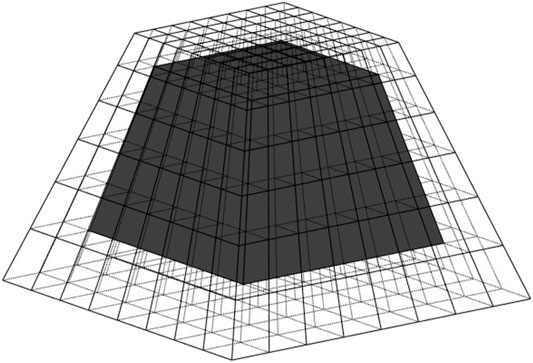
FIGURE 3. Schematic of the grid discretization in the 3D trapezoid-grid CPML area.

2.3 Stability Analysis

Stability condition is usually required for the FD scheme to give a stable time step. From Eq. 10a, we use a local frozen coefficients technique in each discrete point and can get the full-discretization form of the 3D trapezoid coordinate system acoustic equation without the CPML boundary condition and source function:

$\begin{array}{cc}\hfill & \frac{1}{v^2}\frac{u_{m,n,l}^{j+1}-2u_{m,n,l}^j+u_{m,n,l}^{j-1}}{\mathrm{\Delta }{t}^2}-\frac{{\gamma }^2{x}_m^2+1}{{\left[1+\gamma g\left(z_l\right)\right]}^2}\frac{1}{{\mathrm{\Delta }}^2}\sum _{p=1}^{N_x}{\eta }_p^x\left(u_{m-p,n,l}^j-2u_{m,n,l}^j+u_{m+p,n,l}^j\right)\hfill \\ \hfill & -\frac{{\gamma }^2{y}_n^2+1}{{\left[1+\gamma g\left(z_l\right)\right]}^2}\frac{1}{{\mathrm{\Delta }}^2}\sum _{p=1}^{N_y}{\eta }_p^y\left(u_{m,n-p,l}^j-2u_{m,n,l}^j+u_{m,n+p,l}^j\right)\hfill \\ \hfill & -\frac{2{\gamma }^2{x}_m}{{\left[1+\gamma g\left(z_l\right)\right]}^2}\frac{1}{\mathrm{\Delta }}\sum _{p=1}^{N_x}{c}_p^x\left(u_{m+p,n,l}^j-u_{m-p,n,l}^j\right)-\frac{2{\gamma }^2{y}_n}{{\left[1+\gamma g\left(z_l\right)\right]}^2}\frac{1}{\mathrm{\Delta }}\sum _{p=1}^{N_y}{c}_p^y\left(u_{m,n+p,l}^j-u_{m,n-p,l}^j\right)\hfill \\ \hfill & +\frac{\gamma x_m}{\left[1+\gamma g\left(z_l\right)\right]g^{\prime }\left(z_l\right)}\frac{1}{2{\mathrm{\Delta }}^2}\sum _{p=1}^{N_{xz}}{\eta }_p^{xz}\left(u_{m-p,n,l-p}^j+u_{m+p,n,l+p}^j-u_{m-p,n,l+p}^j-u_{m+p,n,l-p}^j\right)\hfill \\ \hfill & +\frac{\gamma y_n}{\left[1+\gamma g\left(z_l\right)\right]g^{\prime }\left(z_l\right)}\frac{1}{2{\mathrm{\Delta }}^2}\sum _{p=1}^{N_{yz}}{\eta }_p^{yz}\left(u_{m,n-p,l-p}^j+u_{m,n+p,l+p}^j-u_{m,n-p,l+p}^j-u_{m,n+p,l-p}^j\right)\hfill \\ \hfill & -\frac{{\gamma }^2{x}_m{y}_n}{{\left[1+\gamma g\left(z_l\right)\right]}^2}\frac{1}{2{\mathrm{\Delta }}^2}\sum _{p=1}^{N_{xy}}{\eta }_p^{xy}\left(u_{m-p,n-p,l}^j+u_{m+p,n+p,l}^j-u_{m-p,n+p,l}^j-u_{m+p,n-p,l}^j\right)\hfill \\ \hfill & +\frac{g^{″}\left(z_l\right)}{{\left[g^{\prime }\left(z_l\right)\right]}^3}\frac{1}{\mathrm{\Delta }}\sum _{p=1}^{N_z}{c}_p^z\left(u_{m,n,l+p}^j-u_{m,n,l-p}^j\right)-\frac{1}{{\left[g^{\prime }\left(z_l\right)\right]}^2}\frac{1}{{\mathrm{\Delta }}^2}\sum _{p=1}^{N_z}{\eta }_p^z\left(u_{m,n,l-p}^j-2u_{m,n,l}^j+u_{m,n,l+p}^j\right)=0\hfill \end{array},(11)$

where $u_{m,n,l}^j$ is the wavefield at (x_m, y_n, z_l, t_j), x_m = x⁰ + (m − 1)Δx, y_n = y⁰ + (n − 1)Δy, z_l = z⁰ + (l − 1)Δz, t_j = t⁰ + (j − 1)Δt, N_x, N_y, N_z, N_xy, N_xz, N_yz are half-of-spatial FD orders, η^x, η^y, η^z, η^xy, η^xz, η^yz are corresponding FD coefficients of the second-order derivative, and c^x, c^y, c^z, c^xy, c^xz, c^yz are corresponding FD coefficients of the first-order derivative.

To derive the stability condition, we use the plane wave solution that is defined as

$u\left(x,y,z,t\right)=u_0^{*}{e}^{i\omega t-i{k}_{x}x-i{k}_{y}y-i{k}_{z}z},(12)$

where $u_0^{*}$ is the amplitude of the plane wave, i is the imaginary unit, ω is the angular frequency, and k_x, k_y, k_z are wavenumbers in the x-, y- and z-directions, respectively. Similar to stability analysis of Kosloff and Baysal (1982), by substituting Eq. 12 into Eq. 11 and only considering the maximum wavenumber, the stability condition of the 3D acoustic equation in the trapezoid coordinate system can be expressed as

$\begin{array}{c}\hfill \mathrm{\Delta }t<\frac{\mathrm{\Delta }}{v^{max}}\underset{m,n,l}{max}{\left(\frac{{\gamma }^2{x}_m^2+1}{{\left[1+\gamma g\left(z_l\right)\right]}^2}\sum _{p=1}^{N_x}mod\left(p,2\right){\eta }_p^x+\frac{{\gamma }^2{y}_n^2+1}{{\left[1+\gamma g\left(z_l\right)\right]}^2}\sum _{p=1}^{N_y}mod\left(p,2\right){\eta }_p^y+\frac{1}{{\left[g^{\prime }\left(z_l\right)\right]}^2}\sum _{p=1}^{N_z}mod\left(p,2\right){\eta }_p^z\right)}^{-\frac{1}{2}}\hfill \end{array},(13)$

where mod is the function for the getting remainder, and $\underset{m,n,l}{max}$ represents the maximum value of the objective function at those discrete points (x_m, y_n, z_l).

3 Numerical Results

In the following numerical examples, Eq. 10 is discretized by the eighth-order FD in the space, and conventional Taylor-expansion–based high-order FD coefficients (Dablain, 1986) are adopted.

3.1 Homogenous Model

First, we use a 3D homogenous model with a constant velocity of 2000 m/s to verify the effectiveness of our trapezoid-grid FDTD method and corresponding CPML absorbing boundary condition. A Ricker wavelet with a dominant frequency of 20 Hz is located at the center of the model as the source. The FD time step is taken as 1.6 ms. The scaling parameter γ is set as 2.78 × 10^–4, the sampling function g(z) = z, and the lateral grid sizes in the Cartesian coordinate system increase from 7.5 to 10 from top to bottom. Figure 4A shows the snapshot obtained by the trapezoid-grid FDTD with CPML at 0.45 s, while Figure 4B shows the corresponding snapshot without CPML. Figure 5 shows the comparison between the recorded seismograms computed by the uniform-grid FDTD and the trapezoid-grid FDTD at (x₀, y₀, z₀) = (600, 600, 0 m). The comparison between Figures 4A,B demonstrates that trapezoid-grid CPML can effectively reduce boundary reflections, while Figure 5 demonstrates the accuracy of the trapezoid-grid FDTD method for the homogenous model.

FIGURE 4

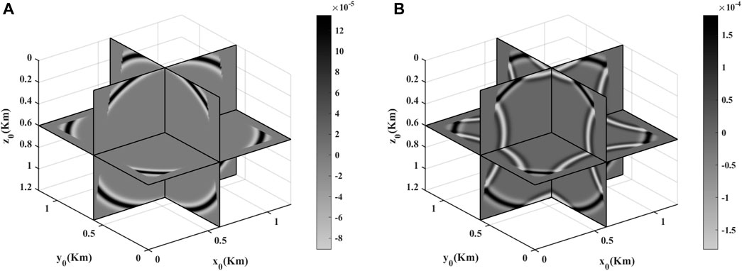
FIGURE 4. Snapshots obtained by the trapezoid-grid FDTD for the homogenous model (A) with CPML and (B) without CPML.

FIGURE 5

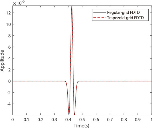
FIGURE 5. Comparison of seismograms obtained by the uniform-grid FDTD and the trapezoid-grid FDTD for the homogenous model at (x₀, y₀, z₀) = (600 m, 600 m, 0 m). The black solid line represents the uniform-grid FDTD result, and the red dash line represents the trapezoid-grid FDTD result.

3.2 Overthrust Model

Then, we apply our method to the SEG/EAGE overthrust model (Figure 6A), which is based on the real overthrusts of South America. Figures 6B,C show the modeling area of the SEG/EAGE overthrust model in the trapezoid coordinate system and the Cartesian coordinate system, respectively. A Ricker wavelet with the dominate frequency of 4.2 Hz is located at (10 km, 10 km, 0.5 km) as the source. The grid sizes for the uniform-grid FDTD are 50 m × 50 m × 50 m, which means the minimum NPPW in each direction is close to 10. We therefore set the minimum NPPW in x₀-, y₀-, and z₀-direction as 10 for the trapezoid-grid FDTD method, and get the scaling parameter as γ = 2.07 × 10^–4. Figure 7A shows the vertical sampling function g(z) used for this model, and the vertical grid sizes in the Cartesian coordinate system increase from 51.8 m in the shallow region to a maximum value of 142.6 m in the deep region, as shown in Figure 7B. Based on the stability analysis, the time step for the trapezoid-grid FDTD and the uniform-grid FDTD are 3.697 and 3.585 ms, respectively. Receivers are located on the surface along y₀ = 10 km. Figure 8A shows the snapshot at 2.5 s computed by the uniform-grid FDTD, and Figure 8B is the snapshot at 2.5 s in the trapezoid coordinate system computed by our trapezoid-grid method. Using coordinate transformation and cubic spline interpolation, we can get the corresponding snapshot in the Cartesian coordinate system, as shown in Figure 8C. Figures 8A,C show good agreement. To give more detailed comparisons, single-trace seismograms at (7.5, 10, 0 km), (10, 10, 0 km), and (12.5, 10, 0 km) for both the uniform-grid (black solid line) and the trapezoid-grid (red dash line) FDTD are shown in Figure 9. Figure 9 also shows good agreement between the uniform-gird FDTD and the trapezoid-grid FDTD. On our computing platform (Intel(R) Xeon(R) Sliver 4216 CPU @ 2.10GHz, 256GB of memory, and C++ codes), using 16-threads computation and similar code optimization techniques, the running time for the trapezoid-grid FDTD and the uniform-grid FDTD is calculated as 2203 s and 2925 s, respectively, which shows a calculation efficiency improvement of 24.7%. The memories for the trapezoid-grid FDTD and the uniform-grid FDTD are about 336 and 1213 MB, respectively, which shows a memory reduction of 72.3%. Considering that the simulation area of our trapezoid-grid method is almost 60% of that of the uniform-grid method, for the common simulation area, we can achieve about 50% reduction on memory usage.

FIGURE 6

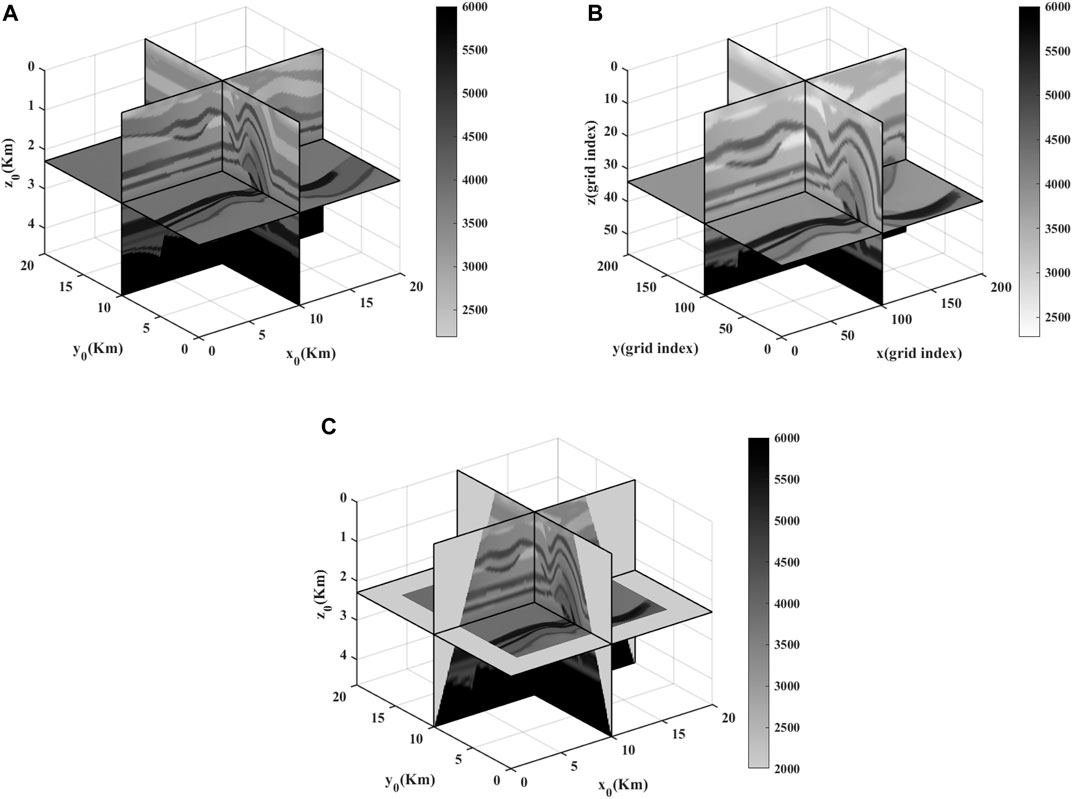
FIGURE 6. (A) SEG/EAGE overthrust model; (B) SEG/EAGE overthrust model in the trapezoid coordinate system; (C) actual simulating area for the trapezoid-grid FDTD in the Cartesian coordinate system.

FIGURE 7

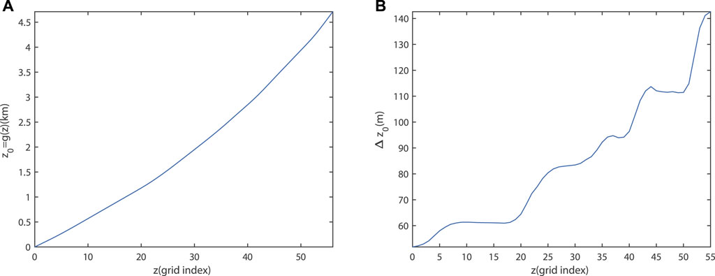
FIGURE 7. (A) Vertical sampling function g(z); (B) variation of Δz₀ for the trapezoid-grid FDTD.

FIGURE 8

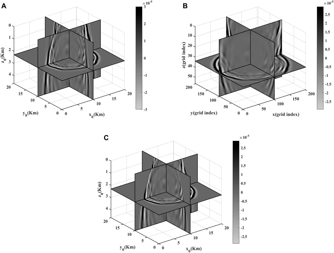
FIGURE 8. Snapshots for the SEG/EAGE overthrust model at 2.5 s: (A) uniform-grid FDTD result; (B) trapezoid-grid FDTD result in the trapezoid coordinate system; (C) trapezoid-grid FDTD result in the Cartesian coordinate system.

FIGURE 9

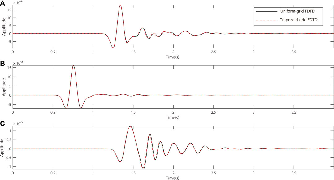
FIGURE 9. Single-trace seismograms for the SEG/EAGE overthrust model at the receiver position of (A) (7.5, 10, 0 km); (B) (10, 10, 0 km); and (C) (12.5, 10, 0 km). The black solid lines represent the uniform-grid FDTD results, and the red dash lines represent the trapezoid-grid FDTD results.

4 Conclusion

In this article, we propose a 3D trapezoid-grid FDTD seismic wave modeling method based on the increasing trend of seismic wave velocity with depth. The trapezoid-grid mesh in the physical Cartesian system can effectively reduce the oversampling in the high-velocity region compared with the uniform-grid method, and the design of 3D trapezoid coordinate transform greatly avoids the difficulty of processing an irregular grid. We derive the 3D acoustic equation in the trapezoid coordinate system. The corresponding CPML boundary condition is also given to decrease artificial boundary reflection. To obtain a stable and efficient wave modeling result, we combine the plane wave theory and frozen coefficients technique and provide an effective stability condition for the 3D trapezoid-grid FDTD method. The discretization of the 3D acoustic equation in the trapezoid coordinate system is completed by the eighth order and second order finite-difference method in the space and time domain, respectively. The 3D homogenous model is given to verify the effectiveness of trapezoid-grid FDTD and the performance of the CPML boundary. Numerical tests on the SEG/EAGE overthrust model indicate the accuracy and the significant memory reduction of our method compared with uniform-grid FDTD. The key idea of our method is the combination of the trapezoid coordinate transformation and the FD stencils. Such idea can be generalized to many other wave equations such as elastic equation (Zhan et al., 2017) and Maxwell’s equations (Zhan et al., 2021). Besides, our method is actually dealing with the regular grids in the trapezoid coordinate system, which means that we can combine other methods to treat the irregular surface (Li et al., 2020) or curved interfaces (Zhan et al., 2020).

Data Availability Statement

The original contributions presented in the study are included in the article/Supplementary Material; further inquiries can be directed to the corresponding author.

Author Contributions

BW contributed to the conception of the study. Writing, compiling, and debugging of the program were completed by WX. WT wrote the first draft of the manuscript, and all authors contributed to the revision.

Funding

We would like to thank the Natural Science Foundation of Shaanxi Province under Grant No. 2020JM-018 and National Natural Science Foundation (41974122) of China for funding this work.

Conflict of Interest

Authors BW, WT, and BL are employed by SINOPEC.

The remaining authors declare that the research was conducted in the absence of any commercial or financial relationships that could be construed as a potential conflict of interest.

Publisher’s Note

All claims expressed in this article are solely those of the authors and do not necessarily represent those of their affiliated organizations, or those of the publisher, the editors, and the reviewers. Any product that may be evaluated in this article, or claim that may be made by its manufacturer, is not guaranteed or endorsed by the publisher.

References

Abreu, R., Stich, D., and Morales, J. (2015). The Complex-Step-Finite-Difference Method. Geophys. J. Int. 202, 72–93. doi:10.1093/gji/ggv125

CrossRef Full Text | Google Scholar

Antunes, A. J. M., Leal-Toledo, R. C. P., Filho, O. T. d. S., and Toledo, E. M. (2014). Finite Difference Method for Solving Acoustic Wave Equation Using Locally Adjustable Time-Steps. Proced. Computer Sci. 29, 627–636. doi:10.1016/j.procs.2014.05.056

CrossRef Full Text | Google Scholar

Baysal, E., Kosloff, D. D., and Sherwood, J. W. C. (1983). Reverse Time Migration. Geophysics 48, 1514–1524. doi:10.1190/1.1441434

CrossRef Full Text | Google Scholar

Cai, J., and Zhang, J. (2015). “Acoustic Full Waveform Inversion with Physical Model Data,” in 2015 Workshop: Depth Model Building: Full-Waveform Inversion. Beijing, China: Society of Exploration Geophysicists (SEG), 146–149. doi:10.1190/FWI2015-036

CrossRef Full Text | Google Scholar

Chen, F., and Xu, S. (2012). “Pyramid-shaped Grid for Elastic Wave Propagation,” in SEG Technical Program Expanded Abstracts 2012 (Las Vegas: Society of Exploration Geophysicists (SEG)), 1–5. doi:10.1190/segam2012-0890.1

CrossRef Full Text | Google Scholar

Dablain, M. A. (1986). The Application of High‐order Differencing to the Scalar Wave Equation. GEOPHYSICS 51, 54–66. doi:10.1190/1.1442040

CrossRef Full Text | Google Scholar

Du, Q., Zhang, X., Zhang, S., Zhang, F., and Fu, L.-Y. (2021). The Pseudo-laplace Filter for Vector-Based Elastic Reverse Time Migration. Front. Earth Sci. 9, 538. doi:10.3389/feart.2021.687835

CrossRef Full Text | Google Scholar

Fujii, Y., Azumi, T., Nishio, N., Kato, S., and Edahiro, M. (2013). “Data Transfer Matters for Gpu Computing” in Proceeding of the 2013 International Conference on Parallel and Distributed Systems, Seoul, Korea (South), 15-18 Dec. 2013, (IEEE), 275–282. doi:10.1109/ICPADS.2013.47

CrossRef Full Text | Google Scholar

Gao, J., Xu, W., Wu, B., Li, B., and Zhao, H. (2018). Trapezoid Grid Finite Difference Seismic Wavefield Simulation with Uniform Depth Sampling Interval. Chin. J. Geophys. 61, 3285–3296. doi:10.6038/cjg2018M0313

CrossRef Full Text | Google Scholar

Hayashi, K., and Burns, D. R. (1999). “Variable Grid Finite‐difference Modeling Including Surface Topography,” in SEG Technical Program Expanded Abstracts 1999 (Houston: Society of Exploration Geophysicists (SEG)), 528–531. doi:10.1190/1.1821071

CrossRef Full Text | Google Scholar

Hong-Qiao, X., Xiao-Yi, W., Chen-Yuan, W., and Jiang-Jie, Z. (2021a). Sparse Constrained Least-Squares Reverse Time Migration Based on Kirchhoff Approximation. Front. Earth Sci. 9, 770. doi:10.3389/feart.2021.731697

CrossRef Full Text | Google Scholar

Huang, C., and Dong, L.-G. (2009). Staggered-Grid High-Order Finite-Difference Method in Elastic Wave Simulation with Variable Grids and Local Time-Steps. Chin. J. Geophys. 52, 1324–1333. doi:10.1002/cjg2.1457

CrossRef Full Text | Google Scholar

Jia, J., Wu, B., Peng, J., and Gao, J. (2019). Recursive Linearization Method for Inverse Medium Scattering Problems with Complex Mixture Gaussian Error Learning. Inverse Probl. 35, 075003. doi:10.1088/1361-6420/ab08f2

CrossRef Full Text | Google Scholar

Jing, H., Yang, G., and Wang, J. (2019). An Optimized Time-Space-Domain Finite Difference Method with Piecewise Constant Interpolation Coefficients for Scalar Wave Propagation. J. Geophys. Eng. 16, 309–324. doi:10.1093/jge/gxz008

CrossRef Full Text | Google Scholar

Kosloff, D. D., and Baysal, E. (1982). Forward Modeling by a Fourier Method. GEOPHYSICS 47, 1402–1412. doi:10.1190/1.1441288

CrossRef Full Text | Google Scholar

Li, J., Tseng, H.-W., Lin, C., Papakonstantinou, Y., and Swanson, S. (2016). HippogriffDB. Proc. VLDB Endow. 9, 1647–1658. doi:10.14778/3007328.3007331

CrossRef Full Text | Google Scholar

Li, X., Yao, G., Niu, F., and Wu, D. (2020). An Immersed Boundary Method with Iterative Symmetric Interpolation for Irregular Surface Topography in Seismic Wavefield Modelling. J. Geophys. Eng. 17, 643–660. doi:10.1093/jge/gxaa019

CrossRef Full Text | Google Scholar

Liu, S., Yan, Z., Zhu, W., Han, B., Gu, H., and Hu, S. (2021). An Illumination‐compensated Gaussian Beam Migration for Enhancing Subsalt Imaging. Geophys. Prospecting 69, 1433–1440. doi:10.1111/1365-2478.13117

CrossRef Full Text | Google Scholar

Liu, X., Yin, X., and Wu, G. (2014). Finite-difference Modeling with Variable Grid-Size and Adaptive Time-step in Porous media. Earthq Sci. 27, 169–178. doi:10.1007/s11589-013-0055-7

CrossRef Full Text | Google Scholar

Liu, Y. (2020). Acoustic and Elastic Finite-Difference Modeling by Optimal Variable-Length Spatial Operators. GEOPHYSICS 85, T57–T70. doi:10.1190/geo2019-0145.1

CrossRef Full Text | Google Scholar

Liu, Y., and Sen, M. K. (2011a). Finite-difference Modeling with Adaptive Variable-Length Spatial Operators. GEOPHYSICS 76, T79–T89. doi:10.1190/1.3587223

CrossRef Full Text | Google Scholar

Liu, Y., and Sen, M. K. (2011b). Scalar Wave Equation Modeling with Time-Space Domain Dispersion-Relation-Based Staggered-Grid Finite-Difference Schemes. Bull. Seismological Soc. America 101, 141–159. doi:10.1785/0120100041

CrossRef Full Text | Google Scholar

Ma, X., Yang, D., He, X., Huang, X., and Song, J. (2019). Nonsplit Complex-Frequency-Shifted Perfectly Matched Layer Combined with Symplectic Methods for Solving Second-Order Seismic Wave Equations - Part 2: Wavefield Simulations. GEOPHYSICS 84, T167–T179. doi:10.1190/geo2018-0349.1

CrossRef Full Text | Google Scholar

Ma, X., Yang, D., Huang, X., and Zhou, Y. (2018). Nonsplit Complex-Frequency Shifted Perfectly Matched Layer Combined with Symplectic Methods for Solving Second-Order Seismic Wave Equations - Part 1: Method. GEOPHYSICS 83, T301–T311. doi:10.1190/geo2017-0603.1

CrossRef Full Text | Google Scholar

Pasalic, D., and McGarry, R. (2010). “A Discontinuous Mesh Finite Difference Scheme for Acoustic Wave Equations,” in SEG Technical Program Expanded Abstracts 2010 (Denver: Society of Exploration Geophysicists (SEG)), 2940–2944. doi:10.1190/1.3513457

CrossRef Full Text | Google Scholar

Qu, Y., Li, Z., Huang, J., Deng, W., and Li, J. (2015). “The Least-Squares Reverse Time Migration for Viscoacoustic Medium Based on a Stable Reverse-Time Propagator,” in SEG Technical Program Expanded Abstracts 2015(New Orleans: Society of Exploration Geophysicists (SEG)), 3977–3980. doi:10.1190/segam2015-5835196.1

CrossRef Full Text | Google Scholar

Robertsson, J. O. A., and Blanch, J. O. (2020). “Numerical Methods, Finite Difference,” in Encyclopedia of Solid Earth Geophysics. Editor H. K. Gupta (Cham: Springer International Publishing), 1–9. doi:10.1007/978-3-030-10475-7_135-1

CrossRef Full Text | Google Scholar

Tarantola, A. (1984). Inversion of Seismic Reflection Data in the Acoustic Approximation. Geophysics 49, 1259–1266. doi:10.1190/1.1441754

CrossRef Full Text | Google Scholar

Virieux, J., and Operto, S. (2009). An Overview of Full-Waveform Inversion in Exploration Geophysics. Geophysics 74, WCC1–WCC26. doi:10.1190/1.3238367

CrossRef Full Text | Google Scholar

Wu, B., Li, B., Yang, H., and Jia, J. (2019a). “Trapezoid Grid Finite Difference for Acoustic Wave Modeling,” in SEG 2018 Workshop: SEG Seismic Imaging Workshop. Beijing, China: Society of Exploration Geophysicists (SEG), 52–55. 12–14 November 2018. doi:10.1190/SEIM2018-13.1

CrossRef Full Text | Google Scholar

Wu, B., Xu, W., Jia, J., Li, B., Yang, H., Zhao, H., et al. (2018). “Convolutional Perfect-Matched Layer Boundary for Trapezoid Grid Finite-Difference Seismic Modeling,” in SEG Technical Program Expanded Abstracts 2018 (Anaheim: Society of Exploration Geophysicists (SEG)), 3989–3993. doi:10.1190/segam2018-2995754.1

CrossRef Full Text | Google Scholar

Wu, B., Xu, W., Li, B., and Jia, J. (2019b). Trapezoid Coordinate Finite Difference Modeling of Acoustic Wave Propagation Using the CPML Boundary Condition. J. Appl. Geophys. 168, 101–106. doi:10.1016/j.jappgeo.2019.06.006

CrossRef Full Text | Google Scholar

Xia, D.-m., Xie, C., Song, P., Tan, J., Li, J.-s., and Zhao, B. (2017). “A Time Domain Full Waveform Inversion Method Based on Well-Constrained Regularization,” in SEG 2017 Workshop: Full-Waveform Inversion and beyond. Beijing, China: Society of Exploration Geophysicists (SEG), 136–139. 20-22 November 2017. doi:10.1190/FWI2017-036

CrossRef Full Text | Google Scholar

Xu, W., and Gao, J. (2018). Adaptive 9-point Frequency-Domain Finite Difference Scheme for Wavefield Modeling of 2D Acoustic Wave Equation. J. Geophys. Eng. 15, 1432–1445. doi:10.1088/1742-2140/aab015

CrossRef Full Text | Google Scholar

Xu, W., Zhong, Y., Wu, B., Gao, J., and Liu, Q. H. (2021b). Adaptive Complex Frequency with V-Cycle Gmres for Preconditioning 3D Helmholtz Equation. GEOPHYSICS 86, T349–T359. doi:10.1190/geo2020-0901.1

CrossRef Full Text | Google Scholar

Xuan, K., Ying, S., Xuebao, G., and Shizhu, L. (2014). “Carbonate Reservoir Pre-stack Reverse-Time Migration and Gpu/cpu Heterogeneous Computing Research,” in Beijing 2014 International Geophysical Conference & Exposition. Beijing, China: Society of Exploration Geophysicists (SEG), 21–24. April 2014. 1101–1104. doi:10.1190/IGCBeijing2014-279

CrossRef Full Text | Google Scholar

Zhan, Q., Sun, Q., Ren, Q., Fang, Y., Wang, H., and Liu, Q. H. (2017). A Discontinuous Galerkin Method for Simulating the Effects of Arbitrary Discrete Fractures on Elastic Wave Propagation. Geophys. J. Int. 210, 1219–1230. doi:10.1093/gji/ggx233

CrossRef Full Text | Google Scholar

Zhan, Q., Wang, Y., Fang, Y., Ren, Q., Yang, S., Yin, W.-Y., et al. (2021). An Adaptive High-Order Transient Algorithm to Solve Large-Scale Anisotropic Maxwell's Equations. IEEE Trans. Antennas Propagat., 1. doi:10.1109/tap.2021.3111639

CrossRef Full Text | Google Scholar

Zhan, Q., Zhuang, M., Mao, Y., and Liu, Q. H. (2020). Unified Riemann Solution for Multi-Physics Coupling: Anisotropic Poroelastic/elastic/fluid Interfaces. J. Comput. Phys. 402, 108961. doi:10.1016/j.jcp.2019.108961

CrossRef Full Text | Google Scholar

Zhou, H., Liu, Y., and Wang, J. (2021). Optimizing Orthogonal-Octahedron Finite-Difference Scheme for 3D Acoustic Wave Modeling by Combination of taylor-series Expansion and Remez Exchange Method. Exploration Geophys. 52, 335–355. doi:10.1080/08123985.2020.1826890

CrossRef Full Text | Google Scholar