Baroclinic effects on the distribution of tropical cyclone eye subsidence

Solutions of the secondary (transverse) circulation equation for an axisymmetric, gradient balanced vortex are used to better understand the distribution of subsidence in the eye of a tropical cyclone. This secondary circulation equation is derived using both the physical radius coordinate r and the potential radius coordinate R. In the R-coordinate version, baroclinic effects are implicit in the coordinate transformation and are recovered in the final step of transforming the solution for the streamfunction Ψ back from R-space to r-space. Two types of elliptic problems for Ψ are formulated: 1) the full secondary circulation problem, which is formulated on 0 ≤ R < ∞, with the diabatic forcing due to eyewall convection appearing on the right-hand side of the elliptic equation; 2) the restricted secondary circulation problem, which is formulated on 0 ≤ R ≤ R_ew, where the constant R_ew is the potential radius of the inside edge of the eyewall, with no diabatic forcing but with the streamfunction specified along R = R_ew. The restricted secondary circulation problem can be solved semi-analytically for the case of vertically sheared, Rankine vortex cores. The solutions identify the conditions under which large values of radial and vertical advection of θ are located in the lower troposphere at the outer edge of the eye, thereby producing a warm-ring thermal structure.

1 Introduction

The concept of hub clouds and eye moats comes from aircraft observations made by Simpson and Starrett (1955). Figure 1 is adapted from their schematic diagram of Hurricane Edna (9–10 September 1954). Of particular interest is the hub cloud near the circulation center and the clear moat at the edge of the eye. In later years, intense storms like Edna have been found that also possess a warm-ring thermal structure in the lower troposphere—where the temperature surrounding the center of a tropical cyclone is greater than the center, which is in contrast to a warm-core thermal structure where temperature decreases radially outward from the center. A good example is Hurricane Isabel on 13 September 2003, when it had tangential winds in excess of 70 m s⁻¹. Figure 2 shows NOAA WP-3D aircraft data for this storm. The two panels show tangential wind (black curves), temperature (red curves), and dewpoint temperature (blue curves) for a 2.1 km altitude radial leg (lower panel) and a 3.7 km altitude radial leg (upper panel). A warm-ring thermal structure occurs at both levels, with the warmest and driest air at 25 km radius, which is at the outer edge of the eye. In temperature, the warm ring is approximately 4.2°C warmer than the vortex center at 3.7 km and 5.0°C warmer than the vortex center at 2.1 km. As can be seen from the dewpoint depressions, the warm-ring region near 25 km radius is associated with dry, subsiding air at the outer edge of the eye. Enhanced subsidence at the outer edge of the eye tends to produce an eye-moat. Note that the center of the eye is saturated at z = 2.1 km but is not saturated at z = 3.7 km, which is consistent with the top of the hub cloud being located at z ≈ 3 km. The tangential wind profiles reveal a vorticity structure more complicated than the simple structure that will be assumed in Section 3. This is evident from the kinks that occur near r ≈ 20 km for z = 2.1 km and near r ≈ 27 km for z = 3.7 km. In other words, Isabel had a somewhat “hollow” vorticity structure compared to the radially uniform structure that is assumed in Section 3.

FIGURE 1

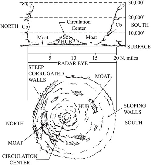
FIGURE 1. Schematic diagram of the eye of Hurricane Edna, 9–10 September 1954, as adapted from Simpson and Starrett (1955). At this time, Hurricane Edna had a steep corrugated eyewall on its north side and a sloping $(\approx 45°)$ eyewall on its south side. Such variations in eyewall slope are often interpreted as an effect of environmental vertical shear (see Hazelton and Hart, 2013; Hazelton et al., 2015; and the recent review by Rogers, 2021). The stratocumulus “hub cloud” near the circulation center and the moat near the edge of the eye indicate that in strong hurricanes the subsidence is not uniform across the eye, but rather is concentrated near the edge of the eye. Enhanced subsidence in the lower troposphere near the edge of the eye leads to a lower-tropospheric warm-ring thermal structure, as shown in Figure 2 for Hurricane Isabel (2003). A photograph of Isabel’s hub cloud is shown in Figure 3, which indicates that the hub clouds in Isabel and Edna were of approximately the same height, although Isabel’s eye diameter was somewhat larger than that of Edna.

FIGURE 2

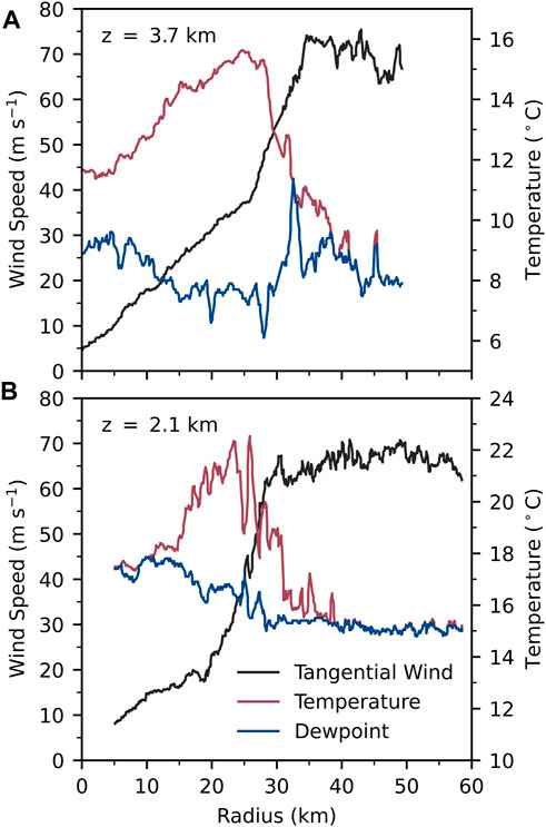
FIGURE 2. Radial profiles of NOAA WP-3D aircraft data for Hurricane Isabel on 13 September 2003. The panel (B) is for the z = 2.1 km flight leg (1922 to 1931 UTC) and the panel (A) for the z = 3.7 km flight leg (1948 to 1956 UTC). Black curves are for tangential wind, red curves for temperature, and blue curves for dewpoint temperature. Adapted from Schubert et al. (2007).

The photograph shown here as Figure 3 was taken from the WP-3D aircraft near the edge of the eye, looking towards the hub cloud at the center of the eye. The top of the hub cloud is near 3 km altitude, so the radial leg in the upper panel of Figure 2 is just above the top of the hub cloud, while the radial leg in the lower panel is just below the top of the hub cloud, as is evident in the dewpoint depressions. Since the first internal mode Rossby length in the eye of Isabel at this time is on the order of 10–15 km, the eye diameter ($\sim 60$ km) is approximately 5 Rossby lengths, allowing for the rare opportunity to view balanced dynamical structure over several Rossby lengths in a single photograph. For comprehensive discussions of Hurricane Isabel, see Montgomery et al. (2006), Aberson et al. (2006), Bell and Montgomery (2008), Nolan et al. (2009b,a), and Stern et al. (2016). The eye-moat and mesovortex structure of Hurricane Isabel on 12 September 2003 is discussed by Kossin and Schubert (2004) and Rozoff et al. (2006).

FIGURE 3

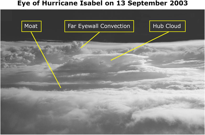
FIGURE 3. Photograph of the eye of Hurricane Isabel on 13 September 2003. The 3 km tall hub cloud at the center of the eye is surrounded by a moat of clear air or shallow stratocumulus. Beyond the hub cloud and on the opposite side of the eye (at a distance of $\sim 60$ km) lies eyewall convection extending up to 12–14 km. Photo courtesy of Sim Aberson.

Another common feature of intense tropical cyclones is the “stadium effect,” caused by the outward slope of the eyewall. An example of this effect, taken from the CloudSat data archive, is shown in Figure 4. This vertical cross-section was obtained when CloudSat’s 94 GHz Cloud Profiling Radar made a fortuitous pass directly over the eye of Typhoon Choi-Wan on 15 September 2009. In the top panel of Figure 4, the vertical scale is stretched to highlight the vertical structure of the radar reflectivity. In the bottom panel, only the region inside a radius of 50 km is shown, so the aspect ratio is one-to-one, which clearly reveals the approximate 45° baroclinic tilt of the eyewall updraft. The incorporation of such baroclinic tilt is an important aspect of the theoretical analysis presented here in Sections 2 and 3.

FIGURE 4

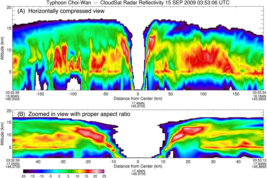
FIGURE 4. At 0353 UTC on 15 September 2009, CloudSat’s 94 GHz Cloud Profiling Radar passed directly over Typhoon Choi-Wan. This figure shows a north-south vertical cross-section of radar reflectivity for the 65 m s⁻¹ storm (north is to the right) when it was located approximately 450 km north of Guam. In the panel (A), the horizontal scale is compressed to exaggerate the vertical structure. In the panel (B), only the region inside a radius of 50 km is shown (which excludes the secondary eyewall), but the aspect ratio is one-to-one, thus showing the sloping eyewall (or “stadium effect”) as would be seen by an observer on a research aircraft. Reflectivity values less than − 20 dBZ have been removed for clarity. This figure has been adapted from Schubert and McNoldy (2010) and is based on radar data made available through the NASA CloudSat Project.

An interesting feature of nonhydrostatic, full-physics, tropical cyclone models is that they can produce intense storms with a temperature field that has a warm-core structure at upper levels, but a warm-ring structure at lower levels. The first example of this was presented by Yamasaki (1983), whose Figure 10A is reproduced here as Figure 5. The upper tropospheric warm-core anomaly is 17°C and is centered at a height of 14 km. A warm-ring thermal structure is found between heights of 2 and 8 km, and at a radius of approximately 7–8 km. Much of the present paper is devoted to a balanced dynamical interpretation of the production of such an overall thermal structure.

FIGURE 5

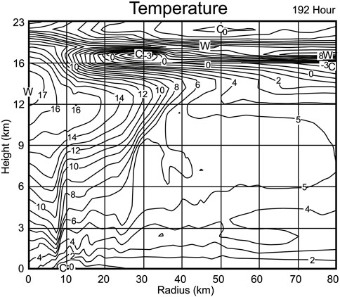
FIGURE 5. Vertical cross-section of the temperature anomaly (°C) from the nonhydrostatic, full-physics model simulation of an intense tropical cyclone by Yamasaki (1983). A warm-core thermal structure (17°C anomaly) is found at heights near 14 km, while a warm-ring thermal structure is found near r ≈ 7–8 km between heights of 2 and 8 km. As shown in Eq. 35 the warm-ring thermal structure is associated with absolute angular momentum surfaces that are tilted in opposite directions on the two sides of the warm ring. The upper troposphere/lower stratosphere cold anomaly produced by this model is similar to that observed by Johnson and Kriete (1982) for tropical mesoscale systems using radiosonde data (their Figure 3) and by Rivoire et al. (2016) using COSMIC GPS radio occultation data. Adapted from Figure 10A of Yamasaki (1983).

For the study of eye subsidence, one can envision using (at least) four different sets of independent variables in space: radius and log-pressure, (r, z); potential radius and log-pressure, (R, Z); radius and potential temperature, (r, θ); or potential radius and potential temperature, (R, Θ). Note that Z = z and Θ = θ, but the upper case symbols Z and Θ are used because (∂/∂Z) ≠ (∂/∂z) and (∂/∂Θ) ≠ (∂/∂θ). Concerning the use of (R, Θ)-coordinates, since the flow in the eye is inviscid and adiabatic, both R and Θ are Lagrangian coordinates, which means that a given parcel in the eye stays on its original R-surface and its original Θ-surface. In other words, when the mathematical analysis is performed in (R, Θ)-space, there is no need for a transverse circulation equation, and the dynamics is more easily understood in the framework of PV and its invertibility principle, as discussed in a theoretical context by Schubert and Alworth (1987), Möller and Smith (1994), and Schubert (2018), and in an observational context by Martinez et al. (2019). This is in sharp contrast to the use of (r, z)-coordinates, where neither r nor z is a Lagrangian coordinate. In this paper, we have analyzed the transverse circulation problem in (R, Z)-coordinates, a setting in which one coordinate is Lagrangian and the other is not. There is a duality between the use of (R, Z)-coordinates and the use of (r, θ)-coordinates, since in the (r, θ)-formulation, one coordinate is Lagrangian (recall that $\dot{\theta }=0$ in the eye) and the other is not. Thus, the essential results obtained in Section 3 using the (R, Z)-formulation could also be obtained using the (r, θ)-formulation. However, some details involved in the two formulations are different. For example, in the (r, θ)-formulation, a convenient vertically sheared Rankine core has solid-body rotation on each isentropic surface rather than on each isobaric surface. Also, in the elliptic problem (Eq. 16), the outer boundary is the coordinate surface R = R_ew, while in the (r, θ)-formulation a sloping eyewall outer boundary would not be an r-surface, thereby producing an additional difficulty in the solution of the elliptic problem. Thus, while the difficulties of including baroclinic effects in the (r, z)-formulation can be overcome by using either the (R, Z)-formulation or the (r, θ)-formulation, the analysis presented in this paper is indicative of our slight preference for the (R, Z)-formulation.

The paper is organized as follows. Section 2 first presents the balanced vortex equations in the (r, z)-formulation, and then transforms to the (R, Z)-formulation. For certain baroclinic vortices, the (R, Z) formulation of the transverse circulation equation can be solved semi-analytically using a vertical transform approach (Section 3). These semi-analytical solutions are used to generalize the barotropic vortex results of Schubert et al. (2007) and to better understand the role of baroclinicity in the distribution of subsidence in the eye of an intense tropical cyclone.

2 Gradient balance theory

For simplicity, the analysis presented here considers an axisymmetric, balanced flow in the inviscid fluid that lies above the frictional boundary layer. To simplify the primitive equation model to a balanced vortex model, we assume that the azimuthal flow remains in a gradient balanced state, i.e., we discard the exact radial equation of motion and replace it with the gradient balance condition given below as the first entry in Eq. 1. A sufficient condition for the validity of this assumption is that the diabatic forcing effects have slow enough time scales that significant, azimuthal mean inertia-gravity waves are not excited. We shall describe this inviscid flow using the log-pressure vertical coordinate z = H ln(p₀/p), where H = R_dT₀/g is the constant scale height, p₀ and T₀ are constant reference values of pressure and temperature, R_d is the gas constant for dry air, and g is the acceleration of gravity. Under the balance condition, the governing equations are

$\begin{array}{ll}\hfill \left(f+\frac{v}{r}\right)& v=\frac{\partial \varphi }{\partial r},\hfill \\ \hfill \frac{\partial v}{\partial t}+w\frac{\partial v}{\partial z}& +\left(f+\frac{\partial \left(rv\right)}{r\partial r}\right)u=0,\hfill \\ \hfill \frac{\partial \varphi }{\partial z}& =\frac{g}{T_0}T,\hfill \\ \hfill \frac{\partial \left(ru\right)}{r\partial r}& +\frac{\partial \left(\rho w\right)}{\rho \partial z}=0,\hfill \\ \hfill \frac{\partial T}{\partial t}+u\frac{\partial T}{\partial r}& +w\left(\frac{\partial T}{\partial z}+\frac{\kappa T}{H}\right)=\frac{Q}{c_{\text{p}}},\hfill \end{array}(1)$

where κ = R_d/c_p, c_p is the specific heat at constant pressure, f the constant Coriolis parameter, ρ(z) = ρ₀e^−z/H the pseudo-density in the log-pressure coordinate, ρ₀ = p₀/(R_dT₀) the constant reference density, ϕ the geopotential, u the radial velocity component, v the azimuthal velocity component, w the log-pressure vertical velocity, and Q the diabatic heating. The potential vorticity (PV) equation, derived from Eq. 1, is

$\frac{DP}{Dt}=\frac{1}{\rho }\left[-\frac{\partial v}{\partial z}\frac{\partial \dot{\theta }}{\partial r}+\left(f+\frac{\partial \left(rv\right)}{r\partial r}\right)\frac{\partial \dot{\theta }}{\partial z}\right],(2)$

where D/Dt = (∂/∂t) + u(∂/∂r) + w(∂/∂z) is the material derivative,

$P=\frac{1}{\rho }\left[-\frac{\partial v}{\partial z}\frac{\partial \theta }{\partial r}+\left(f+\frac{\partial \left(rv\right)}{r\partial r}\right)\frac{\partial \theta }{\partial z}\right]=\frac{fR}{\rho r}\frac{\partial \left(R,\theta \right)}{\partial \left(r,z\right)}(3)$

is the potential vorticity, $\theta =T{(p_0/p)}^{\kappa }=T{e}^{\kappa z/H}$ is the potential temperature, $c_{\text{p}}\dot{\theta }/\theta =Q/T$, and the potential radius R is defined in terms of the absolute angular momentum by $\frac{1}{2}f{R}^2=rv+\frac{1}{2}f{r}^2$.

Using the mass conservation principle, we define a streamfunction ψ such that

$\rho u=-\frac{\partial \psi }{\partial z}\text{and}\rho w=\frac{\partial \left(r\psi \right)}{r\partial r}.(4)$

For convenience, we shall refer to ψ as the “streamfunction,” although it is worth noting that it is actually rψ, rather than ψ, that is the “streamfunction” for the transverse mass flux. This flexibility with the factor r proves convenient for the analytical solutions presented in Section 3. Using the gradient balance relation in the tangential wind equation, and using the hydrostatic relation in the thermodynamic equation, we can write

$\begin{array}{ll}\hfill \frac{\partial {\varphi }_t}{\partial r}-\rho Bw+\rho Cu& =0,\hfill \\ \hfill \frac{\partial {\varphi }_t}{\partial z}+\rho Aw-\rho Bu& =\frac{gQ}{c_{\text{p}}{T}_0},\hfill \end{array}(5)$

where ϕ_t = (∂ϕ/∂t) is the geopotential tendency, and where the static stability A, the baroclinicity B, and the inertial stability C are given by

$\begin{array}{ll}\hfill \rho A& =\frac{g}{T_0}\left(\frac{\partial T}{\partial z}+\frac{\kappa T}{H}\right),\hfill \\ \hfill \rho B& =-\left(f+\frac{2v}{r}\right)\frac{\partial v}{\partial z}=-\frac{g}{T_0}\frac{\partial T}{\partial r},\hfill \\ \hfill \rho C& =\left(f+\frac{2v}{r}\right)\left(f+\frac{\partial \left(rv\right)}{r\partial r}\right).\hfill \end{array}(6)$

Eliminating ϕ_t between the two equations in Eq. 5, then expressing u and w in terms of ψ via Eq. 4, and requiring that w = 0 at the top and bottom boundaries, we obtain the following transverse circulation problem (Eliassen, 1951).

$\begin{array}{cc}\hfill & \mathbf{\text{Secondary Circulation Problem on the Full}}\left(\mathit{r},\mathit{z}\right)-\mathbf{Domain:}\hfill \\ \hfill & \frac{\partial }{\partial r}\left(A\frac{\partial \left(r\psi \right)}{r\partial r}+B\frac{\partial \psi }{\partial z}\right)+\frac{\partial }{\partial z}\left(B\frac{\partial \left(r\psi \right)}{r\partial r}+C\frac{\partial \psi }{\partial z}\right)=\frac{g}{c_{\text{p}}{T}_0}\frac{\partial Q}{\partial r}\text{for}0\le r<\infty \text{and}0\le z\le z_{\text{T}}\text{with}\left\{\begin{array}{c}\psi \left(0,z\right)=\psi \left(r,0\right)=\psi \left(r,z_{\text{T}}\right)=0,\hfill \\ r\psi \left(r,z\right)\to 0\text{as}r\to \infty .\hfill \end{array}\right.\hfill \end{array}(7)$

Note that $AC-B^2=g{T}_0^{-1}{\rho }_0^{-1}{e}^{(1-\kappa )z/H}\left(f+2v/r\right)P$, so that this problem is elliptic if (f + 2v/r)P > 0, which is typically the case for the tropical cyclone core region studied in this paper.

According to Eq. 7, subsidence in the hurricane eye at a particular time is forced by the (∂Q/∂r) term and is shaped by the three spatially varying coefficients A, B, C at that time. Analytical progress in understanding eye subsidence can more easily be made if we obtain a transformed version of Eq. 7 that contains only two spatially varying coefficients and does not contain any second order mixed derivative terms. The balanced vortex model and the associated transverse circulation equation take simple forms when the original independent variables (r, z, t) are replaced by the new independent variables (R, Z, τ), where Z = z and τ = t but ∂/∂Z and ∂/∂τ imply fixed potential radius R. This transformation (Schubert and Hack, 1983) makes use of

$\left(\frac{\partial }{\partial r},\frac{\partial }{\partial z},\frac{\partial }{\partial t}\right)=\left(\frac{\partial R}{\partial r}\frac{\partial }{\partial R},\frac{\partial R}{\partial z}\frac{\partial }{\partial R}+\frac{\partial }{\partial Z},\frac{\partial R}{\partial t}\frac{\partial }{\partial R}+\frac{\partial }{\partial \tau }\right),(8)$

from which it follows that

$\frac{D}{Dt}=\frac{\partial }{\partial t}+u\frac{\partial }{\partial r}+w\frac{\partial }{\partial z}=\frac{\partial }{\partial \tau }+w\frac{\partial }{\partial Z}.(9)$

Defining U, V, W, and Φ by

$\begin{array}{cc}\hfill U& =\frac{r}{R}u+\frac{w}{f}\frac{\partial V}{\partial Z},\hfill \\ \hfill V& =\frac{r}{R}v,\hfill \end{array}\begin{array}{cc}\hfill W& =\left(\frac{f}{f+\zeta }\right)w,\hfill \\ \hfill \mathrm{\Phi }& =\varphi +\frac{1}{2}{v}^2,\hfill \end{array}(10)$

where ζ = r⁻¹∂(rv)/∂r is the relative vorticity, the governing equations (Eq. 1) transform to (see Appendix A for further details)

$\begin{array}{cc}\hfill & \widehat{f}V=\frac{\partial \mathrm{\Phi }}{\partial R},\hfill \\ \hfill & \frac{\partial V}{\partial \tau }+fU=0,\hfill \\ \hfill & \frac{\partial \mathrm{\Phi }}{\partial Z}=\frac{g}{T_0}T,\hfill \end{array}\begin{array}{cc}\hfill & \frac{\partial \left(RU\right)}{R\partial R}+\frac{\partial \left(\rho W\right)}{\rho \partial Z}=0,\frac{\partial T}{\partial \tau }+\frac{T_0}{g}{N}^{2}W=\frac{Q}{c_{\text{p}}},\hfill \end{array}(11)$

where the effective inertial frequency $\widehat{f}$ and the effective buoyancy frequency N are defined by

$\begin{array}{ll}\hfill {\widehat{f}}^2& ={\left(f+\frac{2v}{r}\right)}^2=f^2\frac{R^4}{r^4}=f^4{\left(f-\frac{2V}{R}\right)}^{-2},\hfill \\ \hfill N^2& =\left(\frac{f+\zeta }{f}\right)\frac{g}{T_0}\left(\frac{\partial T}{\partial Z}+\frac{\kappa T}{H}\right)\hfill \\ \hfill & =e^{-\kappa Z/H}\left(\frac{f+\zeta }{f}\right)\frac{g}{T_0}\frac{\partial \theta }{\partial Z}=e^{-\kappa Z/H}\frac{g\rho P}{T_{0}f}.\hfill \end{array}(12)$

It follows that r and R are related by $r={(f/\widehat{f})}^{1/2}R$ and that rv = RV. Note that the system in Eq. 11 is formally simpler than the system in Eq. 1, even though no additional approximations have been introduced. Also note that the effective buoyancy frequency N can differ greatly from the usual buoyancy frequency in the cyclone core, but they are essentially the same in far-field regions where |ζ| ≪ f and the angular momentum surfaces are nearly vertical, so that (∂T/∂Z) ≈ (∂T/∂z) and (∂θ/∂Z) ≈ (∂θ/∂z).

Using the fourth entry in Eq. 11, we define the streamfunction Ψ such that

$\rho U=-\frac{\partial \mathrm{\Psi }}{\partial Z}\text{and}\rho W=\frac{\partial \left(R\mathrm{\Psi }\right)}{R\partial R}.(13)$

From Eqs. 4 and 13, and the transformation relations in Eq. 8, it can be shown that RΨ and rψ differ only by a constant, which, without loss of generality, we can take to be zero, so that RΨ = rψ. Using the gradient balance relation in the tangential wind equation, and using the hydrostatic relation in the thermodynamic equation, we can write

$\frac{\partial {\mathrm{\Phi }}_{\tau }}{\partial R}+{\widehat{f}}^{2}U=0\text{and}\frac{\partial {\mathrm{\Phi }}_{\tau }}{\partial Z}+N^{2}W=\frac{gQ}{c_{\text{p}}{T}_0},(14)$

where Φ_τ = (∂Φ/∂τ) = (∂ϕ/∂t) is the “geopotential tendency.” Eliminating Φ_τ between these two equations, and then expressing U and W in terms of Ψ via Eq. 13, we obtain the following transverse circulation problem.

$\begin{array}{cc}\hfill & \mathbf{\text{Secondary Circulation Problem on the Full}}\left(\mathit{R},\mathit{Z}\right)-\mathbf{\text{Domain:}}\hfill \\ \hfill & \frac{\partial }{\partial R}\left(N^2{e}^{Z/H}\frac{\partial \left(R\mathrm{\Psi }\right)}{R\partial R}\right)+\frac{\partial }{\partial Z}\left({\widehat{f}}^2{e}^{Z/H}\frac{\partial \mathrm{\Psi }}{\partial Z}\right)=\frac{g{\rho }_0}{c_{\text{p}}{T}_0}\frac{\partial Q}{\partial R}\hfill \\ \text{for}0\le R<\infty \text{and}0\le Z\le Z_{\text{T}}\text{with}\left\{\begin{array}{c}\mathrm{\Psi }\left(0,Z\right)=\mathrm{\Psi }\left(R,0\right)=\mathrm{\Psi }\left(R,Z_{\text{T}}\right)=0,\hfill \\ R\mathrm{\Psi }\left(R,Z\right)\to 0\text{as}R\to \infty .\hfill \end{array}\right.\hfill \end{array}(15)$

The boundary conditions on Ψ come from the requirement that the log-pressure vertical velocity vanishes at the bottom and top boundaries, that the radial component of the secondary circulation vanishes at R = 0, and that the secondary circulation goes to zero as R → ∞. To summarize, the secondary circulation in the entire region is obtained by solving the elliptic problem in Eq. 15 for specified N(R, Z), $\widehat{f}(R,Z)$, and Q(R, Z). Note that Eq. 15 is formally simpler than Eq. 7 since it does not contain baroclinic, second order cross derivative terms. Baroclinic effects are implicit in Eq. 15 and are recovered when the solution Ψ(R, Z) is transformed back to the physical space form ψ(r, z) using ψ = (R/r)Ψ.

We can understand several aspects of eye subsidence by solution of a restricted version of the full elliptic problem in Eq. 15. In this simplified problem, we restrict our attention to the eye region 0 ≤ R ≤ R_ew, where the eyewall potential radius R_ew (i.e., the inner edge of the eyewall) is assumed to be a constant. In the eye region, we assume that Q = 0, so that the elliptic problem in Eq. 15 simplifies as follows.

$\begin{array}{cc}\hfill & \mathbf{\text{Secondary Circulation Problem on the Restricted}}\left(\mathit{R},\mathit{Z}\right)-\mathbf{\text{Domain:}}\hfill \\ \hfill & \frac{\partial }{\partial R}\left(N^2{e}^{Z/H}\frac{\partial \left(R\mathrm{\Psi }\right)}{R\partial R}\right)+\frac{\partial }{\partial Z}\left({\widehat{f}}^2{e}^{Z/H}\frac{\partial \mathrm{\Psi }}{\partial Z}\right)=0\hfill \\ \hfill & \text{for}0\le R\le R_{\text{ew}}\text{and}0\le Z\le Z_{\text{T}}\text{with}\hfill \\ \hfill & \left\{\begin{array}{c}\mathrm{\Psi }\left(0,Z\right)=\mathrm{\Psi }\left(R,0\right)=\mathrm{\Psi }\left(R,Z_{\text{T}}\right)=0,\hfill \\ \mathrm{\Psi }\left(R_{\text{ew}},Z\right)={\mathrm{\Psi }}_{\text{ew}}\left(Z\right).\hfill \end{array}\right.\hfill \end{array}(16)$

To summarize, the secondary circulation in the eye is obtained by solving the homogeneous, elliptic problem in Eq. 16 with specified N(R, Z), $\widehat{f}(R,Z)$, and Ψ_ew(Z). Note that all the dynamics in the region R_ew < R < ∞, described explicitly in Eq. 15, has been replaced in Eq. 16 by the specification of Ψ(R, Z) at R = R_ew. Because the elliptic problem in Eq. 16 is homogeneous, the solution Ψ(R, Z) has no local maxima or minima in the interior of the restricted domain (i.e., in the eye). For the problems considered here, we have chosen Ψ_ew(Z) ≤ 0, so that Ψ(R, Z) attains its minimum value on the outer boundary R = R_ew and its maximum value of zero on the other three boundaries, R = 0 and Z = 0, Z_T, where Z_T = z_T represents the tropopause. By concentrating attention on the restricted problem (Eq. 16), the goal is to understand how the spatial structure of eye subsidence is shaped by N(R, Z), $\widehat{f}(R,Z)$, and Ψ_ew(Z). A semi-analytical solution of a simplified version of Eq. 16 is given in Section 3, using vertical transform methods. An alternative approach, not explored here, is to study solutions of the geopotential tendency equation (see Appendix B).

3 Subsidence in a vertically sheared, Rankine vortex core

3.1 The specified vortex

We now solve Eq. 16 semi-analytically for particular choices of the coefficients $\widehat{f}(R,Z)$ and N(R, Z). For the example given here, the vortex core is assumed to have constant angular velocity (i.e., solid body rotation) on each isobaric surface, but with the angular velocity varying in the vertical. In terms of v(r, z) and θ(r, z), the specified vortex for 0 ≤ r ≤ r_ew(z) and 0 ≤ z ≤ z_T is given by

$\left\{\begin{array}{cc}v\left(r,z\right)\hfill & =\frac{1}{2}\left(\widehat{f}\left(z\right)-f\right)r,\hfill \\ \widehat{f}\left(z\right)\hfill & ={\widehat{f}}_{\text{T}}+\left({\widehat{f}}_0-{\widehat{f}}_{\text{T}}\right)\left(\frac{e^{-\kappa z/H}-e^{-\kappa z_{\text{T}}/H}}{1-e^{-\kappa z_{\text{T}}/H}}\right),\hfill \\ \hfill \theta \left(r,z\right)& ={\theta }_{\text{c}}\left(z\right)-\frac{\left({\widehat{f}}_0-{\widehat{f}}_{\text{T}}\right)\widehat{f}\left(z\right)r^2}{4c_{\text{p}}\left(1-e^{-\kappa z_{\text{T}}/H}\right)},\hfill \end{array}\right.(17)$

where, for this vertically sheared Rankine core, the effective inertial frequency $\widehat{f}(z)$ is also the absolute vorticity in the eye, the constants ${\widehat{f}}_0$ and ${\widehat{f}}_{\text{T}}$ are the specified values of $\widehat{f}(z)$ at z = 0 and z = z_T respectively, and $r_{\text{ew}}(z)={[f/\widehat{f}(z)]}^{1/2}{R}_{\text{ew}}$, with the constant R_ew denoting the potential radius of the inner edge of the eyewall. The specified function θ_c(z) is the potential temperature at the vortex center, which is simply taken as a quadratic function of z varying from 300 K at z = 0 to 370 K at z = z_T = 16 km, i.e.,

${\theta }_{\text{c}}\left(z\right)=300\mathrm{K}+\frac{z}{z_{\text{T}}}\left[70\mathrm{K}+52\mathrm{K}\left(1-\frac{z}{z_{\text{T}}}\right)\right].(18)$

This profile, shown by the dashed blue line in Figure 6, has been constructed to approximate the θ-profile for the center of Hurricane Hilda, as described by Hawkins and Rubsam (1968) and shown by the solid blue curve in Figure 6. For reference, the mean profiles for the West Indies, as given by Jordan (1958), and the mean profiles for the Marshall Islands and GATE, as given by Fulton and Schubert (1985), are shown by the other colored curves, thereby illustrating the warming of the core of Hilda relative to a far-field environment. In addition to this profile, we have chosen the following parameters for our analyses of both the barotropic and baroclinic cases: R_d = 287 J kg⁻¹ K⁻¹, T₀ = 300 K, p₀ = 1000 hPa, g = 9.81 m s⁻², H = R_dT₀/g = 8,777 m, f = 5 × 10^–5 s⁻¹, and z_T = 16 km.

FIGURE 6

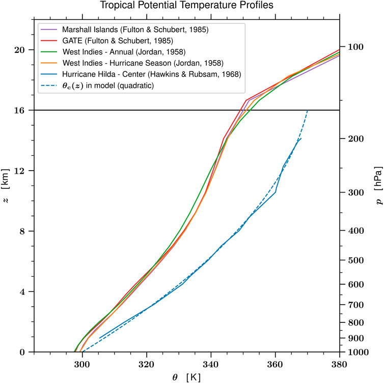
FIGURE 6. The solid blue curve is the θ profile in the core of Hurricane Hilda, as described by Hawkins and Rubsam (1968). The dashed blue curve is the quadratic approximation θ_c(z) given by Eq. 18. For reference, the annual mean and hurricane season mean profiles for the West Indies (Jordan, 1958) and the mean profiles for the Marshall Islands and GATE (Fulton and Schubert, 1985) are shown by the other colored curves. The maximum warm-core anomaly in θ occurs at 300 hPa and is approximately 21 K. The horizontal line at z = 16 km denotes the upper boundary used in the calculations presented in Section 3.

As is easily confirmed, the v(r, z) and θ(r, z) fields given in Eq. 17 satisfy the thermal wind relation $\widehat{f}(\partial v/\partial z)=(g/T_0)(\partial \theta /\partial r)e^{-\kappa z/H}$. The choice ${\widehat{f}}_0={\widehat{f}}_{\text{T}}$ corresponds to a barotropic vortex, which is the case studied by Schubert et al. (2007). The vortex specified in Eq. 17 is plotted in the left panel of Figure 7 for the barotropic case ${\widehat{f}}_0={\widehat{f}}_{\text{T}}=64f$ and R_ew = 240 km, so that r_ew(z) = 30 km and v(r_ew(z), z) = 47.3 m s⁻¹. For barotropic cases such as the one shown in Figure 7A, the isolines of v and R are vertical, while the isentropes are parallel to the isobars. The right panel of Figure 7 is for the baroclinic case ${\widehat{f}}_0=144f$, ${\widehat{f}}_{\text{T}}=36f$, and R_ew = 240 km, so that $\frac{1}{2}f{R}_{\text{ew}}=6$ m s⁻¹, r_ew(0) = 20 km, r_ew(z_T) = 40 km, v(r_ew(0), 0) = 71.5 m s⁻¹, and v(r_ew(z_T), z_T) = 35 m s⁻¹. Note that this baroclinic vortex is warm-core at all levels, with the highest values of θ on any isobaric surface occurring at r = 0 and with outward-tilting R-surfaces. The maximum values of v(r, z) occur on the R_ew = 240 km surface, which is consistent with the observation (Stern and Nolan, 2009) that, for the majority of storms, the radius of maximum wind is closely approximated by an R-surface.

FIGURE 7

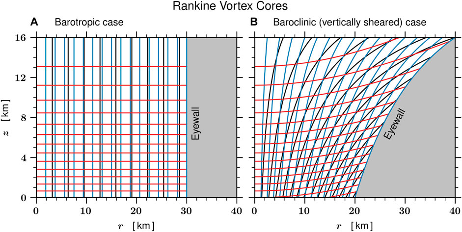
FIGURE 7. Structure of the Rankine vortex core, as described by Eq. 17, for both the barotropic case (A) where ${\widehat{f}}_0={\widehat{f}}_{\text{T}}=64f$ and the baroclinic (vertically sheared) case (B) where ${\widehat{f}}_0=144f$ and ${\widehat{f}}_{\text{T}}=36f$. The three sets of contours (black, blue, and red) are for v(r, z), R(r, z) and θ(r, z) in the eye region, which is bounded by an eyewall at R = R_ew = 240 km. The physical radius for the eyewall, given by $r_{\text{ew}}(z)={[f/\widehat{f}(z)]}^{1/2}{R}_{\text{ew}}$, has a constant value of 30 km in the barotropic case but slopes outward between r = 20 km and r = 40 km in the baroclinic case. In panel (A), the black contours for v(r, z) run from 5 to 45 m s⁻¹ in increments of 5 m s⁻¹, the blue contours for R(r, z) run from 15 to 240 km in increments of 15 km, while the red contours for θ(r, z) run from 305 K to 365 K in increments of 5 K. In panel (B), the black contours for v(r, z) run from 5 to 70 m s⁻¹ in increments of 5 m s⁻¹, the blue contours for R(r, z) run from 15 to 240 km in increments of 15 km, while the red contours for θ(r, z) run from 295 K to 365 K in increments of 5 K.

Written in terms of V(R, Z) and θ(R, Z), the specified vortex in Eq. 17 for 0 ≤ R ≤ R_ew and 0 ≤ Z ≤ Z_T is given by

$\left\{\begin{array}{cc}\hfill V\left(R,Z\right)& =\frac{1}{2}f\left(\frac{\widehat{f}\left(Z\right)-f}{\widehat{f}\left(Z\right)}\right)R,\hfill \\ \widehat{f}\left(Z\right)\hfill & ={\widehat{f}}_{\text{T}}+\left({\widehat{f}}_0-{\widehat{f}}_{\text{T}}\right)\left(\frac{e^{-\kappa Z/H}-e^{-\kappa Z_{\text{T}}/H}}{1-e^{-\kappa Z_{\text{T}}/H}}\right),\hfill \\ \hfill \theta \left(R,Z\right)& ={\theta }_{\text{c}}\left(Z\right)-\frac{\left({\widehat{f}}_0-{\widehat{f}}_{\text{T}}\right)f{R}^2}{4c_{\text{p}}\left(1-e^{-\kappa Z_{\text{T}}/H}\right)}.\hfill \end{array}\right.(19)$

As is also easily confirmed, the V(R, Z) and θ(R, Z) fields given in Eq. 19 satisfy the thermal wind relation $({\widehat{f}}^2/f)(\partial V/\partial Z)=(g/T_0)(\partial \theta /\partial R)e^{-\kappa Z/H}$. A crucial property of this vertically sheared Rankine-like vortex core is that the θ(R, Z) field, given by the last line in Eq. 19, is the sum of a function of Z and a function of R. Using the last line of Eq. 19, we find that N² and P take the simplified forms

$\begin{array}{ll}\hfill N^2\left(z\right)& =e^{-\kappa z/H}\frac{\widehat{f}\left(z\right)}{f}\frac{g}{T_0}\frac{d{\theta }_{\text{c}}\left(z\right)}{dz},\hfill \\ \hfill P\left(z\right)& =\frac{1}{\rho \left(z\right)}\widehat{f}\left(z\right)\frac{d{\theta }_{\text{c}}\left(z\right)}{dz},\hfill \end{array}(20)$

so that both N² and P are functions of z only for the vertically sheared Rankine core. This allows the solution of Eq. 16 to be written in separable form, i.e., it allows for the analytical solution of Eq. 16 using the vertical normal mode transform method discussed below. The shape of the secondary circulation in the eye depends on the outward tilt of the R = R_ew absolute angular momentum surface and on the ratio of the two variable coefficients in Eq. 16. It is convenient to multiply this ratio by the constant scale height H to obtain the local Rossby length $[N(Z)/\widehat{f}(Z)]H\sim {[\widehat{f}(Z)]}^{-1/2}$, so that in the typical situation for which $\widehat{f}$ decreases with height, the local Rossby length is smallest in the lower troposphere. This leads to the expectation that the compensating subsidence in the eye occurs closer to the eyewall in the lower troposphere than in the upper troposphere. An alternative interpretation of the dynamics involves the definition of Rossby length via vertical mode rather than locally. This alternative interpretation is given in the discussion of the results shown in Table 1.

TABLE 1

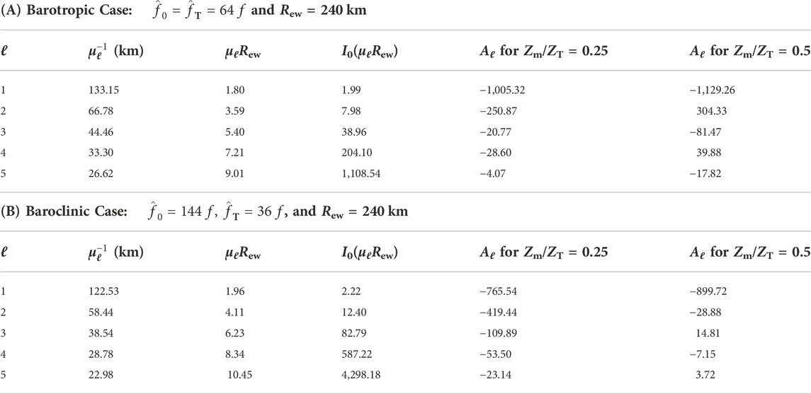
TABLE 1. Numerical results for the barotropic case (top table) and the baroclinic case (bottom table). The first column lists the vertical mode index ℓ, while the second column lists the corresponding values of the Rossby length ${\mu }_{\ell }^{-1}$, which are determined from the eigenvalues of the Sturm–Liouville problem in Eq. 23. Note that the crude approximation ${\mu }_{\ell }^{-1}\approx {\mu }_1^{-1}/\ell$, which can be derived for the special case where N² and $\widehat{f}$ are constants, works better for the barotropic case, for which $\widehat{f}(z)$ is a constant. The five corresponding eigenfunctions are shown in the left and right panels of Figure 8. For the choice R_ew = 240 km, the third column lists values of μ_ℓR_ew, which can be interpreted as the number of Rossby lengths (in R-space) between the vortex center R = 0 and the inner edge of the eyewall R = R_ew. The fourth column lists values of I₀(μ_ℓR_ew), which can be interpreted as the factor by which (for given ℓ) the subsidence at the center is reduced from that at the edge of the eye. The large value of I₀(μ_ℓR_ew) for ℓ ≥ 2 indicate the importance of the higher vertical modes in producing a lower-tropospheric warm-ring structure. Columns 5 and 6 tabulate the projection of Ψ_ew(Z) onto the first five vertical modes, as computed from Eq. 29.

3.2 Solution via the vertical transform method

For the vertically sheared Rankine vortex core, the restricted problem given in Eq. 16 simplifies considerably because N and $\widehat{f}$ are functions of Z only. Then, the elliptic partial differential equation reduces to

$\frac{{\partial }^2\mathrm{\Psi }}{\partial R^2}+\frac{\partial \mathrm{\Psi }}{R\partial R}-\frac{\mathrm{\Psi }}{R^2}+\frac{e^{-Z/H}}{N^2}\frac{\partial }{\partial Z}\left({\widehat{f}}^2{e}^{Z/H}\frac{\partial \mathrm{\Psi }}{\partial Z}\right)=0.(21)$

We now solve Eq. 21 using the vertical transform method. The vertical transform pair is

$\begin{array}{ll}\hfill \mathrm{\Psi }\left(R,Z\right)& =\sum _{\ell =1}^{\infty }{\mathrm{\Psi }}_{\ell }\left(R\right){\mathcal{Z}}_{\ell }\left(Z\right),\hfill \\ \hfill {\mathrm{\Psi }}_{\ell }\left(R\right)& =\frac{1}{N_0^{2}H}{\int }_0^{Z_{\text{T}}}\mathrm{\Psi }\left(R,Z\right){\mathcal{Z}}_{\ell }\left(Z\right)N^2\left(Z\right)e^{Z/H}dZ,\hfill \end{array}(22)$

where the kernel ${\mathcal{Z}}_{\ell }(Z)$ of the transform is defined to be the solution of

$\begin{array}{ll}\hfill & \frac{e^{-Z/H}}{N^2}\frac{d}{dZ}\left({\widehat{f}}^2{e}^{Z/H}\frac{d{\mathcal{Z}}_{\ell }}{dZ}\right)+{\mu }_{\ell }^2{\mathcal{Z}}_{\ell }=0\text{with}{\mathcal{Z}}_{\ell }\left(0\right)={\mathcal{Z}}_{\ell }\left(Z_{\text{T}}\right)=0,\hfill \end{array}(23)$

which is a second order differential problem of the Sturm–Liouville type (e.g., Arfken and Weber, 2005, Chapter 10). In this method of solution, the streamfunction Ψ(R, Z) is represented as an infinite series of eigenfunctions ${\mathcal{Z}}_{\ell }(Z)$ with corresponding eigenvalues μ_ℓ. The constant surface value of the effective buoyancy frequency, denoted by N₀, has been introduced into the weight function $[N^2(Z)/N_0^2][e^{Z/H}/H]$ so that, if ${\mathcal{Z}}_{\ell }(Z)$ is normalized in such a way that it is dimensionless, then Ψ(R, Z) and Ψ_ℓ(R) will have the same units. The orthonormality of the vertical structure functions ${\mathcal{Z}}_{\ell }(Z)$ is discussed in Appendix C, as is the derivation of the second entry in Eq. 22 using this orthonormality relation.

To take the vertical transform of Eq. 21, first multiply it by ${\mathcal{Z}}_{\ell }(Z)[N^2(Z)/N_0^2][e^{Z/H}/H]$ and integrate over Z to obtain

$\begin{array}{ll}\hfill \frac{{\partial }^2{\mathrm{\Psi }}_{\ell }}{\partial R^2}& +\frac{\partial {\mathrm{\Psi }}_{\ell }}{R\partial R}-\frac{{\mathrm{\Psi }}_{\ell }}{R^2}\hfill \\ \hfill & +\frac{1}{N_0^{2}H}{\int }_0^{Z_{\text{T}}}{\mathcal{Z}}_{\ell }\frac{\partial }{\partial Z}\left({\widehat{f}}^2{e}^{Z/H}\frac{\partial \mathrm{\Psi }}{\partial Z}\right)dZ=0.\hfill \end{array}(24)$

Integrating by parts twice, making use of the top and bottom boundary conditions on Ψ(R, Z) and ${\mathcal{Z}}_{\ell }(Z)$, we obtain

$\begin{array}{ll}\hfill \frac{{\partial }^2{\mathrm{\Psi }}_{\ell }}{\partial R^2}& +\frac{\partial {\mathrm{\Psi }}_{\ell }}{R\partial R}-\frac{{\mathrm{\Psi }}_{\ell }}{R^2}\hfill \\ \hfill & +\frac{1}{N_0^{2}H}{\int }_0^{Z_{\text{T}}}\mathrm{\Psi }\frac{d}{dZ}\left({\widehat{f}}^2{e}^{Z/H}\frac{d{\mathcal{Z}}_{\ell }}{dZ}\right)dZ=0.\hfill \end{array}(25)$

Making use of Eq. 23, the horizontal structure equation (Eq. 25) becomes

$\begin{array}{ll}\hfill & R^2\frac{d^2{\mathrm{\Psi }}_{\ell }}{d{R}^2}+R\frac{d{\mathrm{\Psi }}_{\ell }}{dR}-\left({\mu }_{\ell }^2{R}^2+1\right){\mathrm{\Psi }}_{\ell }=0\hfill \\ \hfill & \text{for}0\le R\le R_{\text{ew}}\text{with}{\mathrm{\Psi }}_{\ell }\left(0\right)=0.\hfill \end{array}(26)$

The solution of Eq. 26 is a linear combination of the order one modified Bessel functions I₁(μ_ℓR) and K₁(μ_ℓR). Because K₁(μ_ℓR) is singular at R = 0, only the I₁(μ_ℓR) solution is accepted in the region 0 ≤ R < R_ew. Thus, the solution of the horizontal structure problem (Eq. 26) is

${\mathrm{\Psi }}_{\ell }\left(R\right)=A_{\ell }\frac{I_1\left({\mu }_{\ell }R\right)}{I_1\left({\mu }_{\ell }{R}_{\text{ew}}\right)},(27)$

where the A_ℓ are constants. Using Eq. 27 in the top entry of Eq. 22, the final solution for the streamfunction becomes

$\begin{array}{ll}\hfill & \mathrm{\Psi }\left(R,Z\right)=\sum _{\ell =1}^{\infty }{A}_{\ell }\frac{I_1\left({\mu }_{\ell }R\right)}{I_1\left({\mu }_{\ell }{R}_{\text{ew}}\right)}{\mathcal{Z}}_{\ell }\left(Z\right)\hfill \\ \hfill & \text{for}0\le R\le R_{\text{ew}}\text{and}0\le Z\le Z_{\text{T}},\hfill \end{array}(28)$

where the coefficients A_ℓ are computed from the specified function Ψ_ew(Z) via

$A_{\ell }=\frac{1}{N_0^{2}H}{\int }_0^{Z_{\text{T}}}{\mathrm{\Psi }}_{\text{ew}}\left(Z\right){\mathcal{Z}}_{\ell }\left(Z\right)N^2\left(Z\right)e^{Z/H}dZ.(29)$

The solution given in Eq. 28 is valid for vortices with the vertical profiles of $\widehat{f}(Z)$ and N(Z) given by Eqs. 17 and 19. With these vertical profiles, the first five eigenvalues of the vertical structure problem (Eq. 23) are given in the top part of Table 1 for the barotropic case, and the bottom part of Table 1 for the baroclinic case. The corresponding five eigenfunctions ${\mathcal{Z}}_{\ell }(Z)$ are shown in the left (barotropic) and right (baroclinic) panels of Figure 8. Note that we have solved the vertical structure problem (Eq. 23) using the Mathematica package NDEigensystem, which returns the eigenvalues and eigenfunctions of a user-defined linear operator, along with user-defined boundary conditions. This Mathematica package returns eigenfunctions with a default normalization, so we have renormalized the Mathematica output to satisfy the normalization given in Eq. 40 in Appendix C. There is general similarity in the appearance of the vertical structure functions for the barotropic and baroclinic cases. However, the inclusion of vertical dependence of $\widehat{f}$ in the Sturm–Liouville problem in Eq. 23 does lead to vertical shifts ($\sim 1$ km) in the nodes and to changes in the upper tropospheric amplitudes of the ${\mathcal{Z}}_{\ell }(Z)$ functions.

FIGURE 8

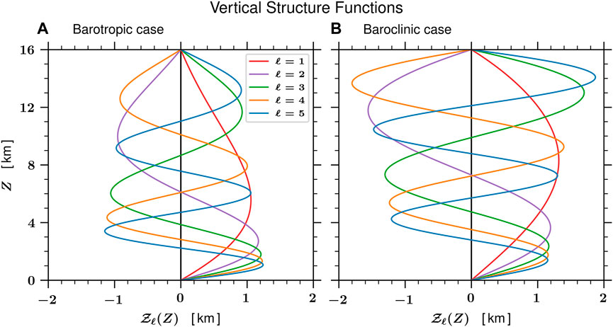
FIGURE 8. Barotropic (A) and baroclinic (B) vertical structure functions ${\mathcal{Z}}_{\ell }(Z)$ for ℓ = 1, 2, 3, 4, 5. These are the eigenfunctions of the Sturm–Liouville problem in Eq. 23, satisfying the orthonormality relation in Eq. 40. The associated eigenvalues are given in the top (barotropic) and bottom (baroclinic) halves of Table 1.

Using Eq. 28, along with the derivative relation d [RI₁(μ_ℓR)]/dR = μ_ℓRI₀(μ_ℓR), it can be shown that the formula for ρW(R, Z) is

$\begin{array}{ll}\hfill & \rho W\left(R,Z\right)=\sum _{\ell =1}^{\infty }{A}_{\ell }\frac{{\mu }_{\ell }{I}_0\left({\mu }_{\ell }R\right)}{I_1\left({\mu }_{\ell }{R}_{\text{ew}}\right)}{\mathcal{Z}}_{\ell }\left(Z\right)\hfill \\ \hfill & \text{for}0\le R\le R_{\text{ew}}\text{and}0\le Z\le Z_{\text{T}},\hfill \end{array}(30)$

and the formula for ρw(r, z) is

$\begin{array}{ll}\hfill & \rho w\left(r,z\right)=\left(\frac{\widehat{f}\left(z\right)}{f}\right)\sum _{\ell =1}^{\infty }{A}_{\ell }\frac{{\mu }_{\ell }{I}_0\left({\mu }_{\ell }{\left[\widehat{f}\left(z\right)/f\right]}^{1/2}r\right)}{I_1\left({\mu }_{\ell }{\left[\widehat{f}\left(z\right)/f\right]}^{1/2}{r}_{\text{ew}}\left(z\right)\right)}{\mathcal{Z}}_{\ell }\left(z\right)\hfill \\ \hfill & \text{for}0\le r\le r_{\text{ew}}\left(z\right)\text{and}0\le z\le z_{\text{T}}.\hfill \end{array}(31)$

Note that the vertical mass flux ρw is related to the vertical p-velocity by ρw = −(1/g)ω and that w(r, z) can have a quite different vertical dependence than W(R, Z), for example due to the leading $\widehat{f}(z)/f$ factor, which can have large values in the lower troposphere.

We now specify Ψ_ew(Z) in such a way that it vanishes at Z = 0, Z_T and has only one local minimum for 0 < Z < Z_T. The specification of Ψ_ew(Z) constrains the problem in an important way. To see this, note that

$\begin{array}{ll}\hfill 2\pi {\int }_0^{r_{\text{ew}}\left(z\right)}\rho wrdr& =2\pi {\int }_0^{R_{\text{ew}}}\rho WRdR\hfill \\ \hfill & =2\pi {\int }_0^{R_{\text{ew}}}\frac{\partial \left(R\mathrm{\Psi }\right)}{\partial R}dR=2\pi R_{\text{ew}}{\mathrm{\Psi }}_{\text{ew}}\left(Z\right),\hfill \end{array}(32)$

which shows that the specification of 2πR_ewΨ_ew(Z) is equivalent to specification of the vertical distribution of the horizontally integrated vertical mass flux in the eye. However, the details of the spatial distribution of vertical motion in the eye comes from the elliptic equation, whose solution yields Eqs. 30 and 31. In order to make the height of the minimum value of Ψ_ew(Z) adjustable, we have chosen the form

${\mathrm{\Psi }}_{\text{ew}}\left(Z\right)={\mathrm{\Psi }}_{\text{ew}}\left(Z_{\text{m}}\right)\exp \left(\frac{\pi \left(Z_{\text{m}}-Z\right)/Z_{\text{T}}}{\tan \left(\pi Z_{\text{m}}/Z_{\text{T}}\right)}\right)\frac{\sin \left(\pi Z/Z_{\text{T}}\right)}{\sin \left(\pi Z_{\text{m}}/Z_{\text{T}}\right)},(33)$

where the specified parameter Z_m is the height of the minimum value of Ψ_ew(Z). In all the results presented here, the normalization factor Ψ_ew(Z_m) has been chosen such that 2πR_ewΨ_ew(Z_m) = −1.8 × 10⁹ kg s⁻¹. Plots of Ψ_ew(Z)/Ψ_ew(Z_m) for the two choices Z_m = 0.5 Z_T = 8 km (a middle-tropospheric forcing case) and Z_m = 0.25 Z_T = 4 km (a lower-tropospheric forcing case) are shown in Figure 9. The normalization factor chosen here results in horizontally averaged eye subsidence rates, defined by $\bar{w}(z)=[2/r_{\text{ew}}^2(z)]{\int }_0^{r_{\text{ew}}(z)}w(r,z)rdr$, of approximately 1–2 m s⁻¹, which is consistent with the aircraft observations reported by Jorgensen (1984). The projection of these two Ψ_ew(Z) profiles onto the first five vertical modes, as computed from Eq. 29, is shown in Table 1.

FIGURE 9

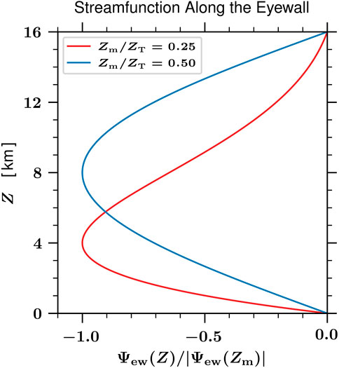
FIGURE 9. The specified function Ψ_ew(Z)/Ψ_ew(Z_m), as given by Eq. 33, for Z_m = 0.5 Z_T = 8 km and Z_m = 0.25 Z_T = 4 km. In all the results presented here we have chosen the normalization factor Ψ_ew(Z_m) such that 2πR_ewΨ_ew(Z_m) = −1.8 × 10⁹ kg s⁻¹. According to Eq. 32, the vertical distribution of the horizontally integrated downward mass flux in the eye is given by 2πR_ewΨ_ew(Z). Specification of the constant R_ew also specifies r_ew(z) since $r_{\text{ew}}(z)={[f/\widehat{f}(z)]}^{1/2}{R}_{\text{ew}}$. Determination of the detailed spatial distribution of the downward mass flux ρw(r, z) = ∂[rψ(r, z)]/r∂r requires solution of the homogeneous, restricted elliptic problem given in Eq. 16 for Ψ(R, Z), from which ψ(r, z) is obtained via ψ(r, z) = (R/r)Ψ(R, Z).

Figure 10 shows isolines of rψ(r, z) for the middle-tropospheric eyewall forcing case Z_m = 8 km (upper two panels) and for the lower-tropospheric eyewall forcing case Z_m = 4 km (lower two panels). These isolines of rψ have been computed from Eqs. 28 and 29 using the relation rψ = RΨ. The sum over ℓ in Eq. 28 has been truncated at ℓ = 20. Also shown in Figure 10 are isolines of θ(r, z); these isolines are identical to those shown in Figure 7. Alternative views of the adiabatic temperature changes in the eye are provided by (∂θ/∂t), the tendency at fixed radius r, and by (∂θ/∂τ), the tendency at fixed potential radius R. Here, we discuss only the tendency (∂θ/∂t), which is governed by

$\begin{array}{ll}\hfill \frac{\partial \theta }{\partial t}=-u\frac{\partial \theta }{\partial r}-w\frac{\partial \theta }{\partial z}& =-\frac{1}{\rho }\frac{\partial \left(r\psi ,\theta \right)}{r\partial \left(r,z\right)}\hfill \\ \hfill & =-\frac{1}{\rho }\frac{\partial \left(R\mathrm{\Psi },\theta \right)}{R\partial \left(R,Z\right)}\left(\frac{f+\zeta }{f}\right).\hfill \end{array}(34)$

FIGURE 10

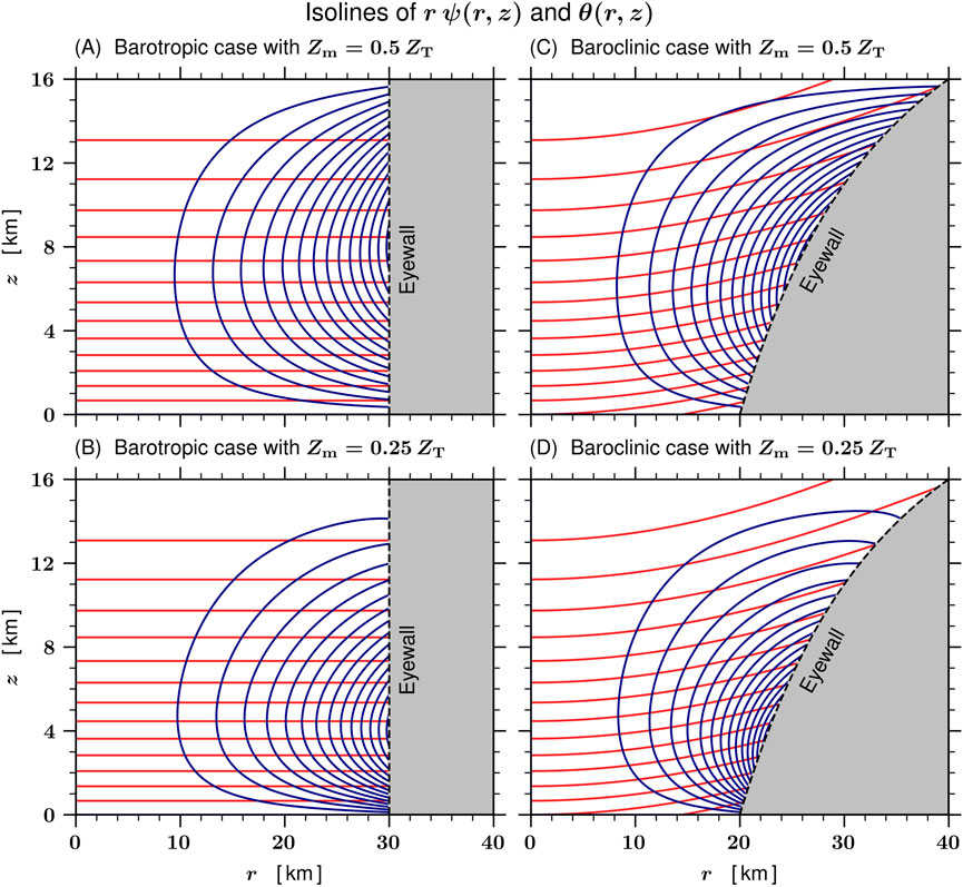
FIGURE 10. Isolines of the solution rψ(r, z) (navy blue contours) and of θ(r, z) (red contours) for the barotropic case (A,B) and for the baroclinic case (C,D), both shown for the two eyewall forcing cases Z_m = 0.5 Z_T = 8 km (A,C) and Z_m = 0.25 Z_T = 4 km (B,D). The specified functions Ψ_ew(Z) for these two eyewall forcing cases are shown in Figure 9. The isolines of rψ have been computed from the solution given in Eq. 28 using the relation rψ = RΨ, with the sum over ℓ truncated at ℓ = 20. The blue contours for rψ indicate the direction of fluid flow for the secondary circulation within the eye and have a contour interval of 2.0 × 10⁷ kg s⁻¹. The red contours for θ(r, z) are identical to those shown in Figure 7 and run from 305 K to 365 K for the barotropic case (left column) and from 295 K to 365 K for the baroclinic case (right column), both in increments of 5 K. In regions where a small area is enclosed by two neighboring blue lines and two neighboring red lines, the Jacobian ∂(rψ, θ)/r∂(r, z) tends to be large, so that ∂θ/∂t tends to be large, as shown in Figure 11.

From the above Jacobian form in (r, z), we conclude that the formation of lower-tropospheric warm-ring structures, where (∂θ/∂t) is large, tends to occur where small areas are produced by the intersection of θ-isolines and (rψ)-isolines. Figure 11 shows the corresponding potential temperature tendencies produced by the secondary circulations shown in Figure 10. The lower-tropospheric baroclinic case Z_m = 4 km, shown in Figure 11D, clearly illustrates the tendency to produce an upper-tropospheric warm-core and a lower-tropospheric warm-ring structure. For example, at z ≈ 10 km, the values of ∂θ/∂t are uniform for 0 < r < 15 km and somewhat smaller for 15 < r < 28 km. In contrast, at z ≈ 3 km, the values of ∂θ/∂t near r ≈ 21 km are approximately five times as large as those at r = 0. These results indicate that a full-tropospheric warm-core structure such as that shown in Figure 10D could transform into a lower-tropospheric warm-ring structure very quickly, perhaps in less than an hour.

FIGURE 11

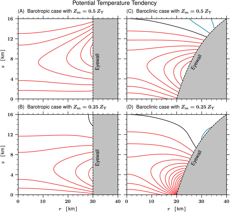
FIGURE 11. The potential temperature tendency ∂θ/∂t for the barotropic case (A,B) and for the baroclinic case (C,D), both shown for the two eyewall forcing cases Z_m = 0.5 Z_T = 8 km (A,C) and Z_m = 0.25 Z_T = 4 km (B,D). The contour interval for ∂θ/∂t is 5.0 K h⁻¹ with positive contours shown in red, the zero contour level shown in black, and negative contours shown in blue. The − w(∂θ/∂z) term contributes to positive (∂θ/∂t) at all radii and all levels, except in a small region of the upper troposphere in the baroclinic cases. In the two baroclinic cases the − u(∂θ/∂r) term generally opposes the − w(∂θ/∂z) at upper-tropospheric levels (i.e., radial advection of colder air), but enhances the − w(∂θ/∂z) term at lower-tropospheric levels (i.e., radial advection of warmer air). This results in a (∂θ/∂t) field that is more radially uniform in the upper troposphere, but enhanced near the edge of the eye at lower-tropospheric levels.

4 Concluding remarks

Two problems for the secondary circulation in R-space have been formulated. The first is the full domain elliptic problem (Eq. 15), which requires knowledge of the coefficients $\widehat{f}(R,Z)$ and N(R, Z), and the forcing Q(R, Z) over 0 ≤ R < ∞. The second is the restricted domain elliptic problem (Eq. 16), which requires knowledge of the coefficients $\widehat{f}(R,Z)$] and N(R, Z) over 0 ≤ R ≤ R_ew and specification of the lateral boundary values Ψ_ew(Z) at R = R_ew. For the barotropic vortex core and the vertically sheared Rankine core, the restricted domain elliptic problem has been solved semi-analytically in Section 3. The results for the middle-tropospheric forcing barotropic case shown in the upper left panels of Figure 10 and Figure 11 are closest to the results shown in the previous study (Schubert et al., 2007), which were based on full domain, physical space solutions of the transverse circulation equation with forcing of the first internal mode only. In the results for the lower-tropospheric forcing barotropic case shown in the lower left panels of Figure 10 and Figure 11, the minimum value of Ψ_ew(Z) has been shifted to a lower level, which has the effect of producing an enhancement of ∂θ/∂t in the lower troposphere at the edge of the eye. The results for the vertically sheared (baroclinic) Rankine core, shown in the right panels of Figure 10 and Figure 11, more realistically capture the outward tilt of the eyewall and illustrate to a greater degree the preference for the potential temperature tendency to be largest in the lower troposphere at the edge of the eye in baroclinic vortices for which the minimum value of the eyewall streamfunction Ψ_ew(Z) occurs below middle-tropospheric levels. The right two panels of Figure 11 are consistent with the concept of a potential temperature tendency field that is nearly uniform in radius at upper tropospheric levels but highly biased toward the edge of the eye at lower tropospheric levels, i.e., consistent with the development of a warm core at upper levels and a warm ring at lower levels, as seen in the full-physics simulations of Figure 5.

It is important to note that the model of eye subsidence used here is highly idealized, i.e., it is axisymmetric, gradient balanced, inviscid, adiabatic, and for a restricted domain. The adiabatic idealization results because, in the formulation of the restricted problem (Eq. 16), it has been assumed that Q = 0 for R ≤ R_ew. Careful inspection of the lower panel of Figure 4 indicates that this assumption might be violated in the upper troposphere near the edge of the eye, where frozen condensate can be advected inward and subsequently sublimated, producing a region where Q < 0. Malkus (1958), Willoughby (1998), and Zhang et al. (2002) have considered the role that such cooling might play in producing deep, narrow downdrafts at the edge of the eye. The relative roles of such diabatic dynamics and the adiabatic dynamics studied here deserve further study. The idealization of gradient balance filters inertia-gravity waves, which results in a “slow manifold” view of eye dynamics. With their mesoscale scanning techniques, the GOES-R series of geostationary satellites can image a 1000 km × 1000 km hurricane area with 30 s time resolution. When viewing such rapid-scan loops of a major hurricane, one is struck by the highly dynamic nature of the inner core. Some of the high frequency variability of the inner core is probably due to inertia-gravity wave oscillations that are not captured by the simplified dynamics of the balanced vortex model. However, the balanced vortex model does capture the slow-manifold dynamics upon which we can crudely imagine the higher frequency inertia-gravity waves are superposed. To improve this crude view, much work remains to understand how the inner core PV dynamics can become frequency matched with the inertia-gravity wave oscillations, so the two types of dynamics can evolve in a strongly coupled fashion.

In closing, we comment on the possible effects of lower-tropospheric warm-ring structure on the stadium effect. General experience with solutions of the Eliassen transverse circulation equation supports the notion that baroclinic effects play an important role in determining the outward tilt of the eyewall, as seen for example in the CloudSat observations of Figure 4. We have studied the secondary circulation in the eye when the vortex has a warm-core structure at all levels, as shown in the right panel of Figure 7. The results indicate that a lower-tropospheric warm-core structure can be modified to a lower-tropospheric warm-ring structure when the subsidence is enhanced in the lower troposphere at the edge of the eye, as shown in panels D of Figure 10 and Figure 11. When a lower-tropospheric warm ring develops in a tropical cyclone, the baroclinic terms acquire a more complicated spatial structure, which means the absolute angular momentum surfaces also acquire a correspondingly more complicated spatial structure. To see this, consider the thermal wind equation written in the form f²(R/r)³(∂R/∂z) = (g/T₀)(∂T/∂r). From this form of the thermal wind equation, we can easily deduce the following general rules.

$\begin{array}{ll}\hfill & \text{Radially\hspace{0.17em}inward\hspace{0.17em}of\hspace{0.17em}a\hspace{0.17em}warm\hspace{0.17em}ring:}\hfill \\ \hfill & \frac{\partial T}{\partial r}>0\begin{array}{cc}\hfill & \Rightarrow \frac{\partial R}{\partial z}>0\hfill \\ \hfill & \Rightarrow R-\text{surfaces\hspace{0.17em}tilt\hspace{0.17em}inward\hspace{0.17em}with\hspace{0.17em}height;}\hfill \end{array}\hfill \end{array}$

$\text{Radially\hspace{0.17em}outward\hspace{0.17em}of\hspace{0.17em}a\hspace{0.17em}warm\hspace{0.17em}ring:}$

$\begin{array}{ll}\hfill & \frac{\partial T}{\partial r}<0\begin{array}{cc}\hfill & \Rightarrow \frac{\partial R}{\partial z}<0\hfill \\ \hfill & \Rightarrow R-\text{surfaces\hspace{0.17em}tilt\hspace{0.17em}outward\hspace{0.17em}with\hspace{0.17em}height.}\hfill \end{array}\hfill \end{array}(35)$

Thus, if a tropical cyclone has a warm core at all pressure levels, the R-surfaces tilt outward with height everywhere. Since the R-surfaces help shape the secondary circulation, the eyewall updraft would generally be expected to tilt outward at all levels. However, if a tropical cyclone has a warm-core structure in the upper troposphere but a warm-ring structure in the lower troposphere, the R-surfaces tilt inward with height in the lower troposphere just inside the radius with maximum temperature anomaly. The effect is to make the secondary circulation outward-tilted at upper levels but more vertical at lower levels—an interesting refinement of the stadium effect. To better understand such refinements, additional solutions of Eq. 16 for baroclinic vortices with warm-ring structure would be helpful and are a topic for future work since such solutions would require a numerical approach to Eq. 16. The semi-analytical approach used here is restricted to the vertically sheared, Rankine vortex and simply provides a snapshot in time (rather than a complete time evolution) that illustrates the tendency for a vortex with a warm-core structure to transition to a vortex with a lower-tropospheric warm-ring structure.

Data availability statement

The original contributions presented in the study are included in this article. Further inquiries can be directed to the corresponding author.

Author contributions

WS researched and derived the scientific aspects of this work and wrote the majority of this paper. RT developed and ran the numerical models, created the figures related to those model runs, and provided editing and LaTeX support. CS assisted with the research and derivations and with the preparation of some of the figures.

Funding

Our research has been supported by the National Science Foundation under grant AGS-1841326.

Acknowledgments

We would like to thank Eric Hendricks for his helpful comments and Brian McNoldy, Natalie Tourville, and Graeme Stephens for their advice on the Typhoon Choi-Wan data. We would also like to thank Jon Martinez, Marie McGraw, and the two official reviewers for their insightful reviews and valuable suggestions. The scientific results and conclusions, as well as any views or opinions expressed herein, are those of the author(s) and do not necessarily reflect those of NOAA or the Department of Commerce.

Conflict of interest

The authors declare that the research was conducted in the absence of any commercial or financial relationships that could be construed as a potential conflict of interest.

Publisher’s note

All claims expressed in this article are solely those of the authors and do not necessarily represent those of their affiliated organizations, or those of the publisher, the editors and the reviewers. Any product that may be evaluated in this article, or claim that may be made by its manufacturer, is not guaranteed or endorsed by the publisher.

References

Aberson, S. D., Montgomery, M. T., Bell, M., and Black, M. (2006). Hurricane Isabel (2003): New insights into the physics of intense storms. Part II: Extreme localized wind. Bull. Am. Meteorol. Soc. 87, 1349–1354. doi:10.1175/BAMS-87-10-1349

CrossRef Full Text | Google Scholar

Arfken, G. B., and Weber, H. J. (2005). Mathematical methods for physicists. Sixth Edition. Amsterdam and Boston: Elsevier Academic Press.

Google Scholar

Bell, M. M., and Montgomery, M. T. (2008). Observed structure, evolution, and potential intensity of category 5 Hurricane Isabel (2003) from 12 to 14 September. Mon. Wea. Rev. 136, 2023–2046. doi:10.1175/2007MWR1858.1

CrossRef Full Text | Google Scholar

Eliassen, A. (1951). Slow thermally or frictionally controlled meridional circulation in a circular vortex. Astrophys. Norv. 5, 19–60.

Google Scholar

Fulton, S. R., and Schubert, W. H. (1985). Vertical normal mode transforms: Theory and application. Mon. Wea. Rev. 113, 647–658. doi:10.1175/1520-0493(1985)113⟨0647:VNMTTA⟩2.0.CO;2

CrossRef Full Text | Google Scholar

Hawkins, H. F., and Rubsam, D. T. (1968). Hurricane Hilda, 1964. II. Structure and budgets of the hurricane on October 1, 1964. Mon. Wea. Rev. 96, 617–636. doi:10.1175/1520-0493(1968)096<0617:hh>2.0.co;2

CrossRef Full Text | Google Scholar

Hazelton, A. T., and Hart, R. E. (2013). Hurricane eyewall slope as determined from airborne radar reflectivity data: Composites and case studies. Wea. Forecast. 28, 368–386. doi:10.1175/WAF-D-12-00037.1

CrossRef Full Text | Google Scholar

Hazelton, A. T., Rogers, R., and Hart, R. E. (2015). Shear-relative asymmetries in tropical cyclone eyewall slope. Mon. Wea. Rev. 143, 883–903. doi:10.1175/MWR-D-14-00122.1

CrossRef Full Text | Google Scholar

Johnson, R. H., and Kriete, D. C. (1982). Thermodynamic and circulation characteristics of winter monsoon tropical mesoscale convection. Mon. Wea. Rev. 110, 1898–1911. doi:10.1175/1520-0493(1982)110<1898:taccow>2.0.co;2

CrossRef Full Text | Google Scholar

Jordan, C. L. (1958). Mean soundings for the West Indies area. J. Meteor. 15, 91–97. doi:10.1175/1520-0469(1958)015<0091:MSFTWI>2.0.CO;2

CrossRef Full Text | Google Scholar

Jorgensen, D. P. (1984). Mesoscale and convective-scale characteristics of mature hurricanes. Part II: Inner core structure of Hurricane Allen (1980). J. Atmos. Sci. 41, 1287–1311. doi:10.1175/1520-0469(1984)041<1287:macsco>2.0.co;2

CrossRef Full Text | Google Scholar

Kossin, J. P., and Schubert, W. H. (2004). Mesovortices in Hurricane Isabel. Bull. Am. Meteorol. Soc. 85, 151–153.

Google Scholar

Malkus, J. S. (1958). On the structure and maintenance of the mature hurricane eye. J. Meteor. 15, 337–349. doi:10.1175/1520-0469(1958)015<0337:otsamo>2.0.co;2

CrossRef Full Text | Google Scholar

Martinez, J., Bell, M. M., Rogers, R. F., and Doyle, J. D. (2019). Axisymmetric potential vorticity evolution of Hurricane Patricia (2015). J. Atmos. Sci. 76, 2043–2063. doi:10.1175/JAS-D-18-0373.1

CrossRef Full Text | Google Scholar

Möller, J. D., and Smith, R. K. (1994). The development of potential vorticity in a hurricane-like vortex. Q. J. R. Meteorol. Soc. 120, 1255–1265. doi:10.1002/qj.49712051907

CrossRef Full Text | Google Scholar

Montgomery, M. T., Bell, M. M., Aberson, S. D., and Black, M. L. (2006). Hurricane Isabel (2003): New insights into the physics of intense storms. Part I: Mean vortex structure and maximum intensity estimates. Bull. Am. Meteorol. Soc. 87, 1335–1348. doi:10.1175/BAMS-87-10-1335

CrossRef Full Text | Google Scholar

Nolan, D. S., Stern, D. P., and Zhang, J. A. (2009a). Evaluation of planetary boundary layer parameterizations in tropical cyclones by comparison of in situ observations and high-resolution simulations of Hurricane Isabel (2003). Part II: Inner-core boundary layer and eyewall structure. Mon. Wea. Rev. 137, 3675–3698. doi:10.1175/2009MWR2786.1

CrossRef Full Text | Google Scholar

Nolan, D. S., Zhang, J. A., and Stern, D. P. (2009b). Evaluation of planetary boundary layer parameterizations in tropical cyclones by comparison of in situ observations and high-resolution simulations of Hurricane Isabel (2003). Part I: Initialization, maximum winds, and the outer-core boundary layer. Mon. Wea. Rev. 137, 3651–3674. doi:10.1175/2009MWR2785.1

CrossRef Full Text | Google Scholar

Rivoire, L., Birner, T., and Knaff, J. A. (2016). Evolution of the upper-level thermal structure in tropical cyclones. Geophys. Res. Lett. 43 (10), 537. doi:10.1002/2016GL070622

CrossRef Full Text | Google Scholar

Rogers, R. F. (2021). Recent advances in our understanding of tropical cyclone intensity change processes from airborne observations. Atmosphere 12 (650), 650. doi:10.3390/atmos12050650

CrossRef Full Text | Google Scholar

Rozoff, C. M., Schubert, W. H., McNoldy, B. D., and Kossin, J. P. (2006). Rapid filamentation zones in intense tropical cyclones. J. Atmos. Sci. 63, 325–340. doi:10.1175/JAS3595.1

CrossRef Full Text | Google Scholar

Schubert, W. H., and Alworth, B. T. (1987). Evolution of potential vorticity in tropical cyclones. Q. J. R. Meteorol. Soc. 113, 147–162. doi:10.1002/qj.49711347509

CrossRef Full Text | Google Scholar

Schubert, W. H. (2018). Bernhard Haurwitz memorial lecture (2017): Potential vorticity aspects of tropical dynamics. http://arXiv.org/abs/1801.08238.

Google Scholar

Schubert, W. H., and Hack, J. J. (1983). Transformed Eliassen balanced vortex model. J. Atmos. Sci. 40, 1571–1583. doi:10.1175/1520-0469(1983)040<1571:tebvm>2.0.co;2

CrossRef Full Text | Google Scholar

Schubert, W. H., and McNoldy, B. D. (2010). Application of the concepts of Rossby length and Rossby depth to tropical cyclone dynamics. J. Adv. Model.. Earth Syst. 2, 7. doi:10.3894/JAMES.2010.2.7

CrossRef Full Text | Google Scholar

Schubert, W. H., Rozoff, C. M., Vigh, J. L., McNoldy, B. D., and Kossin, J. P. (2007). On the distribution of subsidence in the hurricane eye. Q. J. R. Meteorol. Soc. 133, 595–605. doi:10.1002/qj.49

CrossRef Full Text | Google Scholar

Simpson, R. H., and Starrett, L. G. (1955). Further studies of hurricane structure by aircraft reconnaissance. Bull. Am. Meteorol. Soc. 36, 459–468. doi:10.1175/1520-0477-36.9.459

CrossRef Full Text | Google Scholar

Stern, D. P., Bryan, G. H., and Aberson, S. D. (2016). Extreme low-level updrafts and wind speeds measured by dropsondes in tropical cyclones. Mon. Wea. Rev. 144, 2177–2204. doi:10.1175/MWR-D-15-0313.1

CrossRef Full Text | Google Scholar

Stern, D. P., and Nolan, D. S. (2009). Reexamining the vertical structure of tangential winds in tropical cyclones: Observations and theory. J. Atmos. Sci. 66, 3579–3600. doi:10.1175/2009JAS2916.1

CrossRef Full Text | Google Scholar

Willoughby, H. E. (1998). Tropical cyclone eye thermodynamics. Mon. Wea. Rev. 126, 3053–3067. doi:10.1175/1520-0493(1998)126<3053:TCET>2.0.CO;2

CrossRef Full Text | Google Scholar

Yamasaki, M. (1983). A further study of the tropical cyclone without parameterizing the effects of cumulus convection. Pap. Meteorol. Geophys. 34, 221–260. doi:10.2467/mripapers.34.221

CrossRef Full Text | Google Scholar

Zhang, D.-L., Liu, Y., and Yau, M. K. (2002). A multiscale numerical study of Hurricane Andrew (1992). Part V: Inner-core thermodynamics. Mon. Wea. Rev. 130, 2745–2763. doi:10.1175/1520-0493(2002)130<2745:amnsoh>2.0.co;2

CrossRef Full Text | Google Scholar

Appendix A: Coordinate transformation

This appendix provides an outline of the transformation from the (r, z, t)-version of the gradient balanced model, given in Eq. 1, to the (R, Z, τ)-version, which is given in Eq. 11.

• To transform the gradient wind formula in Eq. 1, note that

$\begin{array}{ll}\hfill \left(f+\frac{v}{r}\right)v=\frac{\partial \varphi }{\partial r}& \Rightarrow \left(f+\zeta \right)v=\frac{\partial \mathrm{\Phi }}{\partial r}\hfill \\ \hfill & \Rightarrow f\frac{R}{r}v=\frac{\partial \mathrm{\Phi }}{\partial R}.\hfill \end{array}$

Using v = (R/r)V, we then obtain the first entry in Eq. 11.

• To transform the second entry in Eq. 1, we start with the absolute angular momentum form and write

$\begin{array}{ll}\hfill \frac{D\left(RV+\frac{1}{2}f{r}^2\right)}{Dt}=0& \Rightarrow \frac{DV}{Dt}+f\frac{r}{R}u=0\hfill \\ \hfill & \Rightarrow \frac{\partial V}{\partial \tau }+f\left(\frac{r}{R}u+\frac{w}{f}\frac{\partial V}{\partial Z}\right)=0\hfill \\ \hfill & \Rightarrow \frac{\partial V}{\partial \tau }+fU=0,\hfill \end{array}$

where we have made use of (Dr/Dt) = u and the absolute angular momentum conservation relation DR/Dt = 0. The final form results from the definition of U, which is given in the first entry of Eq. 10.

• To transform the hydrostatic formula in Eq. 1, note that

$\begin{array}{ll}\hfill \frac{\partial \mathrm{\Phi }}{\partial Z}& =\frac{\partial \mathrm{\Phi }}{\partial z}-\frac{\partial R}{\partial z}\frac{\partial \mathrm{\Phi }}{\partial R}\hfill \\ \hfill & =\frac{\partial \varphi }{\partial z}+v\left(\frac{\partial v}{\partial z}-f\frac{R}{r}\frac{\partial R}{\partial z}\right)=\frac{\partial \varphi }{\partial z},\hfill \end{array}$

where the second equality results from $\mathrm{\Phi }=\varphi +\frac{1}{2}{v}^2$ and the transformed gradient wind equation, while the last equality follows from cancellation of the terms within the parentheses. The third entry in Eq. 11 immediately follows. A closely related formula is

$\begin{array}{ll}\hfill \frac{\partial \mathrm{\Phi }}{\partial \tau }& =\frac{\partial \mathrm{\Phi }}{\partial t}-\frac{\partial R}{\partial t}\frac{\partial \mathrm{\Phi }}{\partial R}\hfill \\ \hfill & =\frac{\partial \varphi }{\partial t}+v\left(\frac{\partial v}{\partial t}-f\frac{R}{r}\frac{\partial R}{\partial t}\right)=\frac{\partial \varphi }{\partial t},\hfill \end{array}$

which justifies the use of the term “geopotential tendency equation” for Eq. 36.

• Interestingly, a short derivation of the fourth entry in Eq. 11 begins with the vorticity equation and proceeds as follows:

$\begin{array}{ll}\hfill & \frac{D\zeta }{Dt}+\frac{\partial w}{\partial r}\frac{\partial v}{\partial z}-\left(f+\zeta \right)\frac{\partial \left(\rho w\right)}{\rho \partial z}=0\hfill \\ \hfill & \Rightarrow \frac{D\zeta }{Dt}-\left(f+\zeta \right)\frac{\partial \left(\rho w\right)}{\rho \partial Z}=0\hfill \\ \hfill & \Rightarrow \frac{\partial }{\partial \tau }\left(\frac{f}{f+\zeta }\right)+\frac{\partial \left(\rho W\right)}{\rho \partial Z}=0,\hfill \end{array}$

where the second entry follows by combining the twisting and divergence terms and the third entry follows from the use of (D/Dt) = (∂/∂τ) + w(∂/∂Z) and the relationship between W and w. Now start with the tangential wind equation and proceed as follows:

$\begin{array}{ll}\hfill \frac{\partial V}{\partial \tau }+fU=0& \Rightarrow \frac{\partial }{\partial \tau }\left(\frac{\partial \left(RV\right)}{R\partial R}\right)+f\frac{\partial \left(RU\right)}{R\partial R}=0\hfill \\ \hfill & \Rightarrow \frac{\partial }{\partial \tau }\left(\frac{f}{f+\zeta }\right)=\frac{\partial \left(RU\right)}{R\partial R},\hfill \end{array}$

where the second entry follows by differentiation of R times the first entry, and the third entry from f²/(f + ζ) = f − [∂(RV)/R∂R]. Combining the last entries of the above two results yields the fourth entry in Eq. 11.

• Finally, the transformation of the thermodynamic equation in Eq. 1 proceeds as follows:

$\begin{array}{ll}\hfill \frac{DT}{Dt}+\frac{\kappa T}{H}w=\frac{Q}{c_{\text{p}}}& \Rightarrow \frac{\partial T}{\partial \tau }+\left(\frac{\partial T}{\partial Z}+\frac{\kappa T}{H}\right)w=\frac{Q}{c_{\text{p}}}\hfill \\ \hfill & \Rightarrow \frac{\partial T}{\partial \tau }+\frac{T}{\theta }\frac{\partial \theta }{\partial Z}w=\frac{Q}{c_{\text{p}}}\hfill \\ \hfill & \Rightarrow \frac{\partial T}{\partial \tau }+\frac{T_0}{g}{N}^{2}W=\frac{Q}{c_{\text{p}}},\hfill \end{array}$

where the final form results from the definitions of N² and W.

Appendix B: Geopotential tendency equation

The secondary circulation problems defined in Eqs. 15 and 16 were derived by eliminating Φ_τ between the two equations in Eq. 14. An alternative approach is to make use of the fourth entry in Eq. 11 to eliminate U and W between the two equations in Eq. 14, thereby obtaining the geopotential tendency equation. Then, translating the Dirichlet boundary conditions on U and W into Neumann boundary conditions on the normal derivatives of Φ_τ, the geopotential tendency problem for the restricted domain can be written as follows.

$\begin{array}{cc}\hfill & \mathbf{\text{Geopotential Tendency Problem on the Restricted Domain:}}\hfill \\ \hfill & \frac{\partial }{R\partial R}\left(\frac{R{e}^{-Z/H}}{{\widehat{f}}^2}\frac{\partial {\mathrm{\Phi }}_{\tau }}{\partial R}\right)+\frac{\partial }{\partial Z}\left(\frac{e^{-Z/H}}{N^2}\frac{\partial {\mathrm{\Phi }}_{\tau }}{\partial Z}\right)=0\hfill \\ \hfill & \text{for}0\le R<R_{\text{ew}}\text{and}0\le Z\le Z_{\text{T}}\text{with}\hfill \\ \hfill & \left\{\begin{array}{cc}\frac{\partial {\mathrm{\Phi }}_{\tau }}{\partial Z}=0\hfill & \text{at}Z=0,Z_{\text{T}},\hfill \\ \frac{\partial {\mathrm{\Phi }}_{\tau }}{\partial R}=0\hfill & \text{at}R=0,\hfill \\ \frac{\partial {\mathrm{\Phi }}_{\tau }}{\partial R}\text{\hspace{0.17em}given}\hfill & \text{at}R=R_{\text{ew}}.\hfill \end{array}\right.\hfill \end{array}(36)$

All the conclusions reached in Section 3 could also be reached through an analysis of Eq. 36.

Appendix C: Orthonormality of the vertical structure functions

The orthonormality of the vertical structure functions is proved as follows. Let ${\mathcal{Z}}_{\ell }(Z)$ and ${\mathcal{Z}}_{{\ell }^{\prime }}(Z)$ be eigenfunctions with corresponding eigenvalues μ_ℓ and μ_ℓ′. Then, multiplying the equation for ${\mathcal{Z}}_{{\ell }^{\prime }}$ by ${\mathcal{Z}}_{\ell }$, and the equation for ${\mathcal{Z}}_{\ell }$ by ${\mathcal{Z}}_{{\ell }^{\prime }}$, we obtain

$\begin{array}{ll}\hfill {\mathcal{Z}}_{\ell }\frac{d}{dZ}\left({\widehat{f}}^2{e}^{Z/H}\frac{d{\mathcal{Z}}_{{\ell }^{\prime }}}{dZ}\right)& +{\mu }_{{\ell }^{\prime }}^2{N}^2{e}^{Z/H}{\mathcal{Z}}_{\ell }{\mathcal{Z}}_{{\ell }^{\prime }}=0,\hfill \\ \hfill {\mathcal{Z}}_{{\ell }^{\prime }}\frac{d}{dZ}\left({\widehat{f}}^2{e}^{Z/H}\frac{d{\mathcal{Z}}_{\ell }}{dZ}\right)& +{\mu }_{\ell }^2{N}^2{e}^{Z/H}{\mathcal{Z}}_{\ell }{\mathcal{Z}}_{{\ell }^{\prime }}=0.\hfill \end{array}(37)$

The difference of these two equations can be written in the form

$\begin{array}{ll}\hfill & \frac{d}{dZ}\left\{{\widehat{f}}^2{e}^{Z/H}\left({\mathcal{Z}}_{\ell }\frac{d{\mathcal{Z}}_{{\ell }^{\prime }}}{dZ}-{\mathcal{Z}}_{{\ell }^{\prime }}\frac{3}{d{\mathcal{Z}}_{\ell }}dZ\right)\right\}\hfill \\ \hfill & +\left({\mu }_{{\ell }^{\prime }}^2-{\mu }_{\ell }^2\right)N^2{e}^{Z/H}{\mathcal{Z}}_{\ell }{\mathcal{Z}}_{{\ell }^{\prime }}=0.\hfill \end{array}(38)$

Integrating over Z and noting that both ${\mathcal{Z}}_{\ell }(Z)$ and ${\mathcal{Z}}_{{\ell }^{\prime }}(Z)$ vanish at Z = 0 and Z = Z_T, we obtain

$\left({\mu }_{{\ell }^{\prime }}^2-{\mu }_{\ell }^2\right){\int }_0^{Z_{\text{T}}}{\mathcal{Z}}_{\ell }\left(Z\right){\mathcal{Z}}_{{\ell }^{\prime }}\left(Z\right)N^2\left(Z\right)e^{Z/H}dZ=0.(39)$

Thus, in the absence of degenerate eigenvalues and with proper normalization of ${\mathcal{Z}}_{\ell }(Z)$, the orthonormality relation for the vertical structure functions is

${\int }_0^{Z_{\text{T}}}{\mathcal{Z}}_{\ell }\left(Z\right){\mathcal{Z}}_{{\ell }^{\prime }}\left(Z\right)N^2\left(Z\right)e^{Z/H}dZ=\left\{\begin{array}{cc}{N}_0^{2}H\hfill & \text{if\hspace{0.17em}}{\ell }^{\prime }=\ell ,\hfill \\ 0\hfill & \text{if\hspace{0.17em}}{\ell }^{\prime }\ne \ell .\hfill \end{array}\right.(40)$

The proof of the second entry in Eq. 22 is as follows. Change the dummy index ℓ to ℓ′ in the first entry of Eq. 22, multiply the resulting formula by ${\mathcal{Z}}_{\ell }(Z)N^2(Z)e^{Z/H}$, and then integrate over Z to obtain

$\begin{array}{ll}\hfill & {\int }_0^{Z_{\text{T}}}\mathrm{\Psi }\left(R,Z\right){\mathcal{Z}}_{\ell }\left(Z\right)N^2\left(Z\right)e^{Z/H}dZ\hfill \\ \hfill & =\sum _{{\ell }^{\prime }=1}^{\infty }{\mathrm{\Psi }}_{{\ell }^{\prime }}\left(R\right){\int }_0^{Z_{\text{T}}}{\mathcal{Z}}_{\ell }\left(Z\right){\mathcal{Z}}_{{\ell }^{\prime }}\left(Z\right)N^2\left(Z\right)e^{Z/H}dZ\hfill \\ \hfill & =N_0^{2}H{\mathrm{\Psi }}_{\ell }\left(R\right),\hfill \end{array}(41)$

where the final equality follows from the orthonormality relation (Eq. 40).