 Thibault Candela
 A. G. Chitu1
 Peter A. Fokker
- 1TNO, Geological Survey of the Netherlands, Utrecht, Netherlands
- 2Utrecht University, Department of Geosciences, Utrecht, Netherlands
Surface movement can be induced by many human subsurface activities: production of natural gas, geothermal heat extraction, ground water extraction, phreatic groundwater level lowering, storage of natural gas and CO2. In this manuscript, we focus on subsidence caused by gas production. While geological interpretations, seismic campaigns and flow modeling often provide a relatively rich pre-existing knowledge, understanding of the driving mechanisms for production-induced subsidence is still poor and forecasts are often very uncertain. This is related to the multiple poorly constrained models that translate gas production to ground surface displacements. Currently, a biased constraint of these models is inferred by arbitrarily pre-selecting a subset of those. Here, we have devised and deployed an integrated approach of the entire chain of models from the flow simulations to the ground surface displacements which, for the first time, accounts for all our pre-existing knowledge in terms of processes and uncertainties attached to them. More specifically for the transfer between reservoir depletion to compacting volume at depth, four reservoir-rock compaction models are a-priori considered, ranging from linear elastic model to nonlinear time-dependent viscous-type model. After assimilation of the geodetic observations (i.e., the ground-surface displacements) with ensemble-smoother algorithms, we demonstrate that even when all the a-priori known complexities were present in all steps of the modelling chain, the model parameter uncertainties of each model could be reduced. Interestingly we demonstrate that one can discriminate which reservoir-rock compaction model driving subsidence is activated at depth. This identification of the activated compaction model at depth is crucial to build confidence in our subsidence forecasts. The predictive power of the integrated approach is demonstrated with an ensemble of synthetic but complex reservoir flow simulations mimicking all the characteristics and uncertainties representative for real gas fields in the north of the Netherlands.
Introduction
Various types of energy-related anthropogenic subsurface activities, such as reservoir gas production, geothermal heat extraction, ground water extraction, storage of natural gas or CO2, can lead to surface movement (Zoback 2007). The relatively rich pre-existing knowledge of the underground around anthropogenic subsurface activities (e.g., through geological interpretations of seismic campaigns, borehole analysis, and reservoir flow modelling, e.g., see NAM 2016 for the Groningen gas field, the Netherlands) could make one think that the driving physical processes of anthropogenically-induced subsidence are well constrained. This is unfortunately not the case and the contribution of multiple driving physical processes is still highly debated (e.g., Mossop and Segall 1999; van Thienen-Visser et al., 2015a; Fokker et al., 2016).
In this contribution we focus on one instance of anthropogenic subsurface activities which can potentially lead to subsidence: reservoir gas production. During the extraction of natural gas from a gas field, the reservoir pressure decreases, leading to compaction. This reduction in volume at reservoir depth may induce surface subsidence (Doornhof 1992), with consequences for the environment and for human activities (e.g., van Thienen-Visser et al., 2015b; Simeoni et al., 2017). The consequences of reservoir production and its changes call for subsidence forecasting approaches. However, the link between reservoir production and subsidence is non-trivial. Some gas fields in the Netherlands and elsewhere in the world have shown a non-linearity between pressure depletion and subsidence, or even a delay between the start of production and the onset of subsidence and a continuation of subsidence even after production had stopped (Hettema et al., 2002; van Thienen-Visser et al., 2015a). This non-linear relationship between reservoir production and subsidence has been explained by the potential delay between reservoir depletion and compaction and multiple reservoir-compaction models have been already developed (e.g., Mossop 2012; De Waal 1986; NAM 2015; Pijnenburg et al., 2018, 2019). An efficient procedure to discriminate which compaction model is the most likely to explain the subsidence observations is a crucial step to gain confidence in our subsidence predictions. Defining and describing this procedure is the objective of the current contribution.
Subsidence caused by gas extraction is the result of multiple inter-connected physical processes: from the flow of fluids within the reservoir to the ground surface lowering and in between the reservoir rock compaction. As in many scientific realms, like weather forecasting and hydrology, each of these processes is attached to uncertainties which must be honored. In this regard a probabilistic ensemble-based approach (e.g., Reggiani and Weerts 2008; Jaynes 2003, Evensen 2003; Emerick and Reynolds 2013a; Emerick and Reynolds 2013b) can be appropriate and fruitful. An “ensemble” here implies that we build multiple subsidence realizations, based on the possible choices of processes and subsurface parameters. Later, deploying an ensemble-smoother algorithm, this prior ensemble is confronted with the subsidence observations to refine the predictions and to identify the most likely driving processes; and more specifically in our case to discriminate which compaction model is the most likely to explain the subsidence observations.
Ensemble-based inversion procedures of surface subsidence have already been developed in the past (see e.g., Fokker et al., 2012; Baù et al., 2015; Fokker et al., 2016; Gazzola et al., 2021). However, these pioneering works were designed for specific applications, where the full spectrum of uncertainties from the reservoir flow to the modelling of subsidence was not accounted for. A-priori omitting additional complexities of potentially activated processes, the “apparent” constraint of the subset of uncertain models was thus biased. For example (Fokker et al., 2016) assumed a linear compaction model and only varied the reservoir compaction coefficient and the subsurface elastic moduli. Instead in the present contribution our objective is to introduce an integrated approach, coined Ensemble-based Subsidence Interpretation and Prediction (ESIP), which honors all the pre-existing known complexities in terms of processes and subsurface parameters.
For evaluation purposes, our integrated approach is applied on numerical flow simulations aiming to mimic the characteristics of real gas fields in the north of Netherlands. First, we describe our fit-for-purpose exercise and the challenges attached to it. Second, we describe the integrated approach from each forward model to the inversion procedure. Third, the results of the integrated approach applied on our tailored exercise are presented and discussed. We demonstrate that while accounting for all the pre-existing known complexities, our integrated approach enables to identify the correct compaction process activated at depth.
Description of the Exercise and Challenges
In the exercise we designed we use the reservoir flow model of a typical gas field in the north of the Netherlands. The complexities of such a field are reproduced with a synthetic reservoir model, and multiple reservoir simulations are performed to mimic the prevalent uncertainty. One of the realizations is selected as the synthetic truth model and used for creating synthetic subsidence data, while the others are employed to show how the knowledge about the reservoir compaction and the subsidence forecasting can be improved with these data.
It is often the case that over-simplified synthetic reservoir models are used for testing purposes. This is the case of the simplified disk-shaped reservoir with spatially uniform pressure drop presented by Baù et al. (2015). Instead here our synthetic reservoir model preserves all the complexities of a real gas field (see Section 3.1) in terms of geometry and spatio-temporal pressure drop history.
Making use of model-based synthetic subsidence data presents pros and cons. The main inconvenient is that synthetic data can be missing additional complexities that are unmapped in our model-based simplified version of the reality. However, it is important to stress that for our exercise these additional complexities were accounted for by an appropriate evaluation of the uncertainties of the observations formalized with the full data covariance matrix (see Section 3.6). The main advantage of using synthetic data is that in our model-based realm, one can virtually control everything and thus it makes it ideal for testing purposes. More specifically in contrast to real data, we know upfront which processes and parameters are at the origin of the synthetic data. One can thus test if our integrated approach can effectively recover these processes and parameters.
Our exercise aims to estimate and forecast ground-surface displacements from 2008 to 2015 based on synthetic data from 1986 to 2007. We ran reservoir simulations for multiple scenarios from 1986 to 2015. Because the synthetic data correspond to one member of the prior ensemble, we have data and models from 1986 to 2015. Our predictions from 1986 to 2015, based on model conditioning from 1986 to 2007, can therefore be directly checked against our synthetic measurements from 1986 to 2015.
Besides testing the predictive and forecasting capabilities of our integrated approach, the prime scientific challenge that we are tackling with our exercise is: does our integrated approach combining forward models (and their uncertainties) with ensemble-smoother algorithms help to discriminate which type of compaction model best explains the synthetic data? Four types of compactions models, ranging from linear elastic model to nonlinear time-dependent viscous-type model, were considered: the linear, the bilinear, the time decay, and the rate type model (see Section 3.3). We selected the bilinear compaction model to generate the synthetic data and thus the goal of the exercise is to test if our integrated approach enables to retrieve this information.
Description of the Integrated Approach
This section details the integrated approach that we designed to constrain the compaction process at depth and consequently to improve forecasting capability of subsidence. The goal of our ensemble-based integrated approach is first to perform a global uncertainty analysis where all the uncertain parameters of each process of the entire chain of models are vary simultaneously. The succession of processes to be modelled is: 1) flow of fluids within the reservoir, 2) compaction at depth of the reservoir caused by pressure depletion, 3) ground surface displacement caused by the reservoir compaction and mechanical response of the surrounding medium around it. For each of these processes, multiple parameters can be involved. The a-priori range and distribution of each of these model parameters is pre-defined by our expert knowledge and the pre-existing literature for our case-study: typical gas fields in the north of the Netherlands. The distribution of each model parameter is uniform, and we use the Latin hypercube sampling method to randomly select parameter values from the overall multidimensional distribution.
Ensemble of Pressure-Depletion Scenarios
A synthetic gas field was built with Shell’s propriety reservoir simulator MoReS, mimicking the complexities of a typical real field in the north of the Netherlands. These complexities (see Figure 1) are: 1) a fault potentially compartmentalizing the reservoir with an uncertain sealing capacity (that is an uncertain fault transmissibility mapped into a fault permeability multiplier with an uniform a-priori distribution between
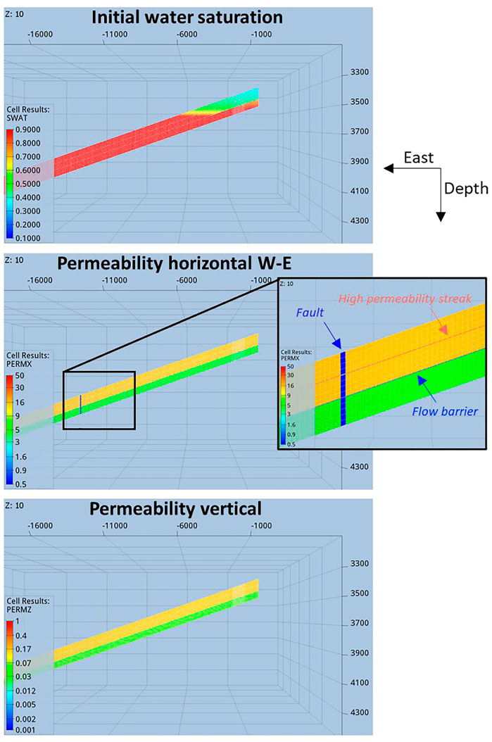
FIGURE 1. Cross-sections of the reservoir and connected aquifer for one member of the ensemble of flow simulations. Top: initial water saturation (fraction of the pore space occupied by water) of the model indicating the progressive interface between reservoir (west side) and aquifer (east side). Middle/Bottom: horizontal/vertical permeability-structures (in mD).
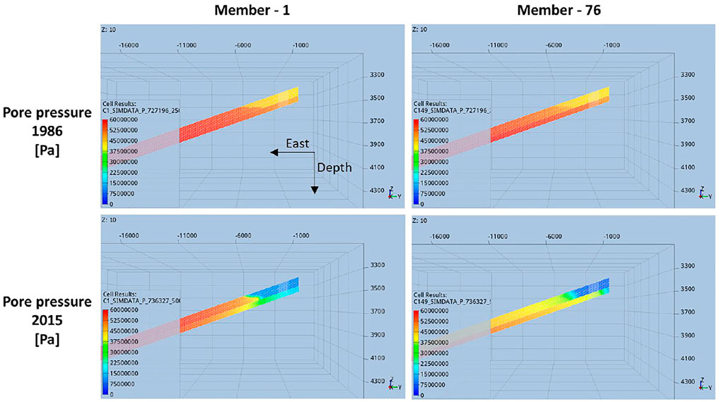
FIGURE 2. Cross-sections of the pore pressure distribution in the reservoir and connected aquifer for two members of the ensemble of flow simulations. Top: pore pressure pre-production [1986]. Bottom: pore pressure at the end of production [2015].
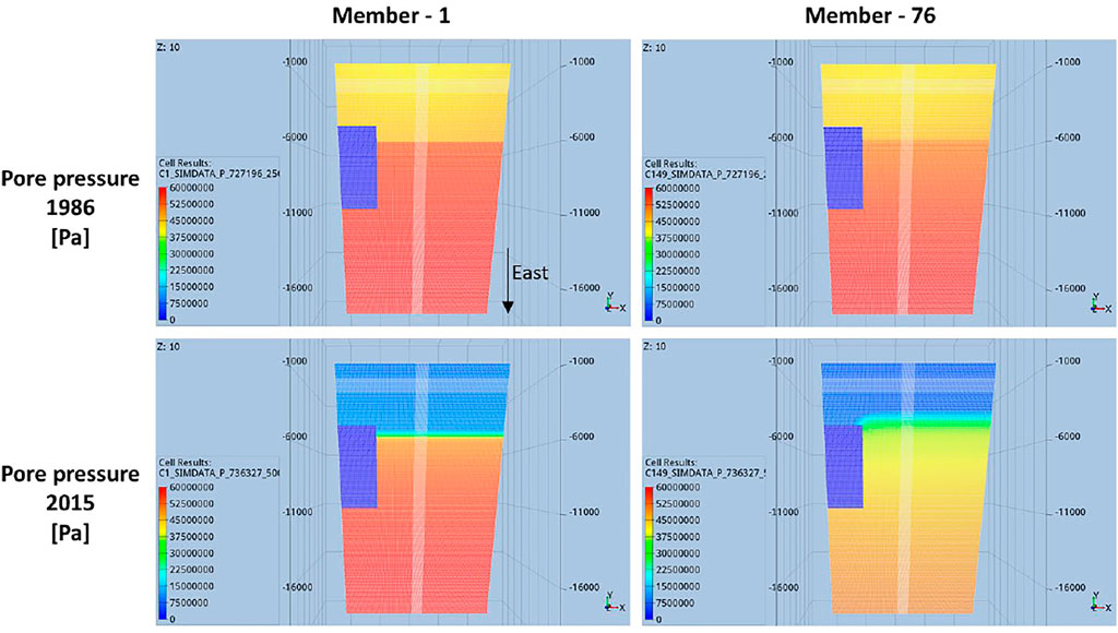
FIGURE 3. Top-views of the pore pressure distribution in the reservoir and connected aquifer for two members of the ensemble of flow simulations. Top: pore pressure pre-production [1986]. Bottom: pore pressure at the end of production [2015]. The blue rectangle of zero pore pressure, on the south-side of the model, corresponds to an intentionally cropped-volume (non-active zone) intended to mimic the complex geometry of real field cases. Still for the sake of capturing structural complexities of real field cases, east-west and north-south corridors of relatively smaller grid-block volumes are also visible.
Upscaling
The 3-D pressure fields (Figures 1–3) are upscaled to 2-D maps in two steps: the vertical averaging of the pressure in the reservoir layers and the horizontal averaging over a coarser grid. This averaging process reduces the computational runtime and is justified by the fact that a distribution of compaction over an upscaled cell in a thin and deep reservoir has a limited effect on the surface subsidence (Geertsma, 1973).
The upscaling needs to be performed such that the amount of compaction for the upscaled 2-D grid and the initial layered 3-D grid is identical. Therefore, the vertical and horizontal averaging of the 3-D pressure field need to be weighted, to take into account the variability in compaction between each individual grid block of the reservoir model. This variability in compaction is controlled by differences in pressures, volumes, and porosities between each grid block. The vertically averaged pressures
In Equation 1
The second step of the upscaling consists in the horizontal averaging of pressures, volumes, and porosities of the 2-D fine grid
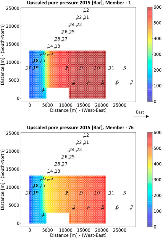
FIGURE 4. Upscaled pore pressure distributions for two members of the ensemble of flow simulations. The dark rectangles indicate the surface locations of the geodetic benchmarks; their uneven spatial distribution is mimicking real scenarios of the north of the Netherlands.
From Pressure Depletion to Compaction
Translating the pressure depletion between two epochs to volume compaction is non-trivial. Models for rock compaction based on laboratory measurements and/or field measurements are still highly debated (De Waal, 1986; Hettema et al., 2002; van Thienen-Visser et al., 2015a; NAM, 2015; Pruiksma et al., 2015; Spiers et al., 2017; van Eijs and van der Wal, 2017; Pijnenburg et al., 2018, 2019; Smith et al., 2019). For our exercise, four types of compaction models, ranging from linear elastic model to nonlinear time-dependent viscous-type model, were considered: the linear, the bilinear, the time decay, and the rate type model.
The linear elastic compaction model assumes a linear relationship between pressure depletion
where
The three other compaction models (bilinear, time-decay, rate type) intend to capture non-linear time-dependent viscous-type and/or pressure-dependent behavior. They have been formulated in response to geomechanical and geodetic measurements pointing out nonlinearities and delays in compaction and subsidence relative to the production of gas fields (De Waal, 1986; Hettema et al., 2002; van Thienen-Visser et al., 2015a; NAM, 2015; Pruiksma et al., 2015; Spiers et al., 2017; van Eijs and van der Wal, 2017). Recent observations also indicate continuing subsidence even when production has stopped.
In the bilinear compaction model (NAM 2017), the compaction coefficient is assumed to be pressure-dependent. It combines two linear relationships between pressure depletion and reservoir rock compaction as:
where
The time-decay model was inspired by the ubiquitous diffusive behavior of many physical systems pushed into non-equilibrium high-energy states, which slowly decay to their low-energy equilibrium states again (Mossop 2012). Such a diffusion-type process can be modeled using a convolution of a linear relationship between pressure depletion and reservoir rock compaction with an exponential time decay function:
where
The rate type compaction model was derived from laboratory measurements designed for capturing the loading-rate dependency in sandstones (De Waal 1986). The onset and arrest of production can be seen as changes in loading rate of the reservoir rocks. At the change in loading rate, a first direct elastic strain response
1) From the current effective vertical stress
The vertical stress is derived from the reservoir depth and the mean density
At the onset of pressure depletion/production
The reference total strain is expressed as:
with the reference vertical effective stress
Three material parameters (
2) The second step of the Euler scheme consists in calculating the increase in creep strain as:
and update the creep strain as:
3) The time is updated as
4) Following a linear stress-strain relationship one can calculate the direct elastic strain as:
5) Finally One can Calculate the Total Cumulative Strain as
And the total cumulative compaction as:
with
From Compaction to Ground-Surface Displacements
In order to propagate the 2-D compaction fields to surface subsidence we employ influence functions, also called Green functions. They are rotationally symmetric surface displacement profiles for a unit volume of compaction (a nucleus of volumetric strain) and they are used in conjunction with the 2-D compaction fields, in order to calculate the total surface displacements at the desired geodetic benchmarks locations. We used the semi-analytical approach developed by (Fokker & Orlic 2006), which is based on the nucleus of strain concept (Mindlin & Cheng 1950) and which extends Geertsma’s analytical solutions (Geertsma 1973; Van Opstal 1974) in the sense that it can handle a layered elastic subsurface. The influence functions give the vertical and horizontal surface displacements for a single “nucleus” (a unit center of compression) located at reservoir depth, and for given elastic parameters. The required input parameters are the reservoir depth, the depths of the layer interfaces, Young’s modulus and Poisson’s ratio of each layer. For the present study, an elastic two-layer subsurface model has been considered. The interface between the layers was put at −3800 m depth, 80 m below the reservoir (−3720 m). Uncertainties of the model parameters (Young’s modulus and Poisson’s) of both layers have been mapped out in the prior ensembles (see Section 3.5) to cover the broad range of possibilities from a homogeneous elastic subsurface (no elastic differences between both layers) to a subsurface with a stiff basement (that is with a strong contrast of elasticity between the top and bottom layer).
Prior Predictions
For each type of compaction model and based on the prior information, a prior model vector ensemble of
The prior distributions of all the model parameters used for the compaction models and influence function are presented respectively in Tables 1, 2. For some model parameters, stochastic factors are employed to generate the prior ensembles. The prior ensembles of some compaction coefficients (

TABLE 1. Bounded uniform prior distributions for each model parameters used to build each type of compaction models.
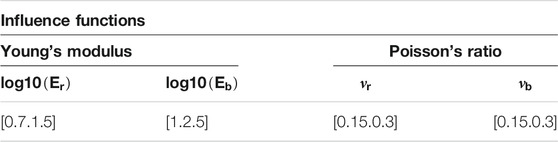
TABLE 2. Bounded uniform prior distributions for each model parameters used to build the semi-analytical influence functions for an elastic two-layers cake subsurface model. The subscript “r” indicates the elastic properties of the top layer (from the ground surface to depth −3800 m). The subscript “b” indicates the elastic properties of the bottom layer (from −3800 m to an infinite depth).
From our a-priori knowledge one can generate an ensemble of surface displacements predictions for each component of surface displacements (horizontal displacement in West-East direction u1 an North-South direction u2, and vertical displacement u3) at the specific measurement locations, that is the geodetic benchmarks locations. From these ensembles of surface displacements one can generate a prior ensemble of 90 double differences for the training period [1986–2007]. A double difference indicates a difference in time of a level difference in space (van Leijen et al., 2017), which circumvents the effect of the choice of references in time and space. In other words, one double difference is the difference of ground surface displacements (either vertical or horizontal displacements) between two benchmarks locations and between two epochs/times of geodetic campaigns. The combinations of modeled 90 double differences (in terms of benchmark locations and time of the geodetic campaigns) correspond to those of the measured (synthetic in our case) 90 double differences (see Section 3.6). These 90 double differences include all the benchmark locations presented in Figure 4.
The geomechanical forward model (compaction model + influence function) is indicated by the function
For each type of compaction model one can define a mean and a covariance matrix of the prior double differences predictions. The mean over the
The covariance over the
which can be written in matrix notation as:
And where
The mean of the priors
Geodetic Observations
Two types of ground-surface displacement measurements are considered for our exercise: optical levelling and GPS. Their spatial distribution with regard to the reservoir mimics real cases of the north of the Netherlands (Figure 4). The levelling measurements give vertical displacements only (subsidence or heave, indicated by u3); GPS also measures the horizontal displacements (West-East component u1, and North-South u2). The additional assimilation of the horizontal displacements is particularly interesting for constraining the shape of the subsidence bowl. Our integrated approach allows flexible incorporation of other measurement types like InSAR, if necessary.
The selected 90 double differences for the training period [1986–2007], and including both optical levelling and GPS, were chosen from one member (which was not used anymore in the further analysis) of the prior ensemble of the bilinear compaction model.
Along with the simulated observations, the uncertainties of the observations due to measurement noise, and temporal and spatio-temporal idealization noise were considered, formalized with the full data covariance matrix according to (van Leijen et al., 2017). A detailed description of the method used to simulate the noise of the measurements and the full covariance matrix is beyond the scope of the present publication. We simply note here that the full data-covariance matrix, describing the uncertainty/variance of each measurement, but also the temporal and spatio-temporal correlations between the measurements, even if often neglected (e.g., Fokker et al., 2012), is essential for a proper conditioning of the model parameters. Indeed, the data covariance matrix is key to properly weight the relative importance of each measuring point during the conditioning step (see later Section 3.7).
Figure 5 presents the full data covariance matrix of the 90 double differences for the training period [1986–2007]. The temporally correlated idealization noise, mostly giving positive off-diagonal numbers, describes the effect of benchmark instability. Most negative off-diagonal numbers are related to the spatio-temporal components reflecting additional surface motion not associated with the signal of interest, e.g., compaction of shallow soft soil layers. Additional complexities, such as additional ongoing processes which are not mapped in our forward modelling strategy, are thus accounted for in our integrated approach by the data covariance matrix.
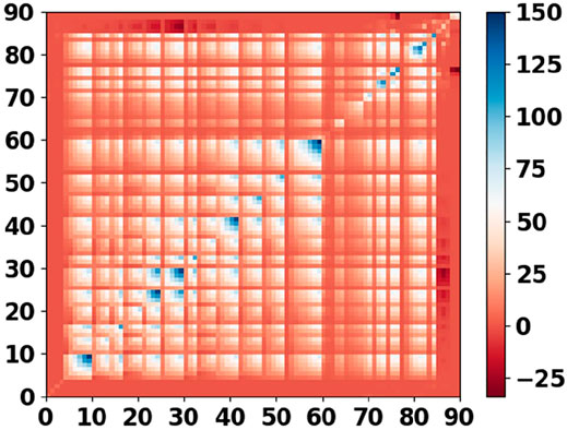
FIGURE 5. Full covariance matrix of the 90 double differences (in mm2).
Conditioning of the Models With the Data
The next step consists in confronting or conditioning the prior estimates up to T1 with the geodetic data acquired up to T1 (that is from 1986 to 2007 [1986–2007]).
The ensemble-smoother algorithm consists in an inversion scheme, for which the goal is to maximize an objective function J (or minimize–log [J]) of the form (Menke 1989; Tarantola 2005):
where
In other words, the objective function is integrated in an inversion scheme seeking the solution for the vector
The optimal “least-square” solution of Equation 24 for one particular realization and assuming a linear inverse problem is given by Tarantola (2005):
Converting this expression into an ensemble expression, we can translate this equation to a forward model that does not have to be a matrix multiplication–i.e., using the equation
which can be rewritten as:
In Equation 27
After the data assimilation step has been performed, that is computing Equation 27, posterior model parameters included in
The non-linearity in the geomechanical forward model can be more appropriately handled by applying multiple steps of data assimilation, so called Ensemble Smoother with Multiple Data Assimilation (ES-MDA) (Emerick and Reynolds 2013a). In ES-MDA, the output ensemble of the smoother is used as input for the next update. The same data are used for all assimilation steps; to compensate for the effect of the multiple application, the data covariances used in the update steps are increased with respect to its actual value. For each step, a data covariance multiplication factor
ES-MDA updates model parameters in a more “progressive” way, relative to the rather “aggressive” single step of the ES-SS. Indeed, even if at the end of the four steps of the ES-MDA the actual data covariance is honored, during each step of the ES-MDA the update can be seen as relatively “gentle” because of the data covariance inflation. Therefore, one can expect a higher ability of the ES-MDA for avoiding ensemble collapse. The downside of ES-MDA is that it is computationally slower; in our case, 4 times slower as we pick four steps of assimilation.
Performance Assessment
The performance of the ensemble-smoother algorithms (ES-SS and ES-MDA), in updating the prior ensembles towards posterior ensembles consistent with the data, can quantitatively be evaluated by different metrics. First we define a metric based on the Absolute Error (
A second metric, the Average Ensemble Spread (
Both metrics can be defined independently for the data
To evaluate the update of the ensemble-smoother algorithms (ES-SS and ES-MDA) we evaluate the variation between the prior and the posterior metrics with respect to the prior metrics:
A third class of quality metrics is formed by a chi-square
The chi-square test (Equations 32 and 33) judge if the model posterior predictions and the data are consistent. Loosely speaking, the average squared mismatch should be of the order of the covariance. A chi-square test close to unity means that the model ensemble is matching the data and that the quality of the match is in agreement with the error covariance of the data.
Results
This Section 4 presents all the results obtained with four prior ensembles, corresponding to each type of compaction model, and one identical member of the bilinear ensemble as data. Supplementary Appendix A.1 presents the results obtained with another set of four different prior ensembles and bilinear data. Similar conclusions can be drawn for the results presented in Section 4 and Supplementary Appendix A.1.
Model Parameters
Figures 6, 7 display the prior and posterior ensembles of model parameters for both the ES-SS and ES-MDA. The posterior ensembles are the ones inferred after calibration during the training period [1986–2007]. The less aggressive multi-step update of the ES-MDA helps to “better constrain” most of the model parameters. “Better constrain” means that the reduction of the parameters uncertainties is more effective with the ES-MDA than with the ES-SS. For the model parameters of the influence function, used to propagate the reservoir compaction in terms of ground-surface displacement, only the ratio between the Young’s modulus of the top layer (
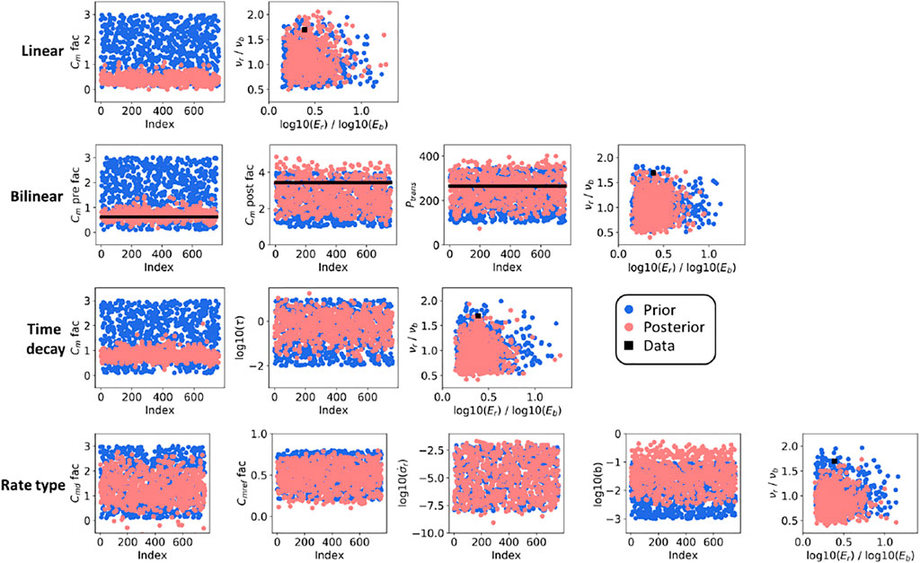
FIGURE 6. Prior and posterior (following the ES-SS algorithm and for the training period [1986–2007]) ensembles of model parameters.
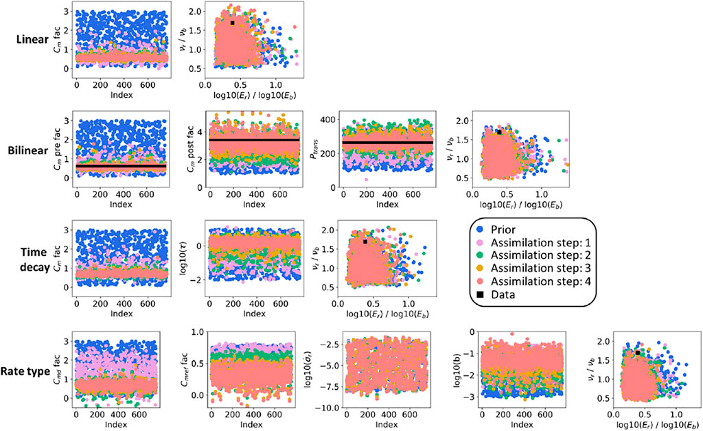
FIGURE 7. Prior and posterior (following the ES-MDA algorithm and for the training period [1986–2007]) ensembles of model parameters.
For the bilinear compaction model, where we know the true model parameters used to generate the synthetic data, the visual-inspection-based conclusion about the parameter distributions is confirmed by the metrics
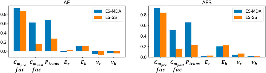
FIGURE 8.
Ground-Surface Displacements
Figures 9–12 display the prior and posterior ensembles of ground-surface displacements for both the ES-SS and ES-MDA. The results are shown for two specific geodetic benchmark locations, one on top of the reservoir (location 18, Figure 4) and one on top of the aquifer (location 8, Figure 4). The results for other geodetic benchmark locations are presented at Supplementary Appendix A.1. For both ensemble-smoother algorithms (ES-SS and ES-MDA), a qualitative assessment of the curves indicates that the spread of each posterior is smaller than the spread of their prior. The vertical ground-surface displacements of the posterior ensembles are mostly “well aligned” with the data in the sense that the spread of the posterior ensembles encompasses the data. Only for the linear compaction model, and for the combination rate-type compaction model with ES-SS, the alignment is suboptimal. With the exception of the rate-type compaction model with the ES-SS, the horizontal ground-surface displacements (West-East component u1), even if of low magnitudes, are relatively “well constrained” by the posterior ensembles for both the reservoir benchmark and aquifer benchmark.
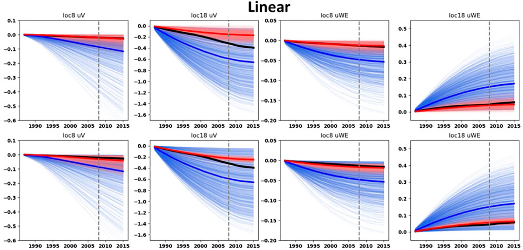
FIGURE 9. Prior and posterior ground-surface displacements for the linear ensembles. Thin blue curves: prior ensembles. Thin red curves: posterior ensembles. Blue thick curves: mean of the prior ensembles. Red thick curves: mean of the posterior ensembles. Dark thick curves: data. Top row: with the ES-SS algorithm. Bottom row: with the ES-MDA algorithm and with the posterior obtained after four steps of data assimilation. On top of each graph the benchmark location (see Figure 4) and the component of the ground-surface displacement is indicated. The vertical dashed gray line corresponds to the end of the training period.
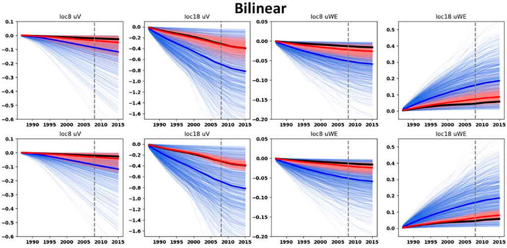
FIGURE 10. Prior and posterior ground-surface displacements for the bilinear ensembles. Thin blue curves: prior ensembles. Thin red curves: posterior ensembles. Blue thick curves: mean of the prior ensembles. Red thick curves: mean of the posterior ensembles. Dark thick curves: data. Top row: with the ES-SS algorithm. Bottom row: with the ES-MDA algorithm and with the posterior obtained after four steps of data assimilation. On top of each graph the benchmark location (see Figure 4) and the component of the ground-surface displacement is indicated. The vertical dashed gray line corresponds to the end of the training period.
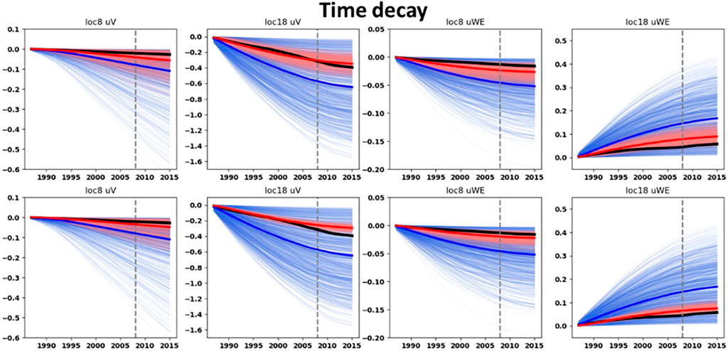
FIGURE 11. Prior and posterior ground-surface displacements for the time decay ensembles. Thin blue curves: prior ensembles. Thin red curves: posterior ensembles. Blue thick curves: mean of the prior ensembles. Red thick curves: mean of the posterior ensembles. Dark thick curves: data. Top row: with the ES-SS algorithm. Bottom row: with the ES-MDA algorithm and with the posterior obtained after four steps of data assimilation. On top of each graph the benchmark location (see Figure 4) and the component of the ground-surface displacement is indicated. The vertical dashed gray line corresponds to the end of the training period.
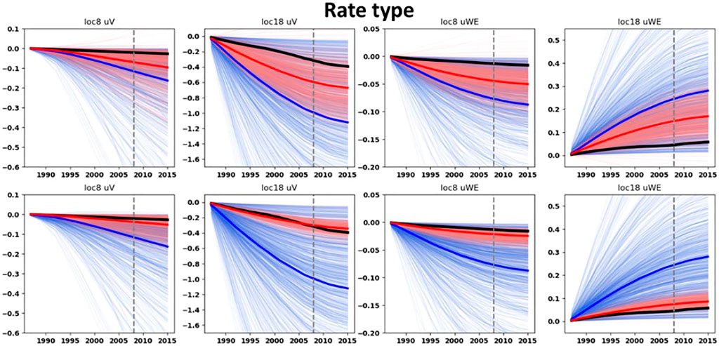
FIGURE 12. Prior and posterior ground-surface displacements for the rate type ensembles. Thin blue curves: prior ensembles. Thin red curves: posterior ensembles. Blue thick curves: mean of the prior ensembles. Red thick curves: mean of the posterior ensembles. Dark thick curves: data. Top row: with the ES-SS algorithm. Bottom row: with the ES-MDA algorithm and with the posterior obtained after four steps of data assimilation. On top of each graph the benchmark location (see Figure 4) and the component of the ground-surface displacement is indicated. The vertical dashed gray line corresponds to the end of the training period.
The posterior ground-surface displacements at the benchmark location on top of the aquifer (benchmark location 8, Figure 4) are in better agreement with the data than the movements calculated with the prior ensemble. Actually, the mean posteriors moved very close to the data during the assimilation procedure. This is remarkable given 1) the high uncertainty of the aquifer depletion and 2) the low magnitudes of the ground-surface displacements on top of the aquifer compared to those on top of the reservoir. Interestingly, for the benchmark location on top of the aquifer, the relative bandwidths of the posterior (with the ES-MDA after four steps of assimilation) horizontal ground-surface displacements (defined as the ratio between the standard deviation and the mean of the ensemble) are smaller than those of the posterior vertical displacements. As an example, for the bilinear compaction model, the relative bandwidth of the posterior horizontal ground-surface displacements on top of the aquifer is 0.57 whereas for the posterior vertical ground-surface displacements it is 1.01. This points out the importance of the use of the horizontal ground displacements to constrain the shape of the subsidence bowl on the sides of the reservoir and ultimately to constrain the aquifer activity.
For each compaction model, both metrics
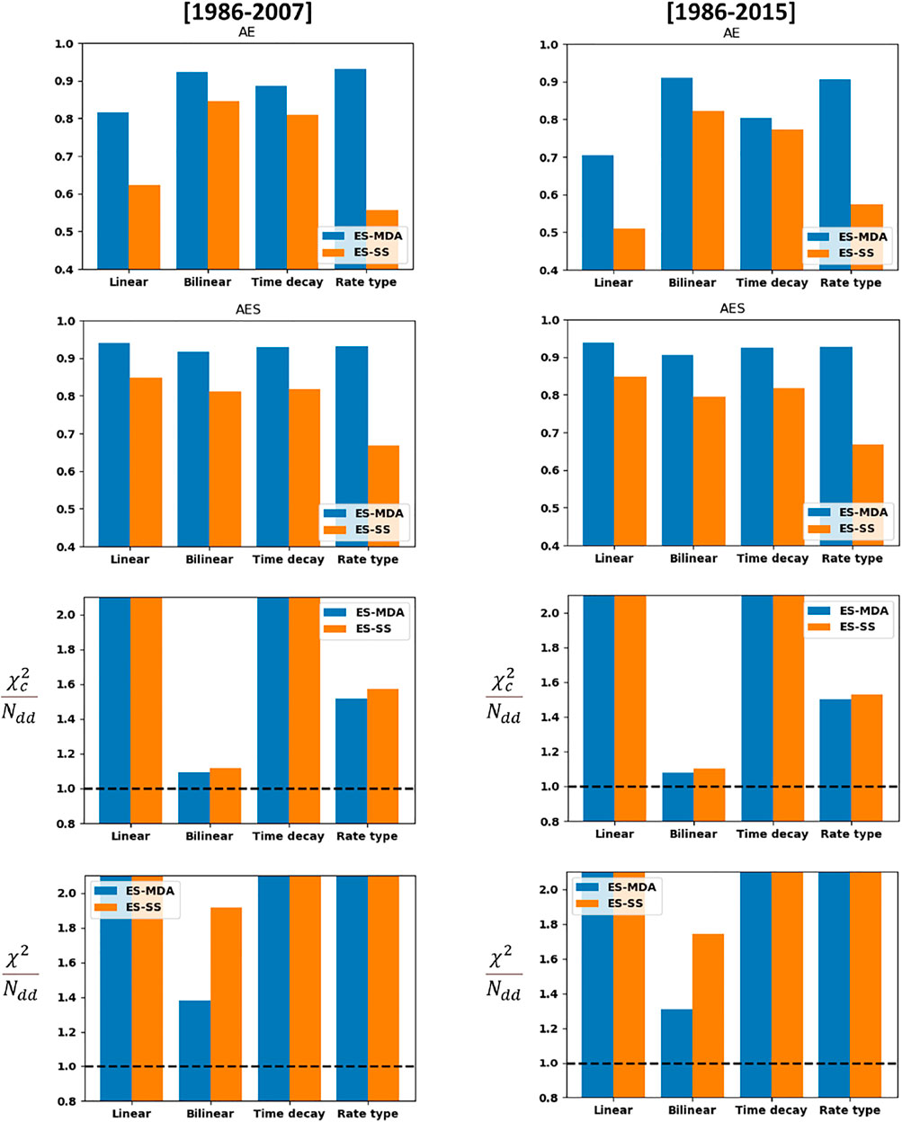
FIGURE 13.
The suboptimal update obtained with the ES-SS for the ground-surface displacements of the rate-type compaction model (Figure 12) is confirmed by the lower
An important question concerns the reliability of our subsidence forecasts. Figure 13 presents the quality metrics both for the training period [1986–2007] and for the full period [1986–2015] including the forecasting period [2008–2015], for which no measurements were used in the assimilation. We see that the metric for the full period is not significantly different from the metric for the training period. Especially the
Discussion
The main objective of our exercise was to test if our integrated approach could effectively identify the bilinear compaction model as the best compaction model to explain the synthetic data (themselves generated with a bilinear compaction model). Our analysis has demonstrated that with the combination of the
It is important to stress here that the pressure-depletion realizations were not subjected to the assimilation procedure. Even if the uncertainties in the pressure depletion were kept constant throughout the assimilation procedure, the model parameters of the bilinear compaction model were well constrained and aligned with the true-synthetic data. Both footprints in the subsidence signal, of 1) the pressure depletion and 2) the bilinear compaction, were thus effectively disentangled by our integrated approach.
In addition, our analysis has demonstrated that the update of the model parameters of the influence function is independent of the type of compaction model. Indeed, for each type of compaction model, the posterior ensembles of the Young’s modulus ratio (between the two subsurface layers) similarly converged towards the data. This last result indicates that again our integrated approach was capable to disentangle the unique footprint of the elastic layering on the subsidence signal from the footprints of the pressure depletion and compaction.
The main limitation of the current workflow is that the ensemble of reservoir flow simulations is unchanged upon assimilation. Ideally one should update the controlling reservoir parameters and make a new reservoir simulation for every ensemble member. Introducing potential future implementations, it is important to utilize the versatility of applications offered by ensemble-smoother algorithms. Our integrated approach was developed for the production of a natural gas field, but it can easily be adapted for other settings of exploitation of subsurface resources causing ground-surface movement. Typical examples are the injection of CO2 (Vasco et al., 2010), underground gas storage (Teatini et al., 2011; Castelleto et al., 2013), steam injection (Khakim et al., 2012), geothermal systems (Mossop & Segall 1999; Allis et al., 2009; Vasco et al., 2013), groundwater extraction (Galloway and Burbey 2011; Zhu et al., 2015), phreatic groundwater level management (Fokker et al., 2019) and salt mining (Fokker and Visser 2014). We have recently deployed the ES-SS to identify the driving mechanisms of induced seismicity at the Groningen gas field on a real dataset (Candela et al., 2021). This specific scenario demonstrates that the ensemble-smoother algorithms can be also applied to a discrete dataset, such as an earthquake catalog. The flexibility of the implementation of the ensemble-smoother also offers the possibility to assimilate multiple types of data. As an example, jointly assimilating subsidence geodetic observations and seismicity data, our understanding of the driving mechanisms of both induced subsidence and seismicity might be improved. An active research area in the Netherlands is the disentangling of the relative contribution between deeply seated sources of subsidence (as natural gas extraction) and shallow seated sources of subsidence (Fokker et al., 2019). These sources often interfere. Incorporating in ESIP the additional forward models for shallow seated sources of subsidence, such as soil compaction and oxidation caused by lowering of the phreatic level, might help to achieve this disentangling (Candela et al., 2020).
Conclusion
We have presented an integrated approach for subsidence evaluation, coined ESIP (Ensemble-Based Subsidence Interpretation and Prediction). The key elements of ESIP are:
- it combines fast physics-based forward models with ensemble-smoother algorithms for the data assimilation;
- it covers all the known a-priori complexities in terms of processes and subsurface parameters, and their uncertainties;
- the error covariance matrix of the subsidence data enables to properly weight the contribution of each measuring point during the conditioning;
The predictive power of ESIP has been demonstrated for a synthetic gas reservoir-aquifer system incorporating all the characteristics of real cases in the north of Netherlands. The key conclusions of the presented exercise are:
- the model parameter uncertainties of each fast forward model are reduced with the assimilation of subsidence data;
- our hindcast and forecast are improved with the assimilation of subsidence data;
- the bilinear compaction process gives the best hindcast and forecast with well-defined error bounds in agreement with the data;
- the bilinear compaction process is thus successfully identified as the driving compaction process at depth.
The identification of the driving compaction process is especially important for the subsidence forecasts. In the case of a reservoir production shutdown, the subsidence forecast obtained with each reservoir compaction model would be drastically different. As an example, for an identical pressure diffusion scenario after shutdown, the bilinear compaction model would result in a more severe subsidence than for the linear compaction model.
Data Availability Statement
The raw data supporting the conclusions of this article will be made available by the authors, without undue reservation.
Author Contributions
TC: Conceptualization, Methodology, Software, Writing-Original draft preparation. AC: Software. EP: Visualization, Writing-Original draft preparation. MP: Writing-Original draft preparation. DH: Writing-Original draft preparation. KK: Writing-Original draft preparation. PF: Supervision, Conceptualization, Methodology, Writing-Original draft preparation.
Conflict of Interest
The authors declare that the research was conducted in the absence of any commercial or financial relationships that could be construed as a potential conflict of interest.
Publisher’s Note
All claims expressed in this article are solely those of the authors and do not necessarily represent those of their affiliated organizations, or those of the publisher, the editors and the reviewers. Any product that may be evaluated in this article, or claim that may be made by its manufacturer, is not guaranteed or endorsed by the publisher.
Acknowledgments
The data generated by the integrated approach are available on request from the corresponding author.
Supplementary Material
The Supplementary Material for this article can be found online at: https://www.frontiersin.org/articles/10.3389/feart.2022.713273/full#supplementary-material
References
Allis, R., Bromley, C., and Currie, S. (2009). Update on Subsidence at the Wairakei-Tauhara Geothermal System, New Zealand. Geothermics 38, 169–180. doi:10.1016/j.geothermics.2008.12.006
Baù, D., Ferronato, M., Gambolati, G., Teatini, P., and Alzraiee, A. (2015). Ensemble Smoothing of Land Subsidence Measurements for Reservoir Geomechanical Characterization. Int. J. Numer. Anal. Meth. Geomech. 39 (2), 207–228. doi:10.1002/nag.2309
Burgers, G., Jan van Leeuwen, P., and Evensen, G. (1998). Analysis Scheme in the Ensemble Kalman Filter. Mon. Wea. Rev. 126 (6), 1719–1724. doi:10.1175/1520-0493(1998)126<1719:asitek>2.0.co;2
Candela, T., Koster, K., Stafleu, J., Visser, W., and Fokker, P. (2020). Towards Regionally Forecasting Shallow Subsidence in the Netherlands. Proc. Iahs, 382, 427–431,. doi:10.5194/piahs-382-427-2020
Candela, T., Pluymaekers, M., Ampuero, J. P., van Wees, J. D., Buijze, L., Wassing, B., et al. (2021). Controls on the Spatio-Temporal Patterns of Induced Seismicity in Groningen Constrained by Physics-Based Modeling with Ensemble-Smoother Data Assimilation. Rev. Geophys. J. Int.
Castelletto, N., Ferronato, M., Gambolati, G., Janna, C., Marzorati, D., and Teatini, P. (2013). Can Natural Fluid Pore Pressure Be Safely Exceeded in Storing Gas Underground? Eng. Geology. 153, 35–44. doi:10.1016/j.enggeo.2012.11.008
De Waal, J. A. (1986). On the Rate Type Compaction Behaviour of sandstone Reservoir rock.Doornhof, D. (1992). Surface Subsidence in the Netherlands-the Groningen Gas-Field. Geologie en Mijnbouw 71 (2), 119–130.
Doornhof, D. (1992). Surface Subsidence in The Netherlands: The Groningen Gas Field. Geologie en Mijnbouw 71, 119–130.
Emerick, A. A., and Reynolds, A. C. (2013a). Ensemble Smoother with Multiple Data Assimilation. Comput. Geosciences 55, 3–15. doi:10.1016/j.cageo.2012.03.011
Emerick, A. A., and Reynolds, A. C. (2013b). Investigation of the Sampling Performance of Ensemble-Based Methods with a Simple Reservoir Model. Comput. Geosci. 17 (2), 325–350. doi:10.1007/s10596-012-9333-z
Evensen, G. (2003). The Ensemble Kalman Filter: Theoretical Formulation and Practical Implementation. Ocean Dyn. 53 (4), 343–367. doi:10.1007/s10236-003-0036-9
Fokker, P. A., Gunnink, J. L., Koster, K., and de Lange, G. (2019). Disentangling and Parameterizing Shallow Sources of Subsidence: Application to a Reclaimed Coastal Area, Flevoland, the Netherlands. J. Geophys. Res. Earth Surf. 124. doi:10.1029/2018JF004975
Fokker, P. A., and Orlic, B. (2006). Semi-analytic Modelling of Subsidence. Math. Geol. 38 (5), 565–589. doi:10.1007/s11004-006-9034-z
Fokker, P. A., and Visser, J. (2014). Estimating the Distribution of Salt Cavern Squeeze Using Subsidence Measurements. In 48th US Rock Mechanics/Geomechanics Symposium. American Rock Mechanics Association.
Fokker, P. A., Visser, K., Peters, E., Kunakbayeva, G., and Muntendam-Bos, A. G. (2012). Inversion of Surface Subsidence Data to Quantify Reservoir Compartmentalization: A Field Study. J. Pet. Sci. Eng. 96-97, 10–21. doi:10.1016/j.petrol.2012.06.032
Fokker, P. A., Wassing, B. B. T., van Leijen, F. J., Nieuwland, D. A., and Nieuwland, D. A. (2016). Application of an Ensemble Smoother with Multiple Data Assimilation to the Bergermeer Gas Field, Using PS-InSAR. Geomechanics Energ. Environ. 5, 16–28. doi:10.1016/j.gete.2015.11.003
Galloway, D. L., and Burbey, T. J. (2011). Review: Regional Land Subsidence Accompanying Groundwater Extraction. Hydrogeol J. 19, 1459–1486. doi:10.1007/s10040-011-0775-5
Gazzola, L., Ferronato, M., Frigo, M., Teatini, P., and Zoccarato, C. (2021). “Ensemble Smoother with Multiple Data Assimilation Analysis,” in Challenges and Innovations in Geomechanics. IACMAG 2021. Lecture Notes in Civil Engineering. Editors (Springer, Cham), 125. doi:10.1007/978-3-030-64514-4_93
Geertsma, J. (1973). Land Subsidence above Compacting Oil and Gas Reservoirs. J. Pet. Tech. 25 (06), 734–744. doi:10.2118/3730-pa
Hettema, M., Papamichos, E., and Schutjens, P. (2002). Subsidence Delay: Field Observations and Analysis. Oil Gas Sci. Tech. - Rev. IFP 57 (5), 443–458. doi:10.2516/ogst:2002029
Khakim, M. Y. N., Tsuji, T., and Matsuoka, T. (2012). Geomechanical Modeling for InSAR-Derived Surface Deformation at Steam-Injection Oil Sand fields. J. Pet. Sci. Eng. 96-97, 152–161. doi:10.1016/j.petrol.2012.08.003
Mindlin, R. D., and Cheng, D. H. (1950). Nuclei of Strain in the Semi‐Infinite Solid. J. Appl. Phys. 21 (9), 926–930. doi:10.1063/1.1699785
Mossop, A. (2012). An Explanation for Anomalous Time Dependent Subsidence. In 46th US Rock Mechanics/Geomechanics Symposium. American Rock Mechanics Association.
Mossop, A., and Segall, P. (1999). Volume Strain within the Geysers Geothermal Field. J. Geophys. Res. 104, 29113–29131. doi:10.1029/1999jb900284
NAM (2017). Ensemble Based Subsidence Application to the Ameland Gas Field – Long Term Subsidence Study Part Two (LTS II). Available at https://nam-feitenencijfers.data-app.nl/download/rapport/2a2da56c-faee-4453-a8a7-c64c43b418a6?open=true.
NAM (2016). Technical Addendum to the Winningsplan Groningen 2016; Production, Subsidence, Induced Earthquakes and Seismic Hazard and Risk Assessment in the Groningen Field. Available at http://www.nam.nl/algemeen/mediatheek-en-downloads/winningsplan-2016.html.
NAM (2015). Wadden Sea Long Term Subsidence Studies – Overview Report. Available at: https://nam-feitenencijfers.data-app.nl/download/rapport/2ca6c8d8-c0d4-4c10-8460-672f93b4cdaa?open=true.
Pijnenburg, R. P. J., Hangx, S. J. T., and Spiers, C. J. (2019). Inelastic Deformation of the Slochteren sandstone: Stress-Strain Relations and Implications for Induced Seismicity in the Groningen Gas Field. J. Geophys. Res. Solid Earth, 124(5), 5254-5282.
Pijnenburg, R. P. J., Verberne, B. A., Hangx, S. J. T., and Spiers, C. J. (2018). Deformation Behavior of Sandstones from the Seismogenic Groningen Gas Field: Role of Inelastic versus Elastic Mechanisms. J. Geophys. Res. Solid Earth 123(7), 5532–5558. doi:10.1029/2018jb015673
Pruiksma, J. P., Breunese, J. N., van Thienen-Visser, K., and de Waal, J. A. (2015). Isotach Formulation of the Rate Type Compaction Model for sandstone. Int. J. Rock Mech. Mining Sci. 78, 127–132. doi:10.1016/j.ijrmms.2015.06.002
Reggiani, P., and Weerts, A. H. (2008). A Bayesian Approach to Decision-Making under Uncertainty: An Application to Real-Time Forecasting in the River Rhine. J. Hydrol. 356 (1-2), 56–69. doi:10.1016/j.jhydrol.2008.03.027
Simeoni, U., Tessari, U., Corbau, C., Tosatto, O., Polo, P., and Teatini, P. (2017). Impact of Land Subsidence Due to Residual Gas Production on Surficial Infrastructures: The Dosso Degli Angeli Field Study (Ravenna, Northern Italy). Eng. Geology. 229, 1–12. doi:10.1016/j.enggeo.2017.09.008
Smith, J. D., Avouac, J.-P., White, R. S., Copley, A., Gualandi, A., and Bourne, S. (2019). Reconciling the Long-Term Relationship between Reservoir Pore Pressure Depletion and Compaction in the Groningen Region. J. Geophys. Res. Solid Earth 124, 6165–6178. doi:10.1029/2018JB016801
Spiers, C. J., Hangx, S. J. T., and Niemeijer, A. R. (2017). New Approaches in Experimental Research on Rock and Fault Behaviour in the Groningen Gas Field. Neth. J. Geosciences 96 (5), s55–s69. doi:10.1017/njg.2017.32
Tarantola, A. (2005). Inverse Problem Theory and Methods for Model Parameter Estimation. SIAM 89. doi:10.1137/1.9780898717921
Teatini, P., Castelletto, N., Ferronato, M., Gambolati, G., Janna, C., Cairo, E., et al. (2011). Geomechanical Response to Seasonal Gas Storage in Depleted Reservoirs: A Case Study in the Po River basin, Italy. J. Geophys. Res. 116, F02002. doi:10.1029/2010JF001793
Van Eijs, R. M. H. E., and Van der Wal, O. (2017). Field-wide Reservoir Compressibility Estimation through Inversion of Subsidence Data above the Groningen Gas Field. Neth. J. Geosciences 96 (5), S117–S129. doi:10.1017/njg.2017.30
van Leijen, F., Samiei-Esfahany, S., van der Marel, H., and Hanssen, R. (2017). Technical Report. Delft, Netherlands: Delft University of Technology.Uniformization of Geodetic Data for Deformation Analysis; Contribution to the Research Project: Second Phase of the Long-Term Subsidence Study in the Wadden Sea Region (LTS2)
Van Opstal, G. H. C. (1974). The Effect of Base-Rock Rigidity on Subsidence Due to Reservoir Compaction. Proc. 3rd Congr. Int. Soc. Rock Mech. 2, 1102–1111.
van Thienen-Visser, K., Breunese, J. N., and Muntendam-Bos, A. G. (2015b). Subsidence Due to Gas Production in the Wadden Sea: How to Ensure No Harm Will Be Done to Nature. 49th US Rock Mechanics/Geomechanics Symp.
van Thienen-Visser, K., Pruiksma, J. P., and Breunese, J. N. (2015a). Compaction and Subsidence of the Groningen Gas Field in the Netherlands. Proc. IAHS 372, 367–373. doi:10.5194/piahs-372-367-2015
Vasco, D. W., Rucci, A., Ferreti, A., Novali, F., Bissell, R. C., Ringrose, P. S., et al. (2010). Satellite-based Measurements of Surface Deformation Reveal Fluid Flow Associated with the Geological Storage of Carbon Dioxide. Geophys. Res. Lett. 37, L03303. doi:10.1029/2009gl041544
Vasco, D. W., Rutqvist, J., Ferreti, A., Rucci, A., Bellotti, F., Dobson, P., et al. (2013). Monitoring Deformation at the Geysers Geothermal Field, California Using C-Band and X-Band Interferometric Synthetic Aperture Radar. Geophys. Res. Lett. doi:10.1002/grl.50314
Keywords: linear and non-linear rock compaction processes, subsidence inversion, data assimilation with ensemble smoother, probabilistic forecasting, uncertainty quantification
Citation: Candela T, Chitu AG, Peters E, Pluymaekers M, Hegen D, Koster K and Fokker PA (2022) Subsidence Induced by Gas Extraction: A Data Assimilation Framework to Constrain the Driving Rock Compaction Process at Depth. Front. Earth Sci. 10:713273. doi: 10.3389/feart.2022.713273
Received: 24 May 2021; Accepted: 15 February 2022;
Published: 21 March 2022.
Edited by:
Jie Chen, Chongqing University, ChinaReviewed by:
Guojun Wu, Institute of Rock and Soil Mechanics (CAS), ChinaMauro Cacace, GFZ German Research Centre for Geosciences, Germany
Copyright © 2022 Candela, Chitu, Peters, Pluymaekers, Hegen, Koster and Fokker. This is an open-access article distributed under the terms of the Creative Commons Attribution License (CC BY). The use, distribution or reproduction in other forums is permitted, provided the original author(s) and the copyright owner(s) are credited and that the original publication in this journal is cited, in accordance with accepted academic practice. No use, distribution or reproduction is permitted which does not comply with these terms.
*Correspondence: Thibault Candela, dGhpYmF1bHQuY2FuZGVsYUB0bm8ubmw=