 Heyi Liu
 Jindong Song
 Shanyou Li
- 1Key Laboratory of Earthquake Engineering and Engineering Vibration, Institute of Engineering Mechanics, China Earthquake Administration, Harbin, China
- 2Key Laboratory of Earthquake Disaster Mitigation, Ministry of Emergency Management, Harbin, China
Identifying appropriate seismic events is the primary precondition for conducting meaningful analysis in seismological research. The successful creation of a method to automatically identify earthquakes from large amounts of data has become increasingly vital, especially with the construction of seismic stations, the collection of extensive seismic data, and the development of earthquake early warning (EEW) systems. To accurately identify seismic events, a combined model based on a generative adversarial network (GAN) and a support vector machine (SVM) is proposed to distinguish between earthquakes and microtremors. We first use 52,537 strong ground motion records from Japan to train a GAN and extract the characteristics of P waves and then use an SVM to discriminate seismic events in the testing set, thereby transforming the complex seismic event identification into a simpler binary classification of earthquakes and microtremors. The results illustrate that the combined model can achieve accuracies of 99.74% for P waves and 99.93% for microtremors, which represents an increase in accuracy of 14.13% compared with the traditional short-term averaging/long-term averaging (STA/LTA) method. Additionally, 98% of the local seismic events in the Great East Japan earthquake were identified. Therefore, the combined model has a wide range of applications in EEW and earthquake monitoring.
Introduction
Seismic event identification is the primary precondition for conducting meaningful analysis in seismological research, especially in earthquake monitoring and earthquake early warning (EEW). At present, the characterization of seismo-acoustic sources and the identification of earthquakes is predominantly performed by human analysts trained to cross-link diverse types of information, especially for microtremors, namely, weak nonearthquake-induced vibrations that occur perpetually at the Earth’s surface. They are uninterrupted and imperceptible ambient vibrations at a given site due to disturbances caused by natural factors (rain, wind, ocean waves, and meteorological perturbations, etc.) and human activity (transportation, machinery operation, etc.) (You et al., 2021). With the evolution and growing density of geophysical monitoring networks, the number of events that need to be analyzed has been increasing rapidly, making it impractical to fully rely on human analysts. Therefore, efficient, high-precision, and universal automatic seismic detection algorithms are desirable. Such algorithms could improve the critical decision-making process of an EEW service. This is crucial to inform society about an unraveling geophysical hazard in a timely and correct manner.
Substantial progress in the automatic identification of seismic events has been achieved with traditional seismic detection algorithms, including the STA/LTA detection method (Allen, 1978), the AR-AIC picker (Sleeman and Van Eck, 1999), and the PAI-S/K method (Saragiotis et al., 2002). However, since only some of the waveform characteristics are used in the picking process, the identification accuracy is often lower than that of manual processing. Alternatively, the waveform autocorrelation method (Brown et al., 2008) and the template matching method (Peng and Zhao, 2009), proposed based on waveform similarity, have a high detection accuracy, but detection accuracy depends on the number of templates used. Although a majority of elaborating methods try to reduce the number of templates by principal component analysis (Benz et al., 2015) or locality-sensitive hashing (Yoon et al., 2015), they are still restricted by the detection of repetitive signals, making it difficult to use these algorithms in real-time processing of seismic data.
Recently, artificial intelligence (AI) and methods such as machine learning (ML) and deep learning (DL) have become increasingly popular. Their successful application in several geophysical contexts has demonstrated great potential, including the identification of seismic events (Kong et al., 2016; Li et al., 2018; Ross et al., 2018; Mousavi et al., 2020; Yang et al., 2021). Compared with traditional earthquake detection algorithms, ML can extract features that are more closely related to the essence of the data. Li et al. (2018) combined a generative adversarial network (GAN) with a random forest (RF) classifier to distinguish P waves from impulsive noise, successfully recognizing 99.2% of P waves and 98.4% of noise. Based on the different characteristics of human behavior and seismic events, Kong et al. (2016) used an artificial neural network (ANN) to identify 98% of the seismic records within 10 km of the Myshake system, thereby efficiently and accurately identifying earthquakes (Kong et al., 2016). Zhu and Beroza (2019) trained the PhaseNet model using 780,000 waveforms from the Northern California Seismic Network (NCSN) based on the U-Net (Ronneberger et al., 2015), detecting earthquakes and picking P-wave arrivals with high precision and generalization (Huang et al., 2020). Majstorović et al. (2021) developed a deep learning pipeline for earthquake detection, localization, and characterization using only one station’s raw data, and the robust pipeline is detecting the earthquakes among the random noise with the accuracy of 97%. It is able to determine the events that are close to the station (<10 km) with 94% accuracy as well as identify their belonging to four magnitude classes with a 68% accuracy. Such approaches may allow EEW algorithms to be triggered only by waveforms exhibiting the general characteristics of direct seismic body waves rather than any impulsive signal (Meier et al., 2019).
To identify seismic events, we transform the complex seismic identification problem into a simple binary classification problem, and a combined model is proposed to distinguish earthquakes from microtremors in an EEW context. It is based on a GAN and a support vector machine (SVM). A GAN is an unsupervised ML algto a simple binary classification problem, and a combined model is proposed to distinguish earthquakes from microtremors in an EEW context. It is based on a GAN and a support vector machine (SVM). A GAN is an unsupervised ML algorithm (Goodfellow et al., 2014) that can automatically extract waveform features and simplify the training process. An SVM serves as a linear classifier with the largest interval defined in the feature space (Webb, 2003) that can use the features extracted by the GAN to distinguish between earthquakes and microtremors and improve the accuracy of the results. The results of this combined model show that this algorithm can accurately identify 99.74% of P-waves and 99.93% of microtremors. Compared with the traditional STA/LTA (short-term averaging/long-term averaging) method, the accuracy is improved by 14.13%. It also provided perfect performance at local stations of the Great East Japan earthquake. Therefore, the proposed combined model can achieve state-of-the-art performance in the identification of seismic events for EEW.
Data
2In this paper, we use 79,762 vertical strong-motion records from the Kyoshin Network (K-NET) and the Kiban Kyoshin Network (KiK-net) (39,097 and 40,665 records, respectively) for magnitude (M) ranges between 3 and 8 (
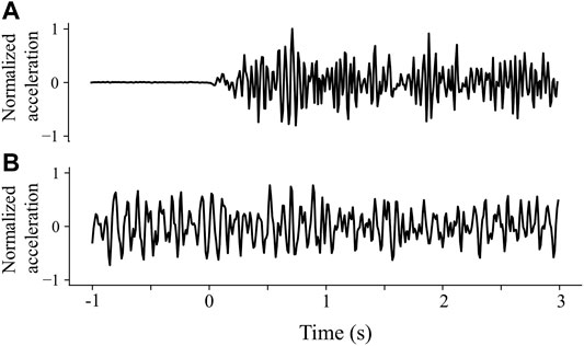
FIGURE 1. Examples of 4-s waveform data used in this study: (A) a P wave; (B) a microtremor. The point where the abscissa is 0 is the time of the P-wave arrival. The data in Figure 1 have been normalized.
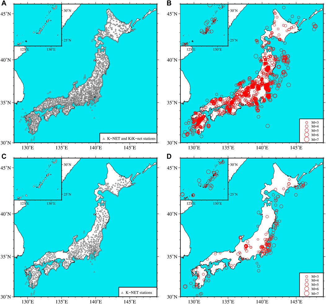
FIGURE 2. (A) Locations of the stations in the training set in this study. (B) Locations of the epicenters (open circles, size in proportion to magnitude) in the training set. (C) Locations of the stations in the testing set. (D) Locations of the epicenters in the testing set.
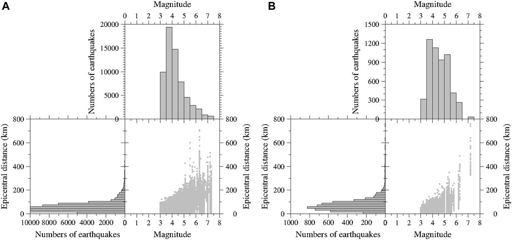
FIGURE 3. (A) Magnitude and epicentral distance distribution of the training set; (B) Magnitude and epicentral distance distribution of the testing set.
The testing set is different from the abovementioned data, which includes 7,774 K-NET vertical ground motion records throughout Japan from January 2020 to June 2020. All the data are complete waveforms with a sample rate of 100 Hz. The duration of most data is 120 s, and a small part is 60 s. After applying the same selection and preprocessing scheme, we obtain a testing set consisting of 5,373 P waves (Supplementary Table S2) and 5,373 microtremors. The locations of the corresponding stations and epicenters are shown in Figures 2C,D, respectively, and the magnitude and epicentral distance distributions are depicted in Figure 3B.
In addition, to verify the results of the combined model for practical applications, we chose the Great East Japan earthquake as an earthquake example, which occurred in the northeastern region of Japan on 11 March 2011 with a magnitude of 9.0 (Aoki et al., 2012). This earthquake was one of the largest earthquakes in Japan’s history. It caused substantial damage, killing tens of thousands of people and damaging hundreds of thousands of houses. Due to the large magnitude of this earthquake and the broad extent over which it was felt, researchers often use it as an earthquake example. We select 701 K-NET records and 525 KiK-net records during the earthquake, and the epicentral distances are from 120.83 to 1,336.74 km. After applying the same selection and preprocessing scheme for P waves, we obtain a testing dataset with 692 vertical-component records (Supplementary Table S3).
Materials and Methods
Training the Generative Adversarial Network
A GAN is an unsupervised ML algorithm proposed by Goodfellow et al. (2014); it consists of a generator (G) and a discriminator (D) (Goodfellow et al., 2014). Figure 4 shows the basic training process of a GAN. The black dotted line is the real data (

FIGURE 4. The basic GAN training process, which is reprinted with permission from Goodfellow et al. (2014). (A) The beginning of training GANs; (B,C) The training is in progress; (D) The end of training.
In this study, the flowchart depicting the training of a GAN is shown in Figure 5A. G takes the input of a 50-element vector drawn from a normal distribution and outputs a 4-s generated waveform (see the left box in Figure 5A). G is composed of two fully connected (FC) layers, in which there are 128 and 400 neurons. FC layers can map the distributed feature representation learned by a GAN to the space of sample labeling. In other words, the neurons in an FC can fit the distribution of real data, and the multilayer FC layers can solve the problem of nonlinear fitting. Every FC layer is followed by a leaky rectified linear unit (leaky ReLU), and the activation function of the last FC layer is given by a tanh function. Both tanh and leaky ReLU are activation functions. Because the output of neurons is the weighted sum of all inputs, the neural network is a linear model. The activation function increases the nonlinearity of the model; if the output of each neuron is passed through an activation function, the neural network can fit various distributions. The difference between the two layers is that a leaky ReLU is a nonsaturated activation function, which can effectively prevent problems such as gradient disappearance or gradient explosion, so it is often used in the hidden layer of neural networks. The output of tanh can be normalized to (-1, 1), which is convenient for input to D, so it is often used in the last layer. Additionally, we add a Reshape layer at the end of G to ensure that the generated data are acceptable for D. For D, the input is a 4-s waveform (either real data or generated data), and the output is the probability of the input waveform being a real record, as shown in the right box in Figure 5A. If the input waveform is from a real ground motion, the output is 1; if the input waveform is a generated waveform, the output is 0 (Li et al., 2018).
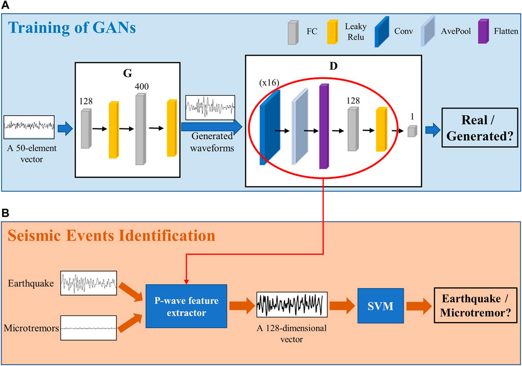
FIGURE 5. The training process of the combined model in this paper. (A) The training of GANs; (B) The identification of seismic events.
D consists of a convolutional (Conv) layer, an average pooling (AvePool) layer, and two FC layers. The Conv layer can extract waveform features through the forward propagation of convolution filters, which is the key to classification with D. Because forward propagation includes translation and flipping of convolution filters, it will produce a large number of training parameters. The AvePool layer can compress the input features, which not only simplifies the calculation complexity but also facilitates the extraction of the main features. The Conv layer has 16 filters, and the parameters of the other layers follow the default settings. The first FC layer has 128 neurons, followed by a leaky ReLU. The second FC layer has only 1 neuron to output the probability, and has a sigmoid activation function. The advantage of the sigmoid is that the output is between 0 and 1, which can serve as the probability of the output layer. Therefore, this function can not only predict the classification but also provide an approximate probability. We summarize these training settings in Table 1 and Table 2.
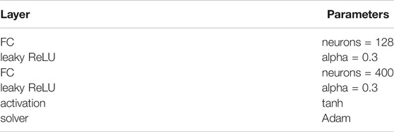
TABLE 1. Summary of the parameters of the G.
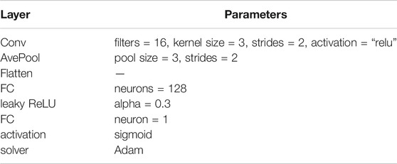
TABLE 2. Summary of the parameters of the D.
Moreover, we utilize Adam with learning rates of G and D of 0.0001 and 0.0002, respectively, thereby maintaining the balance of the data during training. Adam is a simple, computationally efficient, and low-memory optimizer that is used to update and calculate the parameters to minimize the loss function. In the training process of machine learning models, massive datasets often cannot be input into the model all at once, so researchers often input data in batches. In addition, it is usually not sufficient to train the model only once, and the epoch is the number of times the model is trained. In our study, training stopped when validation loss did not improve for 100 consecutive epochs and a batch size of 64; thus, G had 58,128 parameters and D had 203,073 parameters. These are all trainable parameters. Additionally, to achieve the purpose of classification, the loss functions of G and D are both binary cross entropy. We found that when D is trained for 5 iterations for each G iteration, the learning process achieves balance. These parameters are inherited from other GANs (Arjovsky et al., 2017) and are explored in this study to produce stable results. We select the model with the smallest validation loss as our final neural network model.
Identification of Seismic Events
Because the input of the GAN consists solely of real ground motions, the trained D can only distinguish between real data and generated waveforms. Therefore, we only use the GAN to extract P wave features and then use an SVM to identify P waves. An SVM is a binary classification model; its basic model is a linear classifier with the largest interval in the feature space (Webb, 2003). In other words, the principle of an SVM is to use a line or a manifold to divide various types, and the largest boundary is the optimal solution of the model. These characteristics make an SVM among the most powerful ML algorithms available today. When combined with a GAN, it can make full use of the P wave features extracted by the GAN for classification. Moreover, as the input to the SVM, microtremors can participate in the training of the combined model. Using the SVM as a classifier, rather than D itself, not only makes up for the shortcoming that microtremors cannot serve as input into the GAN but also leads to a much higher classification performance.
After the GAN training is complete, we remove the last FC layer of D and form the remaining part into a P-wave feature extractor, as shown in the red circle in Figure 5A. Assuming that after an extended period of training, D acquires the ability to distinguish real seismic waves, and the P-wave feature extractor serves to extract the key features of real earthquakes (Creswell et al., 2018). In this way, we can extract 105,074 waveform features, including 52,537 training P waves and 52,537 training microtremors, and input these into the SVM for classification, as shown in Figure 5B. It should be noted that the wave feature is a 128-dimensional vector. After the training of the SVM, the combined model can obtain the final classification results; that is, if the input is a P wave, the output is 1; if the input is a microtremor, the output is 0. We followed the initial settings in Scikit-learn for the training process of the SVM (Pedregosa et al., 2011). In addition, the parameter “model.predict_proba” of the Keras module in Python is used to provide an output probability (Pedregosa et al., 2011) serving to reflect the confidence in the decisions and thus assess the performance of the combined model.
Results
The Testing Set
After training, the well-trained model successfully identifies 5,359 P waves and 5,369 microtremors from the dual sample sets compromised of 5,373 records each. In other words, the combined model can achieve 99.74% accuracy for P waves and 99.93% accuracy for microtremors on the testing set. Table 3 shows the identification results, and Figure 6 shows examples of these four classifications, where the meanings of the four labels are as follows:
• A true positive indicates that a P wave is predicted to be a P wave.
• A true negative indicates that a microtremor is predicted to be a microtremor.
• A false positive indicates that a microtremor is mistaken as a P wave, which is a false alert in EEW.
• A false negative indicates that a P wave is mistaken as a microtremor, which is a missed alert in EEW.

TABLE 3. Identification of results on the testing set.
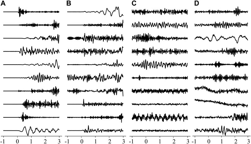
FIGURE 6. Examples of the 4 classifications. (A) True positive; (B) False negative; (C) True negative; (D) False positive. The point where the abscissa is 0 is the P-wave arrival. The data in Figure 6 have been normalized.
We can see that D is highly accurate for classifying P waves and microtremors. In Figure 6, the misclassified P waves generally have either relatively peculiar waveform shapes or nonsignificant onsets. In comparison, the misclassified microtremors have a relatively enduring wave train, which is similar to authentic P waves. Moreover, because the percentage of false positives in Table 3 is 0.07%, it is confirmed that this algorithm can effectively reduce the number of false alerts caused by microtremors. We go on to provide an output probability to analyze how confident the combined model is in the results. The output probability is a probability between 0 and 1, where 1 represents a P wave and 0 represents a microtremor. Therefore, the closer the output probability is to 1, the more likely it is that the testing data is a P wave. We count all the percentages of the test size with output probabilities in each interval (intervals are set to 0.1). Figure 7A shows the relationship between the output probabilities and the percentages of the testing data. The values at the two ends of the curves can evaluate the robustness of the identification ability of the algorithm. As shown in Figure 7A, 99.52% of microtremors and 99.37% of P waves in the testing set are concentrated on the two ends of the probability proxy, indicating that the combined model exhibits extremely high confidence in the results. Conventionally, probabilities of 0.1 and 0.9 are chosen as the decision boundary in this study; this threshold can be tuned at individual EEW stations (Li et al., 2018).
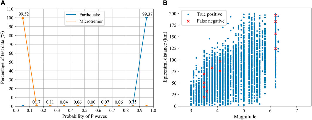
FIGURE 7. (A) The relationship between the percentage and output probability for the testing set. The earthquake data are concentrated in the 0.9–1.0 interval, and the microtremor data are concentrated in the 0–0.1 interval. Note that only half of the ordinate values are marked in the figure, including microtremor data with an output probability of 0–0.5 and seismic data with an output probability of 0.5–1.0. (B) The relationship between the epicentral distances and magnitudes of true positive records and false negative records with an epicentral distance ≤200 km for the testing set. The blue dots represent true positive records, and the red crosses represent false negative records.
Since most research on EEW is particularly interested in local earthquakes, we further analyze the discrimination performance for records whose epicentral distances are within 200 km, which is actually the distribution of true positives and false negatives on the epicentral distance. There are 5,373 P waves in the testing set; among them, 5,241 records have an epicentral distance of no more than 200 km. After training, 12 records are mistaken as microtremor signals. In other words, the proposed model can achieve 99.77% accuracy for local earthquakes. Figure 7B shows the relationship between the epicentral distances and magnitudes of the 12 mistaken records. The performance for small and medium earthquakes may be better than that for large events. Test data are more abundant for events with small magnitudes, but the mistaken waveforms are comparable to those of large earthquakes, indicating that the proposed model is more accurate in identifying small and medium earthquakes. This may be because the number of these earthquakes in the training set is relatively large, which gives the model more opportunities to extract features and make decisions.
To further explore the sensitivity of the combined model to different earthquake magnitudes, we next analyze the dependence of the identification performance on the magnitude, as shown in Figure 8A. The accuracy for all earthquakes is over 97%, and the performance for other magnitudes is surprisingly more than 99% except for those with
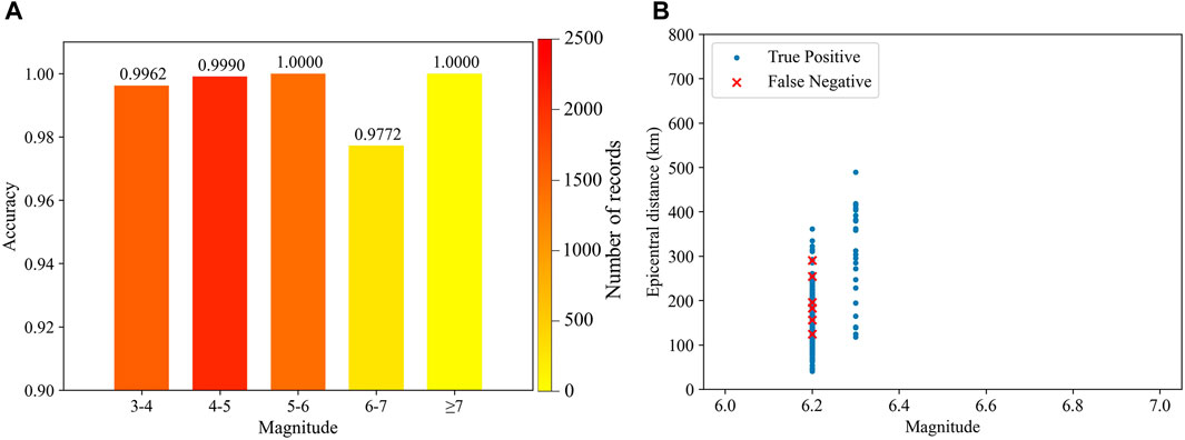
FIGURE 8. (A) Dependence of the performance on earthquake magnitudes. The colors of the columns are the number of test waveforms in the bins. (B) The relationship between the epicenter distances and magnitudes of earthquakes with
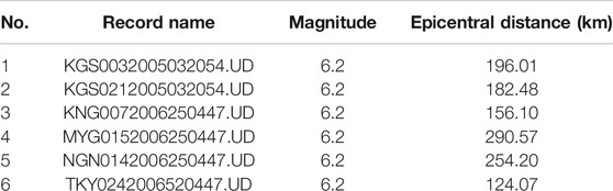
TABLE 4. Information about the misclassified earthquakes (false negative) for the testing set.
The Great East Earthquake
For the Great East earthquake, we input the dataset into the combined model and analyze the identification performance. Unfortunately, the well-trained model can only identify 287 records, corresponding to a considerably low accuracy of 41.47%. However, an examination of epicentral distances reveals that most misclassified waveforms are from regional stations (that is, epicentral distances over 200 km). Figure 9A shows the dependence of the identification performance on the epicentral distance, illustrating that the main reason why the accuracy is low is because of the poor performance for regional records; in contrast, the accuracy for local records (that is, epicentral distances within 200 km) is 98%. Therefore, for the purpose of EEW, we focus on analyzing the performance for local earthquakes. Among the 692 records in the dataset, only 50 records have an epicentral distance within 200 km. Figure 9B presents a schematic diagram of the discrimination results for these 50 records, revealing that only 1 local record is mistaken. Combined with Figure 9A, this finding demonstrates that although the overall performance of the proposed model drops considerably, the poor performance is predominantly due to regional records, whereas the performance for local stations is satisfactory. In other words, the proposed model can maintain perfect performance for local records during large events.
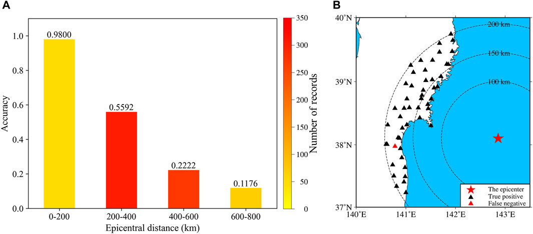
FIGURE 9. (A) Dependence of the combined model performance on the magnitudes for the Great East Japan earthquake dataset. (B) Locations of the true positive and false negative records with epicentral distances ≤200 km in the Great East Japan earthquake dataset. The red star represents the epicenter, and the triangles represent the locations of the triggered stations. Black indicates a true positive, and red indicates a false negative.
Comparison With the Short-Term Averaging/Long-Term Averaging Method
To highlight the superiority of this algorithm over traditional methods in identifying seismic events, we compare it with the STA/LTA method, which is currently the most widely used P-wave arrival picking algorithm. It is an energy method proposed by Allen (1978), which mainly uses the long-short-time ratio of the P-wave phase characteristic function to pick up the first arrival. The calculation formula used in this article is as follows.
Here, i is the sampling time. “Long” represents the length of the long-time window, “short” represents the length of the short time window, and λ is the trigger threshold. CF(j) is the P wave phase characteristic function (Allen, 1978; Allen, 1982), which characterizes the amplitude and energy changes of the data:
After P wave arrivals, the amplitude of the record will change greatly. This algorithm continuously calculates the average values of the absolute amplitude of a seismic signal in two consecutive moving-time windows. The short time window (STA) is sensitive to seismic events, while the long-time window (LTA) provides information about the temporal amplitude of the seismic noise at the site. When the ratio of both exceeds a preset value, an event is said to be “declared”; at this time, the data are recorded in a file (Trnkoczy, 2009). In this article, we used time windows of 0.5 and 30 s for the STA and LTA, respectively, and λ was set to 6. The parameters of the STA/LTA technique were selected to maximize the results.
Due to the relatively long-time window of 30 s, the calculation process of the STA/LTA method requires at least 30 s of ground motion records. As a result, we do not cut the input waveform for this method. In other words, we only perform the first three steps of preprocessing here. Moreover, this method does not require a training process, so we only need to input the test data into the STA/LTA method to obtain the final result. Because the output is the exact times of P-wave arrivals, not the results of the binary classification problem, we mark the result within 1 s before to 3 s after the actual P-wave arrival time as an earthquake identification success (that is, the output is 1). The remaining times are identification failures (that is, the output is 0).
Table 5 shows the comparison results of the two algorithms. Among 5,373 test earthquakes, the STA/LTA method can accurately identify 4,600 records. In other words, it can identify 85.61% of the test data. Compared with this traditional method, the combined model in this paper demonstrates a 14.13% increase in the identification accuracy of seismic events, indicating that our model is an accurate and reliable algorithm for seismic event identification. Nevertheless, due to the massive dataset, the combined model requires a long training and testing time, so it is slightly inferior to the STA/LTA method in terms of computational efficiency. In the future, we will continue to optimize the model to improve training efficiency and shorten the training and testing times.

TABLE 5. Comparison of the results with the STA/LTA method.
Discussion
With the goal of identifying seismic events from microtremors, we propose a new identification algorithm based on a combined ML model. We train a GAN based on 52,537 vertical strong ground motions from Japan and use a P-wave feature extractor to identify P waves from microtremors. After an SVM classifies the features to obtain a final result, we successfully transform the complex problem of identifying earthquakes into a simple binary classification problem of earthquakes and microtremors. The test results illustrate that the well-trained model can achieve accuracies of 99.74% for P waves and 99.93% for microtremors, which represents an improvement in accuracy of 14.13% compared with the traditional STA/LTA method. The results confirm that this algorithm can achieve state-of-the-art performance in discriminating between earthquakes and microtremors for EEW. Verification using a dataset from the Great East Japan earthquake indicates that the combined model can maintain a robust performance for local records at large magnitudes. Compared with manually labeling specific features associated with P waves, the algorithm can automatically extract the features that characterize P waves, thereby simplifying the training process and saving training costs.
Idea of Transformation
The main ideological innovation of this paper is to transform the identification procedure of seismic events into a binary classification problem between earthquakes and microtremors. The identification of seismic events is a very complex problem, and is made especially challenging due to a low SNR caused by the monitoring situation interfering with natural and anthropogenic seismicity activity, which can partially coincide in terms of magnitude, space, and time (Yang et al., 2021). However, ML methods can transform this issue into a binary classification problem. As a result, the combined model in this paper is confined to handling data in the feature space, which requires precise maneuvers and abundant field knowledge to construct a feature descriptor that can convert the raw data into a suitable representation. Subsequent machine learning then provides raw data for a model to automatically detect some unique features adopted for recognition. These approaches divide the identification process into two steps: 1) feature extraction and 2) classification. For our paper, although the GAN only uses a certain type of data as input, it can fully capture the statistical distribution of P waves, thereby automatically extracting those detailed features that can highly represent the data. In other words, the GAN can judge whether the data is a P wave. The SVM is a very practical binary classification model that can further purify the output of the GAN, thereby facilitating even more accurate judgments. Through this transformation, the problem of seismic event identification becomes simple and obvious and will not be affected by low SNRs. Consequently, the practicality of the algorithm has been enhanced, while the accuracy remains satisfactory.
Role of the Generative Adversarial Network and Support Vector Machine
A key purpose for using a GAN is to find an implicit or explicit representation of real data (Creswell et al., 2018). Specifically, the GAN captures the statistical distribution of P waves. D defines some form of similarity metric, and training narrows the gap between the generated and real data. Therefore, a well-trained GAN can grasp the key features of the real data. However, we did not directly use D to distinguish between P waves and microtremors because the microtremor data do not participate in the training of the GAN, and the classification results may not be convincing. Therefore, D is transformed into a P-wave feature extractor to extract specific patterns, which then allows for an SVM to identify seismic events. In this way, the microtremor data, which are part of the input to the SVM, also participate in the training process of the combined model. After a large amount of training, the SVM can automatically learn the differences in the waveform characteristics of the two types of data, allowing it to accurately distinguish between P waves and microtremor signals.
Performance on Specific Earthquakes
According to the performance of the model for local records and large earthquakes, it is evident that the combined model achieves a higher accuracy in identifying small and moderate earthquakes with magnitudes less than 6. One possible reason is that there is a high frequency of small and medium earthquakes, so the larger sample size helps the model extract features and make decisions. However, although the performance for large earthquakes is inferior to those of small and moderate magnitudes, it is still highly skillful. This could be caused by large earthquakes exhibiting longer-lasting waveforms and richer long-period components, so the combined model is still able to maintain high accuracy. Moreover, the results of local records are much more desirable than those of regional records, which coincides with EEW research. When we apply to the Great East Japan earthquake dataset, the performance is deemed sufficient for local records, indicating that the proposed algorithm is extremely robust for local stations.
Limitations
Although the proposed algorithm can accurately distinguish between earthquakes and microtremors, it still suffers from many shortcomings. First, the proposed algorithm pertains only to microtremors, and thus, further research must be performed to develop a method such as that of Li et al. (2018) that is capable of distinguishing between earthquakes and other types of noise. Second, the training of this algorithm is relatively complicated. Compared with other machine learning algorithms, such as convolutional neural network (CNN), it can only achieve the purpose of identifying seismic events. Hence, this algorithm needs to be combined with an automatic detection algorithm, such as Allen (1978), to accurately identify earthquakes. Integrating earthquake detection, localization, and characterization is our future work, such as Majstorović et al. (2021). Moreover, the dataset we used for this study is highly selective (only composed of strong ground motion and clean, pre-P microtremors), so this is a proof-of-concept test of machine learning for identifying P waves. The current training and testing times are long, further illustrating that the training efficiency needs to be improved. Finally, as a byproduct (Creswell et al., 2018), the simulated waveform generated by G participates in the internal loop of the training of the GAN and has not yet been specifically applied. We are not sure whether the generated waveform can truly reflect the characteristics of real earthquakes. We will continue to improve the combined model identification performance and data optimization, as we expect that the idea of transforming identification problems into binary classification can enjoy broad applications that are beyond the scope of this study.
Conclusion
In this study, we propose a new identification algorithm based on a combined model of a GAN and SVM, which transforms the complex problem of identifying earthquakes into a simple binary classification problem of earthquakes and microtremors. With the proper training parameters, our well-trained model can achieve accuracies of 99.74% for P waves and 99.93% for microtremors, which is an increase in accuracy of 14.13% compared with the traditional STA/LTA method, confirming that the proposed algorithm can achieve state-of-the-art performance for EEW seismic event identification. The results obtained for waveform records from the Great East Japan earthquake show that the proposed model can achieve a robust result for local records of large earthquakes. Hence, the proposed algorithm could have broad applications in EEW and earthquake monitoring.
Data Availability Statement
The original contributions presented in the study are included in the article/Supplementary Material, further inquiries can be directed to the corresponding author.
Author Contributions
HL implemented and applied the method and wrote the related text. JS contributed to designing the methodology and revised the manuscript. SL provided important suggestions for the interpretation of the results. All authors contributed to the redaction and final revision of the manuscript.
Funding
This research was financially supported by Scientific Research Fund of Institute of Engineering Mechanics, China Earthquake Administration (No. 2021B07), the National Key Research and Development Program of China (No. 2018YFC1504003), Natural Science Foundation of Heilongjiang Province (No. LH 2021E119), and the National Natural Science Foundation of China (Nos. 51408564, U1534202 and U2039209).
Conflict of Interest
The authors declare that the research was conducted in the absence of any commercial or financial relationships that could be construed as a potential conflict of interest.
Publisher’s Note
All claims expressed in this article are solely those of the authors and do not necessarily represent those of their affiliated organizations, or those of the publisher, the editors and the reviewers. Any product that may be evaluated in this article, or claim that may be made by its manufacturer, is not guaranteed or endorsed by the publisher.
Acknowledgments
We thank the National Research Institute for Earth Science and Disaster Prevention (NIED), Japan, for providing the K-NET and KiK-net station strong-motion data. Some plots were made using Generic Mapping Tools v.5.2.1 and the matplotlib module in Python.
Supplementary Material
The Supplementary Material for this article can be found online at: https://www.frontiersin.org/articles/10.3389/feart.2022.814655/full#supplementary-material
Supplementary Tables S1–S3 | Shows the seismic event information of the training set, the testing set and the Great East Earthquake used in this paper, respectively.
References
Allen, R. (1982). Automatic Phase Pickers: Their Present Use and Future Prospects. Bull. Seismol. Soc. Am. 72 (6B), S225–S242. doi:10.1785/BSSA07206B0225
Allen, R. V. (1978). Automatic Earthquake Recognition and Timing from Single Traces. Bull. Seismol. Soc. Am. 68 (5), 1521–1532. doi:10.1785/BSSA0680051521
Aoki, T., Fukumoto, Y., Yasuda, S., Sakata, Y., Ito, K., Takahashi, J., et al. (2012). The Great East Japan Earthquake Disaster and Cardiovascular Diseases. Eur. Heart J. 33 (22), 2796–2803. doi:10.1093/eurheartj/ehs288
Arjovsky, M., Chintala, S., and Bottou, L. (2017). “Wasserstein Generative Adversarial Networks,” in Proceedings of the International Conference on Machine Learning, Sydney, NSW, Australia, August 6–11, 2017 (USA: PMLR), 214–223.
Benz, H. M., McMahon, N. D., Aster, R. C., McNamara, D. E., and Harris, D. B. (2015). Hundreds of Earthquakes Per Day: The 2014 Guthrie, Oklahoma, Earthquake Sequence. Seismological Res. Lett. 86 (5), 1318–1325. doi:10.1785/0220150019
Brown, J. R., Beroza, G. C., and Shelly, D. R. (2008). An Autocorrelation Method to Detect Low Frequency Earthquakes within Tremor. Geophys. Res. Lett. 35 (16), L16305. doi:10.1029/2008GL034560
Creswell, A., White, T., Dumoulin, V., Arulkumaran, K., Sengupta, B., and Bharath, A. A. (2018). Generative Adversarial Networks: An Overview. IEEE Signal. Process. Mag. 35 (1), 53–65. doi:10.1109/MSP.2017.2765202
Goodfellow, I. J., Pouget-Abadie, J., Mirza, M., Xu, B., Warde-Farley, D., Ozair, S., et al. (2014). “Generative Adversarial Networks,” in Proceedings of the International Conference on Neural Information Processing Systems, Montrea, Canada, December 8–13, 2014 (Montreal, Canada: NIPS), 2672–2680.
Huang, Y., Zhang, S., Zhang, S., Lv, Y., Li, Y., Zhang, Y., et al. (2020). Earthquake Detection in the Jiangsu Region, China Using Graphics-Processing-Unit-Based Match & Locate and Rapid Earthquake Association and Location. Earthq. Sci. 33 (1), 23–33. doi:10.29382/eqs-2020-0023-03
Kong, Q., Allen, R. M., Schreier, L., and Kwon, Y.-W. (2016). MyShake: A Smartphone Seismic Network for Earthquake Early Warning and beyond. Sci. Adv. 2 (2), e1501055. doi:10.1126/sciadv.1501055
Li, Z., Meier, M.-A., Hauksson, E., Zhan, Z., and Andrews, J. (2018). Machine Learning Seismic Wave Discrimination: Application to Earthquake Early Warning. Geophys. Res. Lett. 45 (10), 4773–4779. doi:10.1029/2018GL077870
Majstorović, J., Giffard‐Roisin, S., and Poli, P. (2021). Designing Convolutional Neural Network Pipeline for Near‐Fault Earthquake Catalog Extension Using Single‐Station Waveforms. J. Geophys. Res. Solid Earth 126 (7), e2020JB021566. doi:10.1029/2020JB021566
Meier, M. A., Ross, Z. E., Ramachandran, A., Balakrishna, A., Nair, S., Kundzicz, P., et al. (2019). Reliable Real‐Time Seismic Signal/Noise Discrimination with Machine Learning. J. Geophys. Res. Solid Earth 124 (1), 788–800. doi:10.1029/2018JB016661
Mousavi, S. M., Ellsworth, W. L., Zhu, W., Chuang, L. Y., and Beroza, G. C. (2020). Earthquake Transformer-An Attentive Deep-Learning Model for Simultaneous Earthquake Detection and Phase Picking. Nat. Commun. 11 (1), 1–12. doi:10.1038/s41467-020-17591-w
Pedregosa, F., Varoquaux, G., Gramfort, A., Michel, V., Thirion, B., Grisel, O., et al. (2011). Scikit-learn: Machine Learning in Python. J. Mach. Learn. Res. 12, 2825–2830.
Peng, Z., and Zhao, P. (2009). Migration of Early Aftershocks Following the 2004 Parkfield Earthquake. Nat. Geosci 2 (12), 877–881. doi:10.1038/ngeo697
Ronneberger, O., Fischer, P., and Brox, T. (2015). “U-Net: Convolutional Networks for Biomedical Image Segmentation,” in Medical Image Computing and Computer-Assisted Intervention – MICCAI 2015. Editors N. Navab, J. Hornegger, W.M. Wells, and A.F. Frangi (Cham: Springer International Publishing), 234–241. doi:10.1007/978-3-319-24574-4_28
Ross, Z. E., Meier, M. A., Hauksson, E., and Heaton, T. H. (2018). Generalized Seismic Phase Detection with Deep Learning. Bull. Seismol. Soc. Am. 108 (5A), 2894–2901. doi:10.1785/0120180080
Saragiotis, C. D., Hadjileontiadis, L. J., and Panas, S. M. (2002). PAI-S/K: A Robust Automatic Seismic P Phase Arrival Identification Scheme. IEEE Trans. Geosci. Remote Sensing 40 (6), 1395–1404. doi:10.1109/TGRS.2002.800438
Sleeman, R., and Van Eck, T. (1999). Robust Automatic P-Phase Picking: An On-Line Implementation in the Analysis of Broadband Seismogram Recordings. Phys. Earth Planet. Inter. 113 (1-4), 265–275. doi:10.1016/S0031-9201(99)00007-2
Trnkoczy, A. (2009). “Understanding and Parameter Setting of STA/LTA Trigger Algorithm,” in New Manual of Seismological Observatory Practice (NMSOP). Editor P Bormann (Potsdam, Germany: Deutsches GeoForschungsZentrum GFZ), 1–20.
Yang, D.-H., Zhou, X., Wang, X.-Y., and Huang, J.-P. (2021). Mirco-Earthquake Source Depth Detection Using Machine Learning Techniques. Inf. Sci. 544, 325–342. doi:10.1016/j.ins.2020.07.045
Yoon, C. E., O’Reilly, O., Bergen, K. J., and Beroza, G. C. (2015). Earthquake Detection through Computationally Efficient Similarity Search. Sci. Adv. 1 (11), e1501057. doi:10.1126/sciadv.1501057
You, X., Yahong, D., Jia, H., Jiang, C., Zuofei, Y., and Wei, W. (2021). Microtremor-Based Analysis of the Dynamic Response Characteristics of Earth-Fissured Sites in the Datong basin, China. Earthq. Eng. Eng. Vib. 20 (3), 567–582. doi:10.1007/s11803-021-2039-2
Keywords: generative adversarial network, support vector machine, seismic event identification, earthquake early warning, classification
Citation: Liu H, Song J and Li S (2022) Seismic Event Identification Based on a Generative Adversarial Network and Support Vector Machine. Front. Earth Sci. 10:814655. doi: 10.3389/feart.2022.814655
Received: 14 November 2021; Accepted: 25 January 2022;
Published: 24 February 2022.
Edited by:
Faming Huang, Nanchang University, ChinaReviewed by:
Piero Poli, Université Grenoble Alpes, FranceAlexey Lyubushin, Institute of Physics of the Earth (RAS), Russia
Copyright © 2022 Liu, Song and Li. This is an open-access article distributed under the terms of the Creative Commons Attribution License (CC BY). The use, distribution or reproduction in other forums is permitted, provided the original author(s) and the copyright owner(s) are credited and that the original publication in this journal is cited, in accordance with accepted academic practice. No use, distribution or reproduction is permitted which does not comply with these terms.
*Correspondence: Shanyou Li, c2hhbnlvdUBpZW0uYWMuY24=