 Yongjian Yao
 Jian Zhang3*
 Miao Dong
 Hailing Liu
- 1Guangzhou Marine Geological Survey, Guangzhou, China
- 2Southern Marine Science and Engineering Guangdong Laboratory (Guangzhou), Guangzhou, China
- 3University of Chinese Academy of Sciences, Beijing, China
- 4Institute of Geology and Geophysics, Chinese Academy of Sciences, Beijing, China
- 5South China Sea Institute of Oceanology, Chinese Academy of Sciences, Guangzhou, China
The strike-slip fault system in the southwestern margin of South China Sea (SCS) lies on the transition zone between the continental shelf and slope of SCS, which is an important ocean–continent boundary. By using submarine heat flow data, a seismic shear wave tomography model, and gravity potential field data, this paper investigates the distribution of submarine heat flow in the southwestern margin of SCS, the thermal–rheological structure of the crust and mantle, the temperature–viscosity characteristics of the upper mantle Vs low-velocity layer, the tangential stress field of the rheological boundary layer at the lithosphere base, and the convective velocity structure of the mantle asthenosphere. Our new results show that the deep geothermal activity in the southwestern margin of SCS is intense, and the high heat flow area of the mantle with Qm/Qs >70% is distributed along an NNE-trending strip. Moreover, both the east and west sides of the strike–slip fault zone correspond to two low-value areas with a viscosity coefficient of 1021–1022 Pa⋅s at Moho depth, and beneath the Nansha Block are strong and cold blocks with a viscosity coefficient of 1024–1025 Pa⋅s. The northward and eastward shear stress components τN and τE of the rheological boundary layer at the base of the lithosphere mantle decrease with depth. At 65-km depth, both τN and τE are greater than 5.5 × 10⁸ N/m2. At 100-km depth, both τN and τE are less than 1 × 10⁸ N/m2. The calculation results based on the seismic shear wave model of the upper mantle and the gravimetric geoid model indicate that the depth of 120–250 km is the low-velocity layer, and the average temperature of the mantle at 180-km depth can be up to 1,300°C. Moreover, the average effective viscosity coefficient is close to 1018 Pa⋅s, which satisfies the temperature and viscosity conditions for partial melting or convective migration of mantle material. The mantle convection calculation results show that the average flow rate is 8.5 cm/a at 200-km depth and 2.2 cm/a at 400-km depth.
Introduction
The southwestern margin of South China Sea (SMSCS) lies on the transition zone from continental shelf to continental slope (Ding and Li, 2016; Dong et al., 2020), with direct geodynamic effect from the extrusion of Indosinia Block. It is the key region of plate convergence within the great circular subduction system of Southeast Asia (Lu et al., 2016) and also marks the tectonic termination where the oceanic crust of South China Sea (SCS) advances from east to west during “plate-edge rifting” (Wang et al., 2019). The southwestern margin of SCS is undergoing structural interactions between the strike–slip faulting and tectonic extrusion; thus, it has the most complicated tectonic elements but the lowest degree of geodynamic study in the periphery of SCS (Tapponnier et al., 1986; Yao et al., 1994; Liu, 1999; Ren and Li, 2000; Li et al., 2006; Li et al., 2012; Xu et al., 2016). Over the last decades or so, there are two major geodynamic questions that remain to be answered. The first is as follows: during the southward propagation of the strike–slip fault zone in the SMSCS, is there any continuity or connection between the Zhongjian Fault, Wanan Fault, Lupar Fault, and Tinja Fault? The second is also as follows: during the tectonic extrusion of the Indosinian Peninsula, the circular subduction of Southeast Asia, and the rifting-expansion of SCS, how do the tectonic forces interact with each other during different periods and at various directions?
These two major questions have been subjected to intensive study in association with the geodynamic history of SCS (Yao et al., 2004; Liu et al., 2015; Sun et al., 2006; Fyhn et al., 2009). It is necessary to “observe the SCS by stepping out of the SCS” and “observe the SCS by going deep into the SCS”. Substantial data and results have been obtained after many years of marine scientific research in SCS (Li et al., 2010; Xu et al., 2016; Xu et al., 2016; Dong et al., 2018). Since the 1980s, especially Guangzhou Marine Geological Survey has carried out a series of comprehensive geological and geophysical surveys on “oil and gas resources” and obtained significant gravity, magnetic, seismic, and heat flow data. In recent years, the Program for Marine Basic Geological Survey has enriched the geological understanding of the southwestern margin of SCS. With measured submarine heat flow data at the southwestern end of the Southwest Basin in the SCS (Xu et al., 2005; Li et al., 2010; Xu et al., 2016; Dong et al., 2018) and based on seismic and gravity data, this paper analyzes the thermal structure of the crust in the southwestern margin of the SCS, the rheological characteristics of the base of the lithospheric mantle, and the geodynamic background of the deep convective mantle, providing a reference for studying of the region and having important significance for understanding of the dynamic model of seafloor spreading of the SCS and reconstruction of the Asian tectonic framework in the geodynamic process and deep material circulation, tectonic deformation and dynamic mechanism.
Geodynamic Background
The study area is located at the center of the curved convergent system in Southeast Asia (Figure 1A). Seismological studies (Huang and Zhao, 2006; Zhao and Ohtani, 2009) indicate that the oceanic slabs on both the east and west sides of the annular subduction belt in Southeast Asia present opposite subduction directions (Fukao et al., 1992), which form a convergent system of subduction fronts with different depths and origins in three directions, i.e., east, west, and south. The convergence of multi-directional subduction slabs affects the circulation of deep mantle material, thermal-viscosity structure, and rheological property.
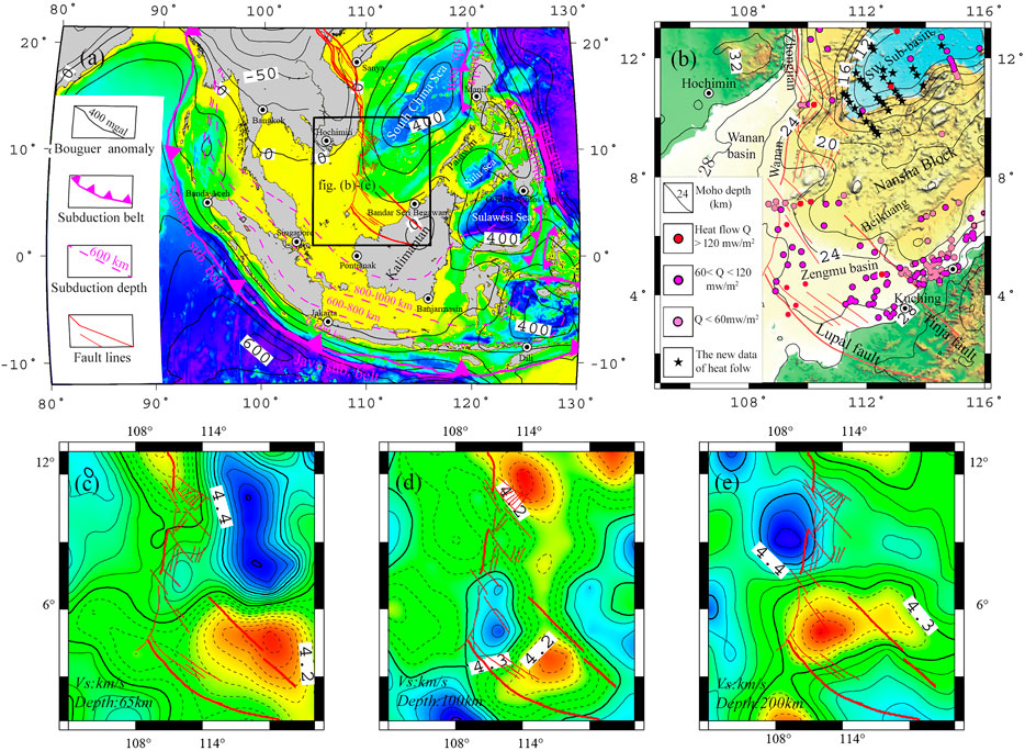
FIGURE 1. Regional map of the southwestern margin of South China Sea (SCS). (A) Tectonic map of the southwestern margin of SCS. (B) Map of the geothermal geology in the study area. (C–E) Vs map at depths of 65, 100, and 200 km (Chen et al., 2021).
Geology Setting
The southwestern margin of SCS (Figure 1B) represents the extensional area of the Southwest Basin in the SCS. It is bound by the Indosinian Peninsula in the northwest and by Kalimantan Island in the southeast, respectively. The fault zone in the western margin of SCS runs southward through the study area from the east side of the Indosinian Peninsula and then bends toward southeast into Kalimantan Island. It marks the western boundary of SCS and is primarily deformed by strike–slip faulting (Fyhn et al., 2009; Lin et al., 2009; Gao, 2011; Xu et al., 2016). Overall, the strike–slip fault zone is composed of a series of faults that trend roughly NNW–SSE. Its north termination starts from the Yinggehai Sea with connection to the Red River Fault and Yinggehai Fault. Towards the south, the fault zone comprises the Zhongjian Fault, Wanan Fault, Lupal Fault, and Tinja Fault. Moreover, the south termination runs deep into Borneo Island. In the study area, Zhongjiannan Basin, Wanan Basin, Nanweixi Basin, and Zengmu Basin are developed along this strike–slip fault zone (Zhan et al., 1995; An et al., 2012; Yao et al., 2013). Geomorphologically, the strike–slip fault zone is situated at the transition from the continental shelf to the slope in the west SCS; as such, the topographic and geomorphic features on both sides of the fault zone appear to be quite different. In the west side, the water depth at the outer shelf edge is 200–250 m, and the shelf itself is narrow, with a topographic slope of 10–22°. The landform from Da Nang to the south of Ho Chi Minh City in Vietnam is relatively broad and flat, with a topographic slope of 4.7°. In the east side, the continental slope has a water depth ranging between 200 and 4,000 m. The topography is complicated with distinct variations. From north to south, there are Xisha Trough, Xisha Islands, Zhongsha Islands, West Basin Ridge, West Basin Canyon, Southwest Basin Ridge, etc., with a topographic slope of 6.7–17.6°.
Since the Cenozoic period, the strike‐slip fault zone in the western margin of SCS has evolved into three distinct segments in the upper crust from north to south, i.e., the Ailaoshan-Honghe fault zone, the Yinggehai‐Zhongjian fault zone, and the Wanna‐Lupal fault zone. Spatially, these strike-slip fault zones show different sense of movements, such as left‐lateral slip and right‐lateral slip. Despite of this, these faults are geodynamically governed by the southeastward intrusion of the Indo‐China block induced by the collision between the Indian plate and the Eurasian plate, as well as the seafloor spreading of SCS (Liu et al., 2015).
Characteristics of Gravity Field
In the regional gravity Bouguer anomaly map (Figure 1A), it can be seen that the east, south, and west sides of the study area are dominated by high Bouguer anomaly with a value of up to 600 mgal, while the north side is characterized by low continental Bouguer gravity anomaly, with a value of ≤50 mgal. The strike–slip fault zone is marked by the boundary between the low gravity of the Indosinian Peninsula and the high gravity of SCS. For this gravity anomaly transition zone, the fault strike, dip, and slip can be estimated through a calculation of the change rate of the gravity gradient. Taken together, the gravity inversion results show (Figure 1B) that the overall Moho depth in the study area ranges between 8 and 32 km (Zhang et al., 2017). Specifically, the Indosinian Peninsula in the northwest and Kalimantan Island in the southeast belong to the continental crust whose Moho surface is deep, i.e., maximum of 32 km. In contrast, the Southwest Basin of SCS is part of the oceanic crust whose Moho is shallow, with a minimum value of 10 km. The rest of the area represents the geomorphic transition area. Its Moho depth appears to become deeper along the axis of the Southwest Basin at 16–28 km, forming a “mirror reflection” with the submarine topography.
Characteristics of Submarine Heat Flow
The submarine heat flow contains information such as the thermal state of the oceanic crust and the mantle as well as the thermal structure of the lithosphere, which lays the foundation for the dynamic analysis of marine geological structures. Many research progresses have been made in studying the submarine heat flow and its characteristics in SCS (Qian, 1992; Yao et al., 1994; Nissen et al., 1995; Shi et al., 2003; Xu et al., 2005; Li et al., 2010). With the advancement of basic marine geological survey and exploration of deep-water oil and gas and natural gas hydrate resources, the total number of submarine heat flow data in the SCS has exceeded 1,250. The submarine heat flow measurement sites in SCS are mainly located on the southern and northern continental margins of the SCS, and the data obtained from temperature measurement in oil drilling sites on the continental shelf are more than that taken from the submarine probes. According to a statistical analysis (Zhang and Wang, 2000), about 42.6% of heat flow data came from the southern margin of the SCS, with an average value of 80.8 mW/m2. The southern SCS can be divided into the east and west heat flow regions by the Beikuang-Tinja Fault, which correspond to the low-heat-flow region of Nansha Islands and the high-heat-flow region of Zengmu Basin, respectively. Due to the irregular distribution of heat flow measurement sites, especially the scarcity of heat flow data along the strike–slip fault zone, the reef area on Nansha Islands and Nansha Trough, an in-depth analysis of geothermal field and thermal state on the western margin of the SCS has been largely inhibited.
From 2015 to 2018, during the oceanic expedition of “Marine, 4th” HY4201508 of Guangzhou Marine Geological Survey, an additional 30 new submarine heat flow datasets were obtained in the southwest sub-basin of the SCS (Xu et al., 2016; Dong et al., 2018). The geographic range of the measurement sites of these data is between 112°22′43″–114°31′47″ E and 9°26′29″–12°24′01″ N (Figure 1B). The variation range of the thermal conductivity of sediments at the 30 measurement sites is at 0.77–1.07 W/(m⋅K), with an average of 0.86 W/(m⋅K). Based on the content of uranium, thorium, and potassium from 13 survey sites, the range of heat production rate is calculated to be 0.78–1.41 μW/m3, with an average value of 1.12 μW/m3. Thus, the distribution of the submarine heat flow at each survey site is estimated to be 75.9–126.1 mW/m2, with an average value of 94.1 mW/m2. The combined newly acquired and previously existing submarine heat flow data is able to well reflect the temporal and spatial distribution of the current geothermal field and deep thermal state in this study area.
Deep S Wave Velocity Characteristics
A recent study proposed the new generation of high-resolution 3D shear wave velocity model for SCS (Chen et al., 2021). The model presents 3D shear wave velocities across the SCS and its adjacent areas at the depth ranging between 15 and 250 km by joint inversion of ambient noise and surface wave dispersion. It has a high resolution of the crust–mantle structure and can provide accurate seismic wave depth anomalies. Therefore, the latest marine shear wave model is suitable for a deep dynamic analysis of the SCS.
Figures 1C,D,E are the 3D shear wave velocity model slices at 65-, 100-, and 200-km depth, respectively. At 65-km depth (Figure 1C), the tectonic characteristics of the SCS Basin gradually diminishes, while the characteristics of the strike–slip fault zone in the western margin of the SCS increasingly becomes obvious. Moreover, a low-velocity region consistent with the strike–slip fault is observed. The Zengmu Basin in the southwestern margin of the SCS shows a low Vs anomaly of ≤4.2 km/S, indicative of the upwelling of asthenospheric material, whereas the Nansha Block presents a high Vs anomaly of ≥4.4 km/S, suggesting the presence of cold strong blocks. At 100-km depth (Figure 1D), the N–S-trending low-velocity anomaly zone from the Zhongjiannan Basin to the Zengmu Basin is very obvious, implicating the existence of a low-velocity weak region in the upper mantle. The NW–NS–NE clockwise rotation gradually becomes distinct, which coincides with the clockwise rotation during the sinistral movement of the Indosinian Peninsula relative to the South China Block since Mesozoic. At 200-km depth (Figure 1E), the characteristics of the strike–slip fault appears to be gone, reflecting the material migration in the mantle asthenosphere and the deep dynamic process, whereas the Zengmu Basin still shows a low Vs anomaly, indicating that the upwelling channel of the deep asthenosphere material in the Zengmu Basin has the characteristics of continuity, which supports the continuous partial melting of the asthenosphere; however, a significant high-velocity anomaly of ≥4.4 km/S is observed beneath the Wanan Basin, indicating that the lithosphere base is cold and thick and might have to be squeezed into a rigid block during the strike–slip faulting. It reflects the dynamic evolution of the East Asian continental margin due to the subduction of the Pacific Plate as well as the great shear extrusion of the Tibet Plateau.
Deep Thermal-Dynamic Structure Model and Calculation Method
Crust–Mantle Thermal Structure Model
Global seismological observations and studies showed that there is a low-velocity seismic layer caused by partial melting of the mantle material at 60-km depth beneath the sea or at 120- to 250-km depth beneath the continent, and the partially molten mantle material in the layer has formed a slow-flowing asthenosphere in a semi-viscous state. The mantle convection studies indicated (Doin et al., 1997; Dixon et al., 2004; Paulson et al., 2010) that there is a rheological boundary layer (RBL) with a certain thickness between the solid lithosphere (crust and solid mantle) and the fluid mantle. Above the RBL is the solid lithosphere dominated by heat conduction, beneath the RBL is the upper mantle asthenosphere dominated by thermal convection, and between the lithospheric mantle and the asthenospheric mantle is a RBL where heat conduction and heat convection coexist. Figure 2 shows the theoretical geothermal line (conduction geothermic), the melting temperature line of mantle material (peridotite solidus), and the adiabatic compression temperature line (adiabat) of mantle material calculated based on the one-dimensional Fourier heat conduction equation. The three lines meet at a depth of 120–250 km, which is the partial melting zone of the mantle material. The location of the seismic low-velocity layer in the southwestern margin of the SCS roughly corresponds to the partial melting depth zone of mantle material (Figure 2). Based on this, it can be inferred that there is material convection or migration activity at this depth range. Considering that the temperature and pressure state of the upper mantle material is close to the adiabatic compression process, the mantle convection may actually involve thicker layers, and the lower boundary can extend to 440 km.
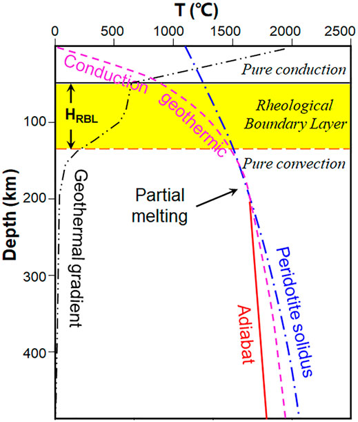
FIGURE 2. Diagram of the crust–mantle thermal structure model.
Calculation Method
(1) Calculation method for crust and upper mantle temperature
The method of solving the steady-state heat conduction equation is mainly used for the calculation of crust temperature. The steady-state heat conduction equation can be expressed as:
In Eq. 1, the distribution of temperature T depends on the heat production rate A and thermal conductivity K, and its parameter range is shown in Table 1.

TABLE 1. Thermophysical property parameters (Zhang et al., 2005; Meng and Zhang, 2014).
In real calculation, the steady-state conduction temperature field is obtained, while factors such as the unsteady-state lateral heat transfer caused by the submarine shallow structure are not taken into account.
The upper mantle lacks thermal constraints, and the rheological state does not meet the conditions of steady-state heat conduction, so the steady-state heat conduction equation cannot be used to calculate the mantle temperature. The upper mantle temperature can be calculated by using the relation between shear wave Vs inelastic component and temperature T and pressure P. In the depth range of 50–250 km, the lithological inelasticity is mainly affected by temperature, which is the main factor for controlling the seismic wave velocity (Sobolev et al., 1996; Goes et al., 2000; An and Shi, 2007). Under high temperature conditions, by means of inelastic correction of the quality factor Q, the calculation formula of temperature-dependent Vs wave velocity after inelastic correction can be obtained as follows:
In Eq. 2, A and a are inelastic constants, ω is inelastic effect frequency, E is activation energy, V is activation volume, and R is gas constant.
In real calculation, it is considered that, within the depth range of 50–250 km, the change of wave velocity caused by mineral composition is small, but the change of wave velocity caused by temperature is relatively large. If the shear wave velocity structure at each depth of the upper mantle is known, the difference value of ΔVs between the wave velocity and the observed wave velocity can be calculated through iterative inversion under given initial conditions, and the initial temperature model can be continuously corrected to decrease ΔVs (less than 0.1%) to obtain the 3D temperature field distribution of the mantle.
With the VS wave velocity model and the calculated temperature, the viscous structure of the crust–mantle material can be calculated by the following formula:
In Eq. 3, η is viscosity coefficient, E is activation energy, λ is adjustment coefficient, α is coefficient of thermal expansion, R is gas constant, and T is Kelvin temperature.
(2) Calculation method for shear stress field of the rheological layer of the crust and mantle
Deformation is the result of diffusion and transfer of viscous materials. This diffusion is carried out by means of pressure melting (pressure solution). Under the action of bearing deviatoric stress or tectonic stress, the rocks in the deformation region transfer the material from the high-intergranular-pressure-and-stress region to the low-pressure-and-stress region, resulting in creep. Both dislocation creep and diffusion creep can realize the “plastic” flow of solid matter. The dislocation (or power law) creep stress index n ≈ 2.5–3.5, and the diffusion creep n = 1. Laboratory studies support the dislocation creep at the shallow upper mantle (Turcotte, 2014). According to the spherical harmonic function coefficients Cnm and Snm provided by the satellite gravity and the spherical function Pnm, the shear stress field τ at different depths of the lithosphere can be calculated (Runcorn, 1964; Runcorn, 967) with the following formula:
In Eq. 4, U is the gravitational disturbance potential calculated based on Molodensky theory, σN and σE are north and east shear stress components generated by the rheological layer on the lithosphere base.
In actual calculation, the relation between the spherical harmonic order n at any point and the mass buried depth Dn at the corresponding equivalent point is taken as (Bowin, 1983) Dn = R / (n - 1), where R is 6,371 m.
(3) Calculation method for the flow field of asthenospheric mantle material
Supposedly the temperature variation only affects the density of asthenospheric material, and then this density change may lead to convective activity. The thermal convection equation that describes this density change is as follows:
In Eq. 5, V is convective velocity, P is pressure, g is gravity, η is viscosity coefficient, ρ is density, κ is thermal diffusion coefficient, A is heat production rate, c is constant pressure specific heat, T is temperature, and α is coefficient of thermal expansion.
In real calculation, the asthenosphere will be considered as a kind of high-viscosity fluid movement on a geological time scale. Viscosity is an important factor for controlling the viscous flow of the mantle. With the depth-dependent viscosity and seismic shear wave velocity Vs obtained by simulating the geoid height anomaly, the flow field of the asthenospheric mantle can be solved.
Crustal Thermal–Rheological Structure and Upper Mantle Dynamics
Crustal Temperature and Viscosity
The submarine heat flow distribution (Figure 3A) drawn by Kriging interpolation using the new heat flow data (indicated with black five-pointed stars) and the existing heat flow data (indicated with red and blue circles) show that the submarine heat flow Qs in the study area shows an obvious NNE-trending strip-shaped distribution pattern. Along the axis of the Southwest Basin, the SSW-trending and strip-shaped high-value heat flow anomaly is observed. At the north and south terminations of the high heat flow strip, there are high heat flow areas in the Southwest Basin and the Zengmu Basin, respectively. On the east side of the high heat flow, a low heat flow anomaly is seen on the Nansha Block, while on its west side a high-value heat flow anomaly area is observed in the Wanan Basin.
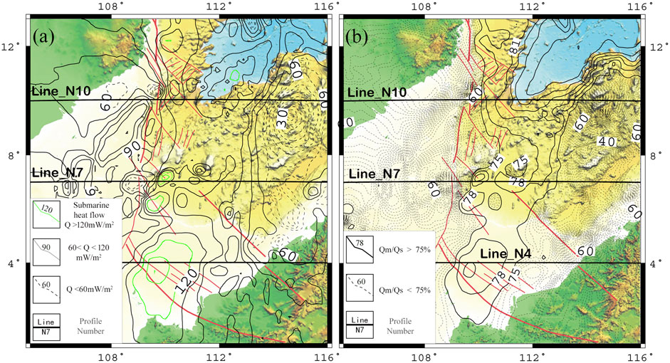
FIGURE 3. Contour maps of the submarine heat flow and the Qm/Qs heat flow structure in the southwestern margin of South China Sea. (A) Submarine heat flow Qs: mW/m2. (B) Qm/Qs: %.
The submarine heat flow Qs is equal to the sum of the crustal heat flow Qc and the mantle heat flow Qm, and the ratio of the crust and mantle components Qm/Qs of the submarine heat flow is an important parameter for studying the heat flow distribution of the crust and the mantle. With the submarine heat flow data Qs (Figure 3A), the Moho depth obtained by gravity inversion, and the heat production rate (Table 1), the calculated Qm/Qs results (Figure 3B) indicate that the NNE-trending strip-shaped distribution pattern of Qm/Qs is very clear, and the area with Qm/Qs >70% shows a distinct strip shape, which extends to the southwest region along the axis of the Southwest Basin. The Qm/Qs on both the east and west sides of the strip is less than 60%, and the Qm/Qs in the local area is less than 40%. This crust–mantle heat flow ratio indicates that the heat from the mantle is much higher than that of the crust from the Southwest Basin to the Zengmu Basin, and it is a “hot mantle” zone. On both sides of this strip, especially in the Nansha Block, the mantle heat is relatively low, and it is a “cold mantle” zone.
After de-peaking to the submarine heat flow data in the study area (Figure 3A) (Qs >140 mW/m2, 140 mW/m2 is taken; Qs <40 mW/m2, and 40 mW/m2 is taken, in order to eliminate the non-conductive heat effect caused by hydrothermal activity), the steady-state heat conduction equation is solved with the crust–mantle structure of gravity inversion and thermophysical parameters (Table 1) (Zhang et al., 2005), and the temperature results of the profiles at N10°, N7°, and N4° (the location of the profiles is shown in Figure 3) are shown in Figures 4A–C. The results of the profile viscosity calculated from the temperature distribution and the Vs wave velocity distribution are shown in Figures 4D–F.
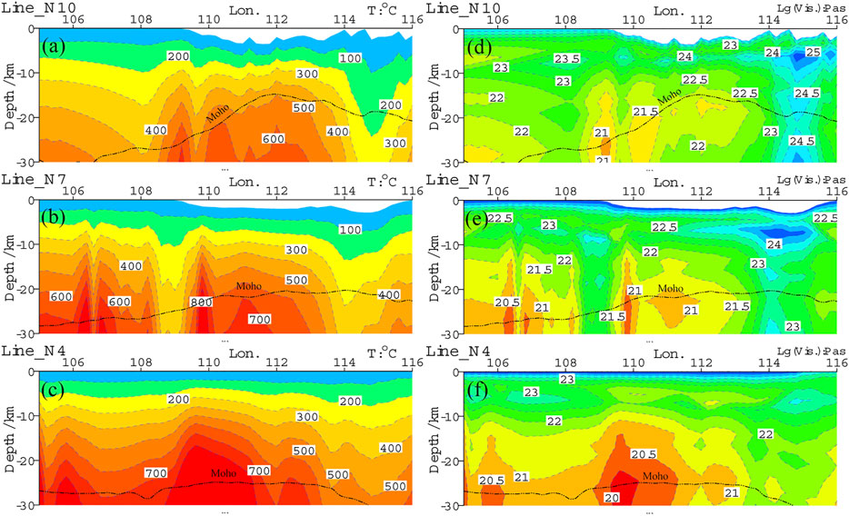
FIGURE 4. Temperature and viscosity coefficient profiles in the southwestern margin of South China Sea. (A–C) Temperature profiles at Line_N10, Line_N7, and Line_N4. (D–F) Viscosity coefficient profiles at Line_N10, Line_N7, and Line_N4. The position of the profiles is shown in Figure 3, and the earth surface is the starting point of depth.
The starting point for the depth of each profile (Figure 4) is the sea level, of which on the profile at N10° (Figure 4A), E108°, and E115°, there are two low-temperature zones at depth, with Moho temperatures of 390 and 180°C, respectively. However, high-temperature zones appear on the east and west sides of the strike–slip fault zone (at E110°), and the Moho temperature is higher than 600°C. Beneath the corresponding strike–slip fault zone, the Moho temperature is lower than 500°C. On the profile at N7° (Figure 4B), a clear low-temperature zone appears at E109°, which corresponds to the intersection area of the strike–slip zones in the southeastern margin of Wanan Basin, and in the western margin, the Moho temperature is lower than 350°C. To the east of E114°, there is also a low-temperature zone, with the Moho temperature being lower than 300°C. The low-temperature zone on the east side corresponds to the Nansha Block and Nansha Trough, which is caused by the abnormal cooling of the mantle (Zhang et al., 2017). On the profile at N4° (Figure 4C), the temperature distribution has changed significantly. This profile corresponds to the Lupal Fault Zone and the Tinja Fault Zone in which the strike–slip fault zone in the western margin bends to the southeast. The deep geothermal activity caused by tectonic activity is intense, and the Moho temperature is significantly higher than that of the N10° profile and N7° profile on the north side, of which the Moho temperature in the Zengmu Basin at E110° is as high as 900°C.
With the temperature profiles (Figures 4A–C) and based on the 3D shear wave velocity structure (Chen et al., 2021), the calculated viscosity coefficient profiles are shown in Figures 4D–F, of which on the profile at N10° (Figure 4D), at Moho depth on the east and west sides beneath the strike–slip fault zone in the western margin, these are characterized by two low-viscosity-coefficient regions, with a viscosity coefficient at 1021–1022 Pa⋅s. Beneath the Nansha Block is a high-viscosity-coefficient region that is vertically extended, with a viscosity coefficient at 1024–1025Pa⋅s. On the profile at N7° (Figure 4E), on both the east and west sides of the strike–slip fault zone are two separate low-viscosity-coefficient regions, but their separation distance is larger than that of the north side, and the viscosity coefficient on the east side is much lower, which can be as low as 1020 Pa⋅s at 110°C. However, the vertically extended high-viscosity-coefficient region beneath the Nansha Block shrinks upward, forming a “hard core” with a viscosity coefficient of greater than 1024 Pa⋅s at a depth of 5–10 km. On the profile at N4° (Figure 4F), due to the increase in temperature, the viscosity coefficient near the Moho surface is low, and a “weak rheological zone” with a viscosity coefficient of less than 1020 Pa⋅s is formed near the Moho surface, and partial melting may exist.
Upper Mantle Dynamics
Thermal–rheological analysis of gravity and seismic data is an important method for deep dynamic study. The comprehensive analyses of the gravity field EGM2008 model, the satellite gravity data, and the seismic shear wave model (Chen et al., 2021) indicated that, at 40-km depth or beneath the Moho in the southwestern margin of SCS, the influence of the tectonics of the SCS Basin is gradually decreasing, and the characteristics of the strike–slip structure in the western margin is becoming progressively clear; at 70-km depth or below, a low-velocity uplift consistent with the strike–slip structure trend is observed; at 100-km depth or below, the characteristics of the strike–slip structure in the western margin of the SCS are gradually weakening, and the NW–NS–NE clockwise rotation effect steadily becomes prominent, which coincides with the clockwise rotation during the sinistral movement of the Indosinian Peninsula relative to the South China Block after the Mesozoic; at 200-km depth or below, the clockwise rotation effect is gradually weakening, and the NE-trending structure becomes more obvious.
According to the crust–mantle thermal structure model given in Figure 2, there is a RBL in a specific thickness interval at the lithosphere base. The rheological boundary layer can transfer the tangential stress generated by the mantle flow to the lithosphere to form a lithospheric stress and to deform the lithosphere. If it is assumed that there is a Newtonian viscous laminar flow beneath the rheological boundary layer and an elastic lithosphere above the rheological boundary layer, then an equilibrium equation at r = r′ on the upper boundary of the mantle flow is constructed by the gravitational disturbance potential generated by Navier–Stokes equation and uneven density. Suppose the radial component of the velocity at r = r′ is zero. In this case, equilibrium equation can be solved with this equilibrium equation and the spherical harmonic function of the gravitational potential to obtain the north and east shear stress components at different depths in the rheological boundary layer τN, τE (Runcorn, 1964; Runcorn, 1967; Bowin, 1983; Wu and Liu, 1992; Fu et al., 1994). The depth at the lithosphere base fluctuates, and the thickness of the rheological layer is uneven. The stress distribution at a depth of 65 and 100 km in the study area (Figure 5) is calculated with Eq. 4.
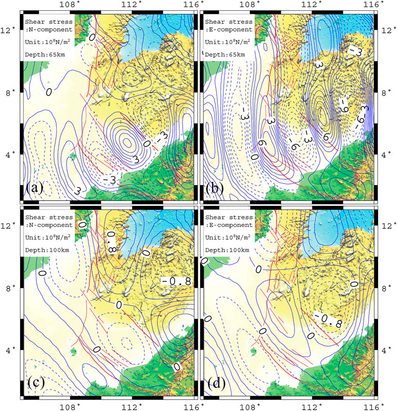
FIGURE 5. Stress field at the rheological boundary of the upper mantle in the southwestern margin of South China Sea. (A) Northward shear stress τN at 65-km depth. (B) Eastward shear stress τE at 65-km depth. (C) Northward shear stress τN at 100-km depth. (D) Eastward shear stress τE at 100-km depth. τN—positive in the north and negative in the south; τE—positive in the east and negative in the west.
The southwestern margin of the SCS has experienced intense shear deformation and tectonic extrusion caused by the subduction of the Pacific Plate in the Mesozoic as well as the creeping, rifting, and drifting of the South China continent towards the southeast along with mantle convection, which left traces in the upper mantle. Therefore, an analysis can be carried out with the northward shear stress component τN and the eastward shear stress component τE at the depth of 65 and 100 km in the rheological boundary layer calculated from the gravity potential data (Figure 5). The northward shear stress component τN at 65-km depth in the rheological boundary layer is −5.78–6.32 × 10⁸ N/m2 (Figure 5A). In the middle section of the strike–slip fault zone, τN is a “positive” value, whereas in the southern part of the strike–slip fault zone, the Zengmu Basin between the Lupal Fault Zone and Tinja Fault Zone is an NW-trending strip zone where τN is characterized by alternation of “positive” and “negative” values. The eastward shear stress component τE at 65-km depth in the rheological boundary layer of this area is at −11.09–8.66 × 10⁸ N/m2 (Figure 5B). Overall, τE is distributed alternately in a long S–N-trending strip from west to east. The eastward shear stress component τE is a “positive” value zone on the west side of the strike–slip fault zone and a “negative” value zone on the east side. The northward shear stress component τN at 100-km depth in the rheological boundary layer of the study area is at −1–1 × 10⁸ N/m2 (Figure 5C). The Zengmu Basin between the Lupal Fault Zone and the Tinja Fault Zone in the southern section of the strike–slip fault is a “negative” low-value shear stress zone, and this “negative” value area forms a long-axis NW–SE-trending ellipse. The “negative” stress zone in Zengmu Basin extends toward the northwest. After crossing the middle section of the strike–slip fault zone in the western margin, it forms a “negative” value zone in the long axis near the N–S-trending ellipse on the north side of Wanan Basin. This “negative” value zone and the “positive” value zone in the long axis near the NS-trending ellipse in Zhongjiannan Basin are distributed in parallel to each other in the west and east of the middle section of the strike–slip fault zone, forming a southward shear zone on the west side and a northward shear zone on the east side. The eastward shear stress component τE at 100 km depth in the rheological boundary layer of this area is at −1∼1 × 10⁸ N/m2 (Figure 5D). At this depth, the southern section of the strike–slip fault zone in the western margin and Zengmu Basin between the Lupal Fault Zone and Tinja Fault Zone are all in a NW-SE-trending “positive” shear stress zone. This “positive” value zone extends towards the northwest and directly reaches beneath the eastern continent of Vietnam, forming an obvious eastward shear strip. On the south side of the Lupal Fault Zone, there is an NW–SE-trending “negative” shear stress zone. The Nansha Block is also an obvious “negative” shear stress zone.
With the 3D shear wave velocity model (Chen et al., 2021) (Figure 6A) and Eq. 2, the temperature distribution of the upper mantle at a depth of 50–250 km can be calculated (Figure 6B). It can be found that the seismic shear wave velocity corresponding to the strike–slip structure is in a low-velocity zone of less than 4.3 km/s (Figure 6A). This low-velocity zone is slightly bended from the NNW direction to the S–N direction from shallow to deep area, forming a low-velocity uplift beneath the Wanan Fault and the Wanan Basin, which is a high-temperature area of the mantle (Figure 6B). Overall, the seismic shear wave velocity reflects the tectonic characteristics formed during the mantle material migration and deep dynamic process, and the seismic shear wave velocity of 4.1–4.3 km/s varies from NNW to SSE considerably. The shear velocity reaches a maximum value beneath Borneo Island, indicating that shear stress is concentrated at a great depth.
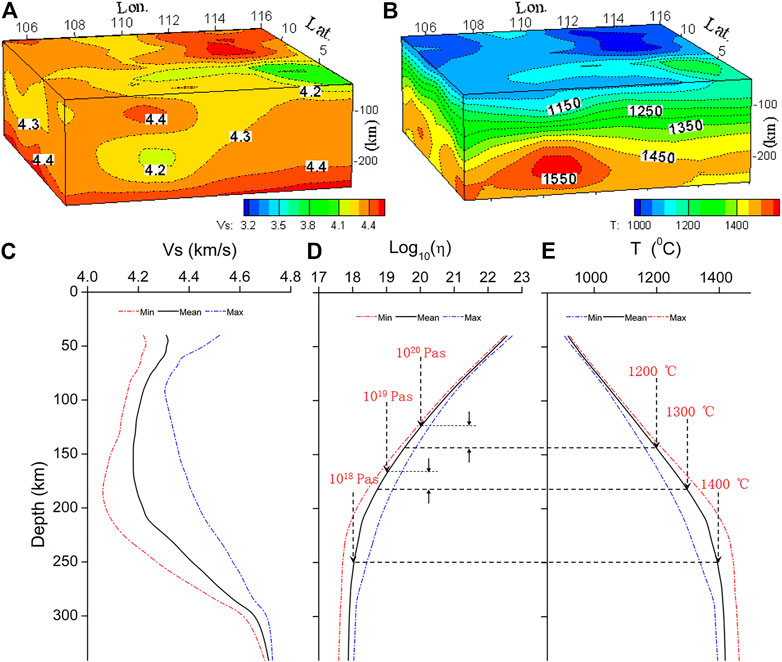
FIGURE 6. Diagram of the S-wave velocity characteristics and dynamic analysis of the mantle in the southwestern margin of SCS. (A) S-wave velocity 3D model (km/s). (B) Temperature chart (50–250 km) calculated by wave velocity model (°C). (C) Average S-wave velocity structure varying with depth. (D) Logarithm of the effective viscosity coefficient of the mantle with variations at depth. (E) Mantle temperature varying with depth.
Theoretically, S wave velocity is determined by shear modulus and density, and it is related to temperature, pressure, mineral composition and structure, fluid, and other parameters (Nolet and Zielhuis, 1994; Sobolev et al., 1996). Due to the lack of measured data on the lithologic structure of the upper mantle in the western margin of SCS, it is assumed that the proportion of lithologic components in the upper mantle is, respectively, as follows: olivine—68%, orthopyroxene—18%, clinopyroxene—11%, and garnet—3% (Goes et al., 2000; An and Shi, 2007). According to the lithologic components, the temperature distribution of the upper mantle in the strike–slip fault zone can be inverted from the Vs wave velocity by means of Eq. 2 (Figure 6B). According to the results in Figure 6B and Eq. 3, the viscosity distribution corresponding to temperature can be calculated.
The new-generation 3D shear wave velocity model proposed by Chen et al. (2021) is only available for up to 250-km depth. Considering that its deep wave structure is similar to that proposed by Mei and An (2010), we integrated the Vs data at a depth of 250–400 km from the model of Mei and An (2010) into the model of Chen et al. (2021). The model is expanded to marine shear wave model available for a deep dynamic analysis of the southwestern margin of the SCS. The average velocity, effective viscosity coefficient, and temperature curve of the upper mantle that varied with depth are calculated (Figure 6C−E). Figure 4C shows the variation in the Vs shear wave velocity with depth obtained by averaging statistics layer by layer. It can be seen that, at a depth range of 50–200 km, the shear wave velocity VS gradually decreases with depth, and the average velocity decreases from 4.36 to 4.17 km/s. In the depth from 200 to 300 km, the Vs value gradually increases, and the average velocity gradually rises from 4.17 to >4.6 km/s. Figures 6D,E show the variation of the logarithm of effective viscosity coefficient η of the mantle with depth and the variation of the mantle temperature T with depth obtained by averaging the mantle temperature and viscosity layer by layer. By comparing Figures 6D, E, it can be found that η is “mirroring” and symmetrical with T in the depth range of 50–300 km. Near the depth of 150 km, the average temperature of the mantle reaches 1,200°C, and the average effective viscosity coefficient is 1019–1020 Pa⋅s; at 180-km depth, the average temperature of the mantle is 1,300°C, and the average effective viscosity coefficient is at 1018–1019 Pa⋅s; at 250-km depth, the average temperature of the mantle is 1,400°C, and the average effective viscosity coefficient is slightly less than 1018 Pa⋅s. Below the depth of 180 km, the temperature and viscosity can meet the temperature and viscosity conditions required for partial melting or convective migration of the mantle material (Milne G A, et al., 2001; Mitrovica J X, et al., 2004).
The convective activity in the upper mantle asthenosphere is an important element in the creation of lithospheric tectonic dynamics, magmatic activity, and material circulation. The asthenosphere is closely related to the seismic low-velocity zone, and the asthenospheric mantle convection controlled by the viscosity structure may cause the geoid to have positive and negative anomalies. Therefore, the geoid anomaly is an essential constraint for calculating the convective viscosity structure of the mantle. By constraining the velocity–density–temperature conversion factor with the geoid (WGM 2012) R-squared, the viscosity change of the upper mantle can be calculated. Note that this viscosity rheology is different from the above-mentioned lithospheric thermal rheology. Viscosity is the key parameter for controlling the mantle convection. Under the condition that the viscosity structure of the mantle is determined, the stress conditions that drive the mantle convection can be set up to calculate the convective velocity field of the mantle asthenosphere. The stress that drives the mantle convection can originate from density differences. Temperature change may affect the density of convective material, and density change may lead to convective activity. The heat convection equation describing this density change includes the following: the kinematic equation of a viscous fluid, the continuity equation under the assumption of incompressibility, and the heat transfer equation including the convection term, i.e., Eq. 5.
Based on the temperature model and thermal viscosity structure obtained from the seismic Vs analysis, the gravimetric geoid anomaly model (WGM 2012) was used to calculate the convection of the mantle asthenosphere (Figure 7). The global geoid anomaly map (Figure 7A) shows that the southwestern margin of the SCS is located between the negative anomaly zone of the Indian Ocean geoid and the positive anomaly zone of the Pacific geoid. The geoid height anomaly in the study area is at −15.56–58.86 m (Figure 7B). Overall, it is a geoid anomaly cascade that is low in NW and high in SE. The geoid height in the northwest corner is negative, while the geoid height in the southeast corner is positive. Figures 7C,D show the convective velocity field at 200–400-km depth in the mantle asthenosphere in the southwestern margin of the SCS as calculated by Eq. 5 under the constraints of the geoid model and seismic shear wave model. By comparing the convective velocity field of the mantle at the depth of 200–400 km, it can be found that the flow direction of the mantle asthenosphere varies greatly from shallow to deep area. At 200-km depth, the material flows toward the nearly south–north direction in the eastern continent of Vietnam. The flow changes to the east–south direction in the middle part and changes to nearly east–west direction beneath Borneo Island. The flow velocity is at 4.85–10.63 cm/a, which gradually decreases from northwest to southeast. At 200-km depth, the overall flow direction changes to east–west direction. The flow velocity is at 1.58–3.09 cm/a. There are two velocity zones, i.e., northwest and southeast. The northwest is a low-velocity zone, while the southeast is a high-velocity zone. The flow velocity at 400-km depth is not only greatly smaller than that at 200-km depth but also the distributions of high- and low-velocity zones are completely opposite. Figure 7E shows the variation of convective velocity of asthenosphere with depth. It can be seen that the material flow velocity gradually increases from 150 km below, and at 200-km depth, the flow velocity reaches a maximum value, which can reach an average of 8.5 cm/a. At 200-km depth or below, the material flow velocity gradually decreases. At 300-km depth, the average flow velocity decreases to 6.7 cm/a. At 400-km depth, the average flow velocity decreases to 2.2 cm/a.
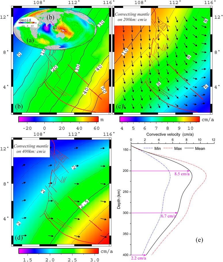
FIGURE 7. Analysis of convection in the upper mantle asthenosphere of the southwestern margin of South China Sea (SCS). (A) Global geoid anomaly (m). (B) Geoid anomaly (m) in the southwestern margin of SCS. (C) Convective velocity of the mantle at 200-km depth (cm/a). (D) Convective velocity of the mantle at 400-km depth (cm/a). (E) Variation of convective velocity of the asthenospheric mantle with depth (cm/a).
Discussion and Conclusion
New and Old Heat Flow Data
In the area where 30 sites of new heat flow data were present (Figure 1B and Figure 3), there are also 23 sites of previous heat flow data (Yao et al., 1994; Nissen et al., 1995). Figure 8 shows the comparison of overall 53 heat flow data.
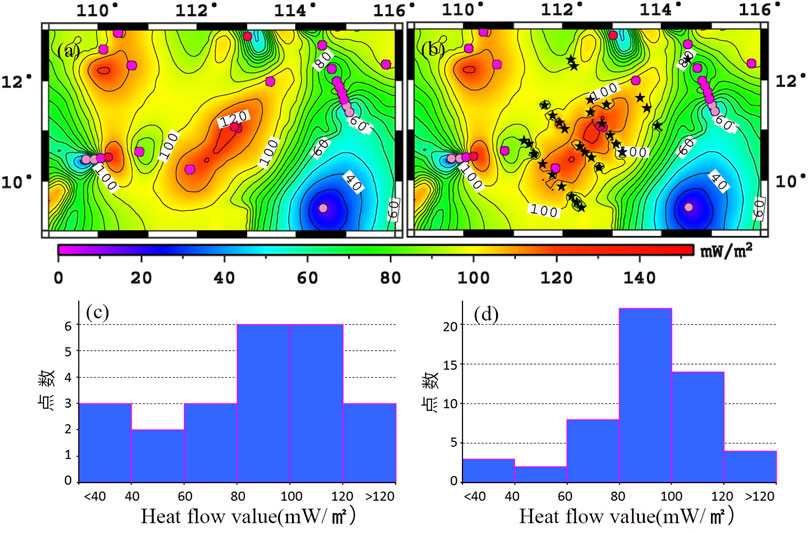
FIGURE 8. Comparison and analysis of new and old submarine heat flow data. (A) Submarine heat flow map with previous data. (B) Submarine heat flow map with the added new data. (C) Diagram of statistical distribution using the old data. (D) Diagram of statistical distribution using the added new data.
Figures 8A,C are diagrams of distribution and statistics of heat flow from 23 old data, while Figures 8B,D are diagrams of distribution and statistics of heat flow from the added 30 new data. The average heat flow value of 23 old data is 86.86 mW/m2, with a large difference between high and low heat flow values and a high dispersion (Figure 8C). After the inclusion of 30 new data, the average heat flow value in the study area is 91 mW/m2, and the distribution interval is relatively reasonable (Figure 8D). However, after a comparison between the results in Figures 8A,B, it seems that the addition of new data does not change the overall distribution pattern of submarine heat flow. Instead it only changes the detailed distribution of the heat flow in local areas. Therefore, in addition to making full use of the dynamic information obtained from the 30 new data, taking advantage of previous submarine heat flow data still lays an important foundation for geothermal analysis in the whole region.
Mantle Viscosity and Rheological Boundary Layer
The effective viscosity coefficient of the mantle depends on temperature, pressure, grain size, water content, etc. The higher the temperature, the lower the viscosity coefficient, and the higher the pressure, the higher the viscosity coefficient. In the uppermost mantle, the effective viscosity coefficient is mainly related to temperature, and the viscosity coefficient decreases with depth as temperature increases. However, in the deep mantle (below the asthenosphere and the lower mantle), due to the adiabatic (isothermal) compression effect, the pressure that increased with depth will make the viscosity coefficient increase with depth, which is greater than the effect that the temperature increase will have to make the viscosity coefficient decrease. Therefore, the viscosity tends to increase with depth, while the viscosity coefficient will not decrease gradually until the base of the mantle. Figure 9A shows the variation of the normalized mantle viscosity coefficient with depth calculated from different mineral physical constraint models (Steinberger and Arthur, 2006), from which it can be found that the viscosity of the mantle has a strong depth dependence, and the viscosity structure of the upper and lower mantles is very different.
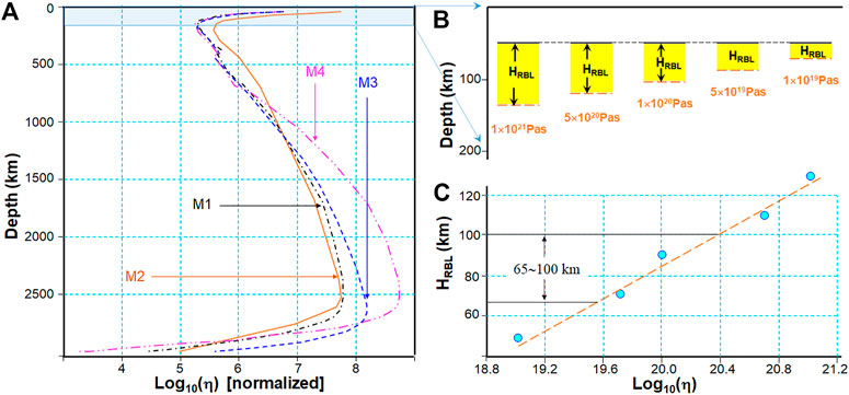
FIGURE 9. Analysis of mantle viscosity and rheological boundary. (A) Normalized mantle viscosity model (Steinberger and Arthur 2006). (B), (C) Changes of rheological boundary layer with mantle viscosity (He, 2014).
The viscosity coefficient of the upper mantle based on the post-glacial rebound and gravity equilibrium is 4–10 × 1020 Pa⋅s (Mitrovica and Forte, 2004). The GPS space geodetic study has obtained the asthenosphere viscosity coefficient of 5–10 × 1020 Pa⋅s (Milne et al., 2001), and the viscosity coefficient of the asthenosphere obtained from GRACE satellite gravity data and relative sea level data is 5.3 × 10²⁰ Pa⋅s (Paulson et al., 2010). The viscosity coefficient of the asthenosphere in the lower part of the oceanic lithosphere is about 7 × 10¹⁸ Pa⋅s (Doin et al., 1997), and the viscosity coefficient of the asthenosphere below the active tectonic region of the continental lithosphere is about 1018–1019 Pa⋅s (Dixon et al., 2004). The effective viscosity coefficient of the low-velocity layer in the upper mantle in the southwestern margin of the SCS is at 1018–1020 Pa⋅s (Figure 6D), which is consistent with the results of previous studies.
The effective viscosity coefficient of the mantle is not only the key parameter controlling the mantle convection but also the key factor controlling the thickness and the bottom boundary of the upper rheological boundary layer. According to the change characteristics of the geothermal gradient curve (Figure 2), the upper mantle can be divided into three layers: the upper is a pure conduction layer, the middle is a rheological boundary layer with a thickness of HRBL, in which heat conduction and heat convection coexist, and the geothermal gradient drops to below 4–5°C/km; the lower is a pure convection layer, in which the geothermal gradient is very small, and the adiabatic temperature gradient is 0.5°C/km. Due to the coexistence of conduction and convection, there is no obvious interface between the solid lithosphere and the fluid mantle in the RBL, and the bottom boundary is mainly affected by the effective viscosity coefficient of the mantle (He, 2014). The higher the effective viscosity coefficient of the mantle, the thicker the rheological boundary layer HRBL, and the lower the effective viscosity coefficient of mantle, the thinner the rheological boundary layer HRBL. Based on this, it is inferred that if the log10(η) of the asthenosphere in the southwestern margin of the SCS decreases from 20 to 18, the bottom of the rheological boundary layer (Figure 9B) or the thickness (Figure 9C) can be uplifted from 100 km or thinned to 65 km.
Conclusion
The southwestern margin of the SCS is located on the transition zone between the continental shelf and the slope. The strike–slip fault zone that runs through this zone has formed an important Cenozoic ocean–continent tectonic boundary. The strike–slip fault zone constrains the overall tectonic framework of the western margin of the South China Sea, and it is a key structural zone for understanding the geological evolution and continental margin dynamics of the SCS. The main study conclusions of this paper are as follows:
1. The newly acquired 30 submarine heat flow data have facilitated the study of geothermal field and thermal state in the western margin of the SCS. After the merging of new and old geothermal data, there is a series of submarine high-heat-flow areas along the strike–slip fault zone, of which the southern section of Zhongjiannan Basin, the southwestern margin of the Southwest Basin in the SCS, Wanan Basin, and Zengmu Basin are all at high-value areas with a heat flow of >90 mw/m2, whereas Nansha Island and Reef Area as well as Nansha Trough are at the low-value areas of submarine heat flow. The proportion of the crust and mantle components of the submarine heat flow in this area shows a clear NNE-trending strip-shaped distribution pattern. The southwest sea area along the axis of the Southwest Basin and the Zengmu Basin are of high-value areas of Qm/Qs >70%, in which the heat from the mantle is much higher than that of the crust, so it is a “hot mantle” strip, whereas Nansha Block has low mantle heat and is a “cold mantle” area with a low Qm/Qs value.
2. The Moho temperature calculated with the submarine heat flow data in this area is between 200 and 950°C. The Moho temperature in the Nansha sea area is the lowest, while the Moho temperature in the southern part of the Zengmu Basin is the highest, reaching >900°C. The Moho temperature in the Wanan Basin is also higher, which can reach over 800°C in some areas. The highest Moho temperature in the Zhongjiannan Basin is around 600°C. The strike–slip fault zone in the western margin of the SCS bends to the southeast into the Lupal Fault Zone and Tinja Fault Zone, beneath which the Moho temperature is obviously high, indicating that the deep geothermal activity caused by tectonic activity is intense. In the thermal–rheological structure of the lithosphere, there are two low-viscosity-coefficient regions at Moho depth on both the east and west sides of the strike–slip fault zone, with a viscosity coefficient at 1021–1022 Pa⋅s. Beneath the Nansha Block is a high-viscosity-coefficient region that is vertically extended, with a viscosity coefficient at 1024–1025 Pa⋅s. Beneath the Zengmu Basin is a “weak rheological zone” with a viscosity coefficient of less than 1020 Pa⋅s near the Moho, and partial melting magmatism may exist.
3. The new-generation high-resolution 3D shear wave velocity model for SCS can clearly reflect the tectonic characteristics at various depths. In the southwestern margin of SCS, if the Vs velocity structure is above the Moho, it mainly reflects the changes in ocean–continent tectonics; if the Vs velocity structure is beneath the Moho surface, it mainly shows the characteristics of the strike–slip fault structure in the western margin of the SCS. A low-velocity uplift from the mantle corresponding to the strike–slip structure appears to be beneath the study area. Below the depth of 100 km, the characteristics of the strike–slip structure are gradually weakening; below the depth of 200 km, the seismic shear wave velocity reflects the characteristics of material migration in the mantle asthenosphere and deep dynamic process. After entering the mantle, there is a low-velocity layer below the depth of 180 km. According to the conversion calculation of velocity–density–temperature constrained by a gravimetric geoid model, the average temperature of the mantle at 250-km depth can reach 1,400°C, and the average effective viscosity coefficient is close to 1018 Pa·s, which meets the temperature and viscosity conditions for partial melting or convective migration of mantle material.
4. The calculation results of the north and east shear stress components τN and τE in the rheological boundary layer show that the closer upward to the Moho surface, the greater the absolute value of τN and τE, and the closer the seismic shear low-velocity layer is, the smaller the absolute τN and τE. At 65-km depth, τN is at −5.78–6.32 × 10⁸ N/m2, and τE is at −11.09–8.66 × 10⁸ N/m2. At 100-km depth, both τN and τE are at −1–1 × 10⁸ N/m2. The thickness and the bottom depth of the rheological boundary layer are mainly controlled by the effective viscosity coefficient of the lower convective mantle layer.
5. The partial melting depth zone of the upper mantle material in the southwestern margin of the SCS roughly corresponds to the location of a low-velocity layer of the seismic shear wave beneath the lithosphere. Based on this, it can be inferred that the depth zone where the low-velocity layer and the partial melting of the mantle overlap is the convective layer where the material of the upper mantle migrates. The convective velocity of the mantle varies greatly from 200 to 400 km at depth. At 200-km depth, the average convective velocity is 8.5 cm/a, gradually decreasing from northwest to southeast; at 400-km depth, the average flow velocity is 2.2 cm/a. The flow velocity at 400-km depth is not only smaller than that at 200 km depth but also the distributions of high- and low-flow velocity areas are also opposite.
Data Availability Statement
The raw data supporting the conclusion of this article will be made available by the authors without undue reservation.
Author Contributions
All authors listed have made a substantial, direct, and intellectual contribution to the work and approved it for publication.
Funding
This study was supported by NSFC-Guangdong Joint Fund (grant no. U20A20100), Key Special Project for Introduced Talents Team of Southern Marine Science and Engineering Guangdong Laboratory (Guangzhou) (grant no. GML2019ZD0201), the National Natural Science Foundation of China (Grant No.42106079), National Natural Science Foundation Youth Fund (grant no. 42106079), Guangdong Natural Science Fund Research Team (grant no. 2107A030312002), Basic Marine survey project (Grant No. DD20221712, DD20221719) and National Marine and Land Mineral Resources Map Compilation and Update Project (grant no. DD20190368).
Conflict of Interest
The authors declare that the research was conducted in the absence of any commercial or financial relationships that could be construed as a potential conflict of interest.
The reviewer MZ declared a shared affiliation, with no collaboration, with one of the authors, HL, to the handling editor at the time of the review.
Publisher’s Note
All claims expressed in this article are solely those of the authors and do not necessarily represent those of their affiliated organizations or those of the publisher, the editors, and the reviewers. Any product that may be evaluated in this article or claim that may be made by its manufacturer is not guaranteed or endorsed by the publisher.
Acknowledgments
We are grateful to Zhiwei Li and Meijian An for their extremely helpful discussions and suggestions which have helped to significantly improve the manuscript. Two reviewers and scientific editors are thanked for their very careful reviews and constructive suggestions, which greatly enhanced the scientific and technical level of the paper.
References
An, H., Li, S., Suo, Y., Liu, X., Dai, L., Shan, Y., et al. (2012). Basin-controlling Faults and Formation Mechanism of the Cenozoic Basin Groups in the Western Margin of South China Sea. Mar. Geology. Quat. Geology. 31 (6), 95–111.
An, M., and Shi, Y. (2007). Three-dimensional Temperature Field of the Crust and Upper Mantle in Chinese Mainland. Sci. China (D) 37 (6), 736
Bowin, C. (1983). Depth of Principal Mass Anomalies Contributing to the Earth’s Geoid Undulations and Gravity Anomlies. Mar. Geodesy 7, 61–101. doi:10.1080/15210608309379476
Chen, H., Li, Z., and Luo, Z. (2021). Crust and Upper Mantle Structure of the South China Sea and Adjacent Areas from the Joint Inversion of Ambient Noise and Earthquake Surface Wave Dispersions. Geochem. Geophys. Geosystems 22, e2020GC009356. doi:10.1029/2020gc009356
Ding, W., and Li, J. (2016). Conjugate Margin Pattern of the Southwest sub-basin, south china Sea: Insights from Deformation Structures in the Continent-Ocean Transition Zone. Geol. J. 51, 524
Dixon, J. E., Dixon, T. H., and Bell, D. R. (2004). Lateral Variation in Upper Mantle Viscosity: Role of Water. Earth Planet. Sci. Lett. 222 (2), 451–467. doi:10.1016/j.epsl.2004.03.022
Doin, M. P., Fleitout, L., and Christensen, U. (1997). Mantle Convection and Stability of Depleted and Undepleted Continental Lithosphere. J. Geophys. Res. Solid Earth 102 (B2), 2771–2787. doi:10.1029/96jb03271
Dong, M., Wu, S., Zhang, J., Xing, X., Gao, J., and Song, T. (2020). Lithospheric Structure of the Southwest South China Sea: Implications for Rifting and Extension. Int. Geology. Rev. 62 (7-8), 924–937. doi:10.1080/00206814.2018.1539926
Dong, M., Zhang, J., Xu, X., and Wu, S.-G. (2018). The Differences between the Measured Heat Flow and BSR Heat Flow in the Shenhu Gas Hydrate Drilling Area, Northern South China Sea. Energy Exploration & Exploitation 37, 756–769. doi:10.1177/0144598718793907
Fu, R., Huang, J., and Liu, W. (1994). Correlation Equation between Regional Gravity Isostatic Anomalies and Small Scale Convection in the Upper Mantle. Chin. J. Geophys. 37, 638
Fukao, Y., Obayashi, M., Inoue, H., and Nenbai, M. (1992). Subducting Slabs Stagnant in the Mantle Transition Zone. J. Geophys. Res. 97, 4809–4822. doi:10.1029/91JB02749
Fyhn, M., Boldreel, L. O., and Nielsen, L. H. (2009). Geological Development of the Central and South Vietnamese Margin:Implications for the Establishment of the South China Sea, Indochinese Escape Tectonics and Cenozoic Volcanism. Tectonophysics 478 (3), 184–214. doi:10.1016/j.tecto.2009.08.002
Gao, H. (2011). A Tentative Discussion on Strike-Slipping Character and Formation Mechanism of Western-Edge Fault Belt in South China Sea. Geology. China 10 (03), 537
Goes, S., Govers, R., and Vacher, P. (2000). Shallow Mantle Temperatures under Europe from P and S Wave Tomography. J. Geophys. Res. 105 (B5), 11153–11169. doi:10.1029/1999jb900300
He, L. (2014). The Rheological Boundary Layer and its Implications for the Difference between the Thermal and Seismic Lithospheric Bases of the North China Craton. Chin. J. Geophys. 57 (1), 53
Huang, J., and Zhao, D. (2006). High-resolution Mantle Tomography of China and Surrounding Regions. J. Geophys. Res. 111, B9. doi:10.1029/2005JB004066
Li, J., Ding, W., Wu, Z., Zhang, J., and Dong, C. (2012). The Propagation of Seafloor Spreading in the Southwestern Subbasin, South China Sea. Chin. Sci. Bull. 57 (24), 3182–3191. doi:10.1007/s11434-012-5329-2
Li, Y., Luo, X., and Xing, X. (2010). Seafloor In-Situ Heat Flow Measurements in the Deep-Water Area of the Northern Slop, South China Sea. Chin. J. Geophys. 53 (9), 2161–2170. doi:10.1002/cjg2.1547
Lin, C., Tang, Y., and Tan, Y. (2009). Geodynamic Mechanism of Dextral Strike-Slip of Western-Edge Faults of the South China Sea. Acta Oceanologica Sinica (Chinese Version) 29 (01), 159
Lin, M., and Zhang, J. (2014). Thermal Simulation on Magma Activity Mechanism of Residual Ridge in the Southwest Basin of the South China Sea. Sci. China (D) 44 (6), 239
Liu, B., Xia, B., Li, X., Zhang, M., Niu, B., Zhong, L., et al. (2006). Southeastern Extension of the Red River Fault Zone (RRFZ) and its Tectonic Evolution Significance. Sci. China (D) 36 (10), 914
Liu, H. (1999). On an Extension-contraction-type Dextral Strike-Slip Duplex System in Western Nansha Waters of South China Sea and its Dynamic Process. Mar. Geology. Quat. Geology. 19 (3), 11
Liu, H., Yao, Y., Shen, B., Cai, Z., Zhang, Z., Xu, H., et al. (2015). On Linkage of the Western Boundary Faults of the South China Sea. Earth Scienc 40 (4), 615–632
Lu, L., Stephenson, R., and Clift, P. D. (2016). The canada basin Compared to the Southwest south china Sea: Two Marginal Ocean Basins with Hyper-Extended Continent-Ocean Transitions. Tectonophysics 691, 171
Mei, F., and An, M. (2010). Lithospheric Structure of the Chinese Mainland Determined from Joint Inversion of Regional and Teleseismic Rayleigh-Wave Group Velocities. J. Geophys. Res. 115, B06317. doi:10.1029/2008JB005787
Milne, G. A., Davis, J. L., and Mitrovica, J. X. (2001). Space-geodetic Constraints on Glacial Isostatic Adjustment in Fennoscandia. Science 291 (5512), 2381–2385. doi:10.1126/science.1057022
Mitrovica, J. X., and Forte, A. M. (2004). A New Inference of Mantle Viscosity Based upon Joint Inversion of Convection and Glacial Isostatic Adjustment Data. Earth Planet. Sci. Lett. 225 (1), 177–189. doi:10.1016/j.epsl.2004.06.005
Nissen, S. S., Hayes, D. E., and Bochu, Y. (1995). Gravity, Heat Flow, and Seismic Constraints on the Process of Crustal Extension: Northern Margin of the South China Sea. J. Geophys. Research:Solid Earth 100 (B11), 22447–22483. doi:10.1029/95jb01868
Nolet, G., and Zielhuis, A. (1994). Low S Velocities under the Tornquist-Teisseyre Zone: Evidence for Water Injection into the Transition Zone by Subduction. J. Geophys. Res. 99, 15813–15820. doi:10.1029/94jb00083
Paulson, A., Zhong, S., and Wahr, J. (2010). Inference of Mantle Viscosity from GRACE and Relative Sea Level Data. Geophys. J. Int. 171 (2), 497
Qian, Y. (1992). Survey and the Results of Geothermal Flow in the Northern Part of South China Sea. Mar. Geology. Quat. Geology. 2 (4), 102
Ren, J., and Li, S. (2000). Expansion Process and Dynamic Background of the Western Pacific Marginal Basin. Earth Sci. Front. 7 (3), 203
Runcorn, S. K. (1967). Flow in the Mantle Inferred from Low Degree Harmonics of the Geopotential. J. Geophys. Res. 72, 375
Runcorn, S. K. (1964). Satellite Gravity Measurements and a Laminar Viscous Flow Model of the Earth’s Mantle. J. Geophys. Res. 69, 4389–4394. doi:10.1029/jz069i020p04389
Shi, X., Qiu, X., and Xia, K. (2003). Characteristics of Surface Heat Flow in the South China Sea. J. Asian Earth Sci. 22 (3), 265–277. doi:10.1016/s1367-9120(03)00059-2
Sobolev, S. V., Zeyen, H., and Stoll, G. (1996). Upper Mantle Temperatures from Teleseismic Tomography of French Massif Central Including Effects of Composition, Mineral Reactions, Anharmonicity, Anelasticity and Partial Melt. Earth Planet. Sci. Lett. 139, 147–163. doi:10.1016/0012-821x(95)00238-8
Steinberger, B., and Arthur, R. C. (2006). Models of Large-Scale Viscous Flow in the Earth’s Mantle with Constraints from Mineral Physics and Surface Observations. Geophys. J. Int. 167 (4), 1461–1481. doi:10.1111/j.1365-246x.2006.03131.x
Sun, Z., Zhong, Zg., Zhou, D., Xia, B., Qiu, X., Zeng, Z., et al. (2006). Study on Developmental Mechanism of South China Sea: Evidence from Similar Simulations. Sci. China (D) 36 (09), 797
Tapponnier, P., Peltzer, G., and Armijo, R. (1986). On the Mechanics of the Collision between India and Asia. Geol. Soc. Lond. Spec. Publications 19 (1), 113–157. doi:10.1144/gsl.sp.1986.019.01.07
Wang, P., Huang, C., Lin, J., Zhimin, J., Sun, Z., and Zhao, M. (2019). The south china Sea Is Not a mini-atlantic: Plate-Edge Rifting vs Intra-plate Rifting. Natl. Sci. Rev. 6 (05), 54–65. doi:10.1093/nsr/nwz135
Wu, J., and Liu, Y. (1992). A Study on the Relation between Satellite Gravity Anomalies, Mantle Convection Stress and Modern Plates Movement. Acta Geophysica Sinica 35 (5), 604
Xing, X., Lu, J., and Luo, X. (2005). The Marine Heat Flow Survey and the Result Discussion in the Northern Part of South China Sea. Prog. Geophys. 20 (2), 562
Xing, X., Yao, Y., and Deng, P. (2018). The Characteristics and Analysis of Heat Flow in the Southwest Sub-basin of South China Sea. Chin. J. Geophys. 61 (7), 2915
Xu, Z., Wang, Q., Li, Z., Li, H., Cai, Z., Liang, F., et al. (2016). Indo-Asian Collision: Tectonic Transition from Compression to Strike Slip. Acta Geologica Sinica 90 (01), 1
Yao, B., Wan, L., and Wu, N. (2004). Cenozoic Plate Tectonic Activities in the Great South China Sea Area. Geology. China 31 (2), 113–122.
Yao, B., Zeng, W., and Hayes, D. E. (1994). The Geological Memoir of South China Sea Surveyed Jointly by China and USA. Wuhan: China University of Geosciences Press, 140
Yao, Y., Yang, C., Li, X., Ren, J., Jiang, T., Dianjun, X., et al. (2013). The Seismic Reflection Characteristics and Tectonic Significance of the Tectonic Revolutionary Surface of Mid-Miocene (T3 seismic interface) in the Southern South China Sea8 Zhang Jian, Dong Miao, Wu Shiguo, et al. 2017. Lithosphere Thermal-rheological Structure and Geodynamic Evolution Model of the Nansha Trough Basin, South China Sea. Chin. J. GeophysicsEarth Sci. Front. 5624 (43), 127427
Zhan, W., Liu, Y., and Zhong, Ji. (1995). The Preliminary Analysis of Neotectonic Movement and Dynamic Evolution in the Southern DIWA Region of South China Sea. Geotectonica Et Metallogenia 19 (2), 95
Zhang, J., Song, H., and Li, J. (2005). Thermal Modeling of the Tectonic Evolution of the Southwest Sub-basin in the South China Sea. Chin. J. Geophys. 48 (6), 1357
Zhang, J., and Wang, Jg. (2000). The Deep Thermal Characteristic of Continental Margin of the Northern South China Sea. Chin. Sci. Bull. 145 (10), 1095–1100. doi:10.1007/bf02898994
Keywords: south of the western margin of the South China Sea, submarine heat flow, three-dimensional Vs model, crust–mantle thermal–rheological structure, rheological boundary of lithospheric mantle, asthenosphere of upper mantle
Citation: Yao Y, Zhang J, Dong M, Zhu R, Xu Z, Yang X and Liu H (2022) Geodynamic Characteristics in the Southwest Margin of South China Sea. Front. Earth Sci. 10:832744. doi: 10.3389/feart.2022.832744
Received: 13 December 2021; Accepted: 07 February 2022;
Published: 26 April 2022.
Edited by:
Xunhua Zhang, Qingdao Institute of Marine Geology (QIMG), ChinaReviewed by:
Jiangxin Chen, Qingdao Institute of Marine Geology (QIMG), ChinaMinghui Zhao, South China Sea Institute of Oceanology (CAS), China
Xingwei Guo, Qingdao Institute of Marine Geology (QIMG), China
Copyright © 2022 Yao, Zhang, Dong, Zhu, Xu, Yang and Liu. This is an open-access article distributed under the terms of the Creative Commons Attribution License (CC BY). The use, distribution or reproduction in other forums is permitted, provided the original author(s) and the copyright owner(s) are credited and that the original publication in this journal is cited, in accordance with accepted academic practice. No use, distribution or reproduction is permitted which does not comply with these terms.
*Correspondence: Jian Zhang, emhhbmdqaWFuQHVjYXMuYWMuY24=