Relationship Between Asperities and Velocity Pulse Generation Mechanism

Near-fault ground motion records often capture instances of pulse-like behavior, where a burst of energy is expressed as large wave amplitude that occur over short time. The pulse-like ground motion can cause serious damage to long-period structures. Using numerical simulations of near-fault ground motions, we analyze the mechanisms involved in the generation of velocity pulses in the 1994 Northridge Earthquake and the 1979 Imperial Valley Earthquake. The degree to which the asperities affect the pulse generation process is investigated by identifying individual velocity pulses from the superposition process of sub-fault ground motions. Pulse indicators E_p and PGV_p represent pulse characteristics in the ground motions at the stations located near the epicenter (near-epicenter stations) and the stations located along the forward rupture propagation direction of the asperity (rupture-direction stations), respectively. To observe the effects of the asperities and the spatial relationship between the pulse-like ground motion stations and the asperities, we determine the contribution of the sub-fault motions to the pulse amplitude. Furthermore, we analyze the pulse indicators and the frequency components using simulated ground motions from two different slip distributions. The near-epicenter station ground motions, produced by homogeneous slip distribution, exhibit higher pulse amplitude and more concentrated low-frequency energy than those generated by the inhomogeneous slip distribution. The rupture-direction station ground motions, produced by inhomogeneous slip distribution, present higher pulse amplitude and more concentrated low-frequency energy than those generated by the homogeneous slip distribution. Our analysis reveals that during the fault rupture process, the pulse energy and the pulse amplitude are influenced by both the slip distribution on the fault plane and the spatial relationship between the seismic station and the asperity.

Introduction

Near-fault ground motions, which are distinctly different from far-field ground motions, are influenced by propagation media, site conditions, and the nature of seismic source. Velocity pulse is one of the main features in near-fault ground motions, which may cause serious damage to long-period structures. This feature has received significant attention since Heaton et al. (1995) first revealed that pulse-like ground motions from the 1994 Northridge Earthquake imparted significant damage to base-isolated frame buildings. In the last decade, researchers have begun using certain indicators to identify and classify ground motions as pulse-like or non-pulse-like. Many techniques were developed to extract velocity pulses, including mathematical models (e.g., sinusoidal velocity model, acceleration model, multi-parameter attenuate velocity pulse model) (Mavroeidis and Papageorgiou, 2003; Zhai et al., 2013; Chang et al., 2020), time-frequency analysis (Baker, 2007; Shahi and Baker, 2011; Mimoglou et al., 2014; Shahi and Baker, 2014; Whitney, 2019; Sharbati et al., 2020; Tang et al., 2021), and empirical mode decomposition (EMD) (Huang et al., 1998; Xu and Agrawal, 2010; Chen and Wang, 2020). Despite these investigations, the mechanisms and processes that ultimately result in velocity pulses are not well known. Generally, pulse-like ground motions are mainly caused by the directivity effect, which appear when the fault rupture propagates towards a seismic station and the rupture velocity is close to the shear wave velocity of the medium. In this scenario, the seismic intensities are higher than those propagating in the opposite direction. Furthermore, the velocity pulse is also produced by other factors such as the permanent displacement caused by the fling step effect and soil conditions. Liu (2005), while exploring the relationship between velocity pulses and seismic source parameters, proposed that the pulse period and the pulse amplitude depended on the depth of the fault, the rupture starting point, and the asperity locations. Mena and Mai (2011) found that directivity pulse was strongly related to the slip distribution on the fault plane and the location and size of the asperities. While Jiang and Bai (2016) analyzed the energy released by these pulse-like ground motions and found that this energy heavily influenced the velocity pulse period, Fayjaloun et al. (2017) demonstrated that the geometry of the fault and the rupture velocity were the main factors affecting the pulse period. With respect to the velocity pulse generation mechanisms, Poiata et al. (2017) found that for dip-slip faults, the directivity effect played a leading role at footwall stations. The focusing effect was found primarily responsible for the generation of the velocity pulses at hanging wall stations (Kagawa, 2009). Scala et al. (2018) simulated the ground motion in the 2009 L'Aquila Earthquake and found that the appearance and duration of the velocity pulses were dependent on the rise time of the source, the average rise time, the station location, the rupture velocity, and the fault depth. Using the three-dimensional finite difference method (Luo, 2019; Luo et al., 2020) and the F-K method (Lin et al., 2019) to simulate the pulse-like ground motions from the 1999 Chi-Chi Earthquake (Taiwan, China), and the 2018 Hualian Earthquake (Taiwan, China), previous studies indicated that the rise time of the asperity and the fault depth informed the velocity pulse shape, period, and amplitude. Lin et al. (2019) further proposed that site effect and the presence of sub-fault promote the generation of velocity pulses. Using the spectral element method, Tsuda (2020) simulated the ground motions in the 2016 Kumamoto Earthquake and found that the seismic source parameters played a significant role in the generation of the velocity pulses. By modeling the near-fault ground motions in the 1994 Northridge Earthquake and the 1979 Imperial Valley Earthquake using the F-K method, Cao (2020) discovered that different mechanisms were responsible for the generation of the forward-directivity pulses and the other non-directivity pulses. The directivity pulses were caused by large-amplitude waveforms in near-fault region or by the superposition of sub-fault ground motions in the forward rupture propagation direction, while the other non-directivity pulses were mainly attribute to the reflection of S waves produced by seismic source radiation.

In this study, we analyzed the influence of asperities on the velocity pulses by comparing the observed and simulated ground motions for both the 1994 Northridge Earthquake and the 1979 Imperial Valley Earthquake. Widely used methods, such as time-frequency analyses and empirical mode decomposition (EMD), may reduce calculation efficiency and suppress signal amplitude. Therefore, we categorized and characterized the pulse behavior using mathematical model to fit the shape of the observed velocity pulses. In the simulated waveforms, each time series is produced by the rupture of sub-faults, and the final ground motion waveform is the superposition of these individual ground motions with a certain time lag. We observed the pulse indicators during the superposition process and quantify the contribution of each sub-fault to the final pulse amplitude. We then compared the pulse indicators and the frequency components of the simulated near-fault ground motions produced by two different slip distributions. Lastly, we preliminarily confirmed that the relationship between site location and asperity exerts a significant influence on the pulse generation process.

Data and Identification Method

Observed Ground Motions and Identification Method

In this study, we examined ground motions from a dip-slip event (the 1994 Northridge Earthquake) and a strike-slip event (the 1979 Imperial Valley Earthquake) by collecting the EW and NS components of 384 acceleration records from the Pacific Earthquake Engineering Research Center (http://ngawest2.berkeley.edu). To identify the velocity pulses in these time series, we use the peak point method (PPM) (Zhai et al., 2013). PPM is an energy-based pulse identification and extraction method that uses a simplified mathematical model to fit velocity pulses. The pulse model proposed by Dickinson and Gavin (2011) is expressed as:

${\nu }_p\left(t;V_p,T_p,N_c,T_{pk},\phi \right)=V_p\mathit{exp}\left[-\frac{{\pi }^2}{4}{\left(\frac{t-T_{pk}}{N_c{T}_p}\right)}^2\right]\times \mathit{cos}\left(2\pi \frac{t-T_{pk}}{T_p}-\phi \right)(1)$

where V_p is the peak amplitude (cm/s), T_p is the period (s), N_c is the number of fitted pulses, φ is the phase parameter, and T_pk is the peak moment (s). The least-squares method is used to fit the pulse model to the original signal. To simplify the model, we set N_c = 1 and φ = 0. T_p is defined as the time interval between adjacent peak ground velocity (PGV) peaks or troughs. The pulse period T_p, the pulse amplitude V_p and the pulse peak moment T_pk are calculated by finding the pulse model that best fits the pulses in the observed records. Figure 1 shows an example of a velocity pulse extracted using PPM. Eqs. 2, 3 are used to calculate the relative cumulative energy of the velocity time series:

$E\left(\tau \right)=\frac{{{\displaystyle \int }}_0^t{\upsilon }^2\left(\tau \right)d\tau }{{{\displaystyle \int }}_0^{\infty }{\upsilon }^2\left(\tau \right)d\tau }(2)$

$E_p={\displaystyle \underset{t_s}{\overset{t_e}{\int }}dE\left(t\right)}=E\left(t_e\right)-E\left(t_s\right)=\frac{{{\displaystyle \int }}_{t_s}^{t_e}{\upsilon }^2\left(\tau \right)d\tau }{{{\displaystyle \int }}_0^{\infty }{\upsilon }^2\left(\tau \right)d\tau }(3)$

where v(τ) is the velocity time series, E(t) is the cumulative energy of the velocity time series, E_p is the relative energy of the identified pulses, and t_s and t_e represent the starting point and ending point of the pulse, respectively. The threshold of the energy index E_p is set to 0.3 (Zhai et al., 2013). We also apply a criterion of PGV >30 cm/s to exclude low-amplitude ground motions from our analysis. We eliminate the effects of the seismometer orientation by rotating the acceleration histories from original EW and NS orientations to FP (Fault Parallel) and FN (Fault Normal) orientations. The two earthquakes yield a total of 27 records with FN orientations containing pulse-like ground motions (red triangles in Figure 2).

FIGURE 1

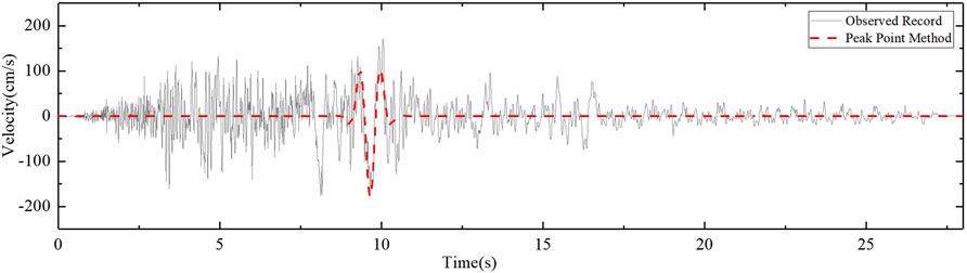
FIGURE 1. An example of pulse-like ground motion identified by PPM. The red dotted line represents the extracted pulse from the Northridge station in the Jensen Filter Plant Administrative Building.

FIGURE 2

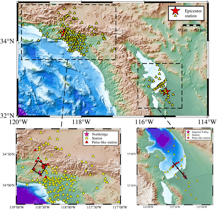
FIGURE 2. Seismic stations and surficial fault projections of the Northridge Earthquake and the Imperial Valley Earthquake.

Simulating Ground Motions With the F-K Method

To address the role of asperity in the pulse generation process, we utilize the F-K method, which is a semi-analytical frequency-wavenumber Green’s function method (Zhu and Rivera, 2002; Hartzell et al., 2005; Hartzell et al., 2011; Cao et al., 2019). The F-K method relies on wave theory to solve the Green’s function in the frequency-wavenumber domain and, when combined with a finite-fault source model, can be used to simulate the bedrock ground motions that occur during seismic events. We simulate acceleration time series from the 1994 Northridge Earthquake (83 time series) and the 1979 Imperial Valley Earthquake (31 time series) using the F-K method. The 1D velocity models in the 1994 Northridge region and the 1979 Imperial Valley region are from Graves and Pitarka (2010) and listed in Table 1. The source parameters, such as the fault size, strike angle, dip angle, and slip distribution, are sourced from the inversion results of Hartzell and Heaton (1983) and Wald et al. (1996) (Table 2).

TABLE 1

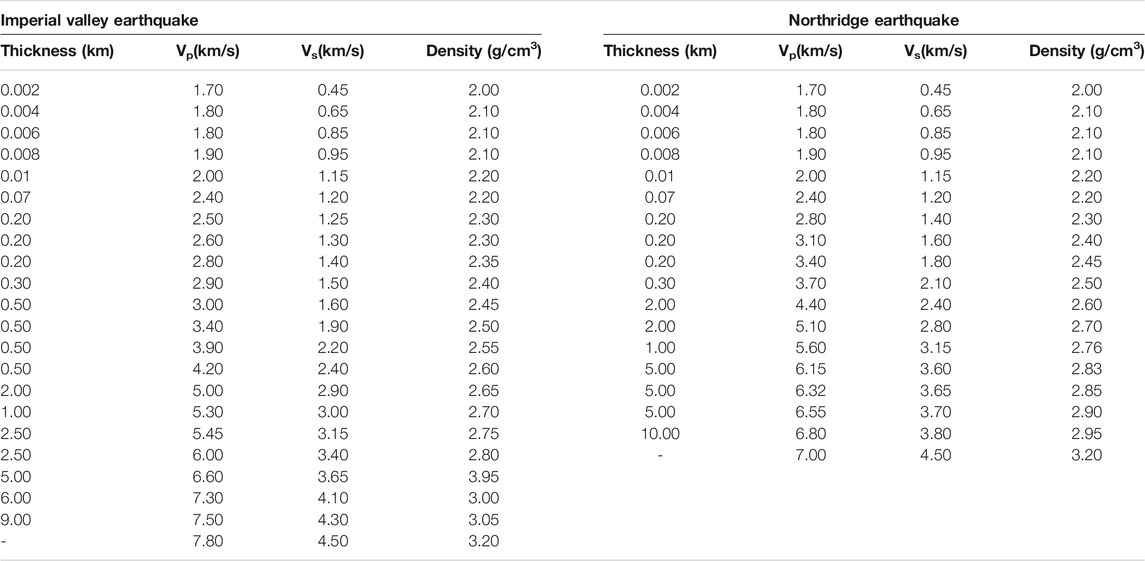
TABLE 1. Imperial Valley and Northridge region 1-D velocity profiles

TABLE 2

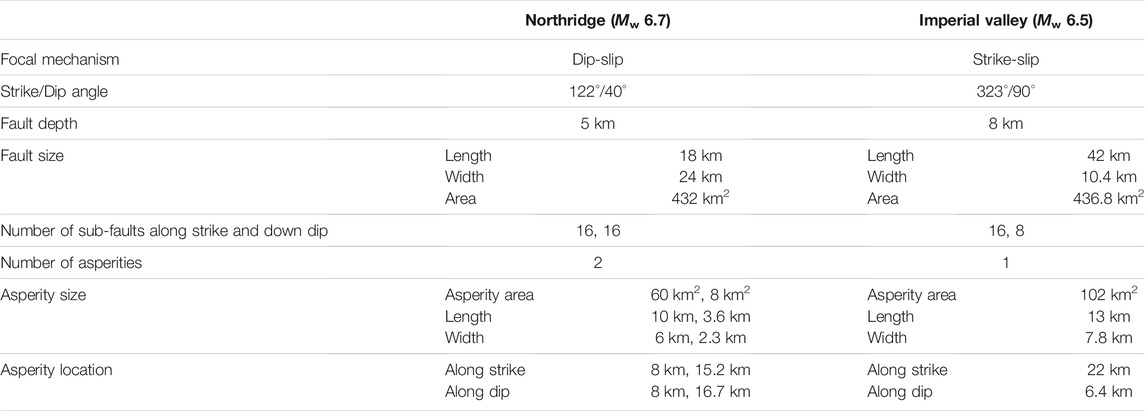
TABLE 2. Source parameters used in the F-K method ground motion simulations.

The pseudo spectral accelerations (PSA) of the simulated FN components are compared to the records from the 1994 Northridge Earthquake and 1979 the Imperial Valley Earthquake (Figure 3). Overall, the PSAs of the simulated ground motions are consistent with those of the observed PSAs throughout the entire period range.

FIGURE 3

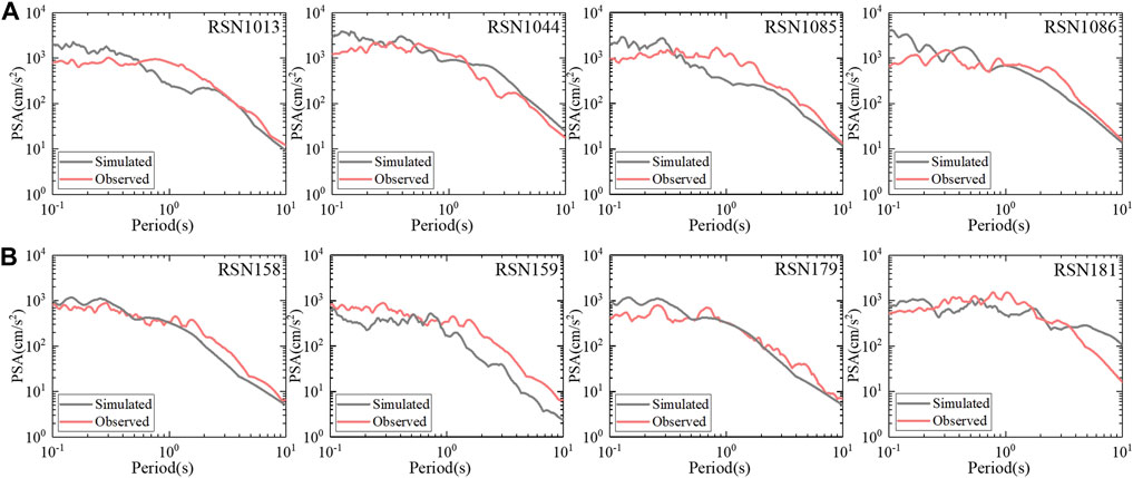
FIGURE 3. The simulated and observed response spectra produced by bedrock ground motion from (A) the Northridge Earthquake and (B) the Imperial Valley Earthquake.

For stations with complicated shear-wave velocity structure, we account for possible site effect such as sediment layer amplification. By inputting the upward wave of the simulated ground motions at bedrock (assuming a shear-wave velocity of 750 m/s), we use the Quarter-Wavelength method (QWL) proposed by Joyner et al. (1981) to model the frequency-dependent site effect. For example, the simulated, QWL, and observed spectral responses at four stations during the 1979 Imperial Valley Earthquake are shown in Figure 4. The shear-wave velocities of the soil layers at these stations are based on the values reported in Fumal et al. (1982) and Porcella (1984).

FIGURE 4

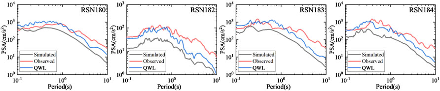
FIGURE 4. The simulated, observed, and QWL response spectra produced by ground motion at the bedrock and at the surface of four stations that recorded seismic data from the Imperial Valley Earthquake.

As shown in Figure 4, the response spectra of the surface ground motions are similar to those of the observed records at entire period. Of our 114 simulated ground motions, 27 motions contain pulse-like waveforms; however, several of the corresponding observed records are identified as non-pulse-like ground motions. We only select records where both the observed and simulated motions are identified as pulse-like motions for further analysis. The station information, pulse amplitude PGV_p, pulse period T_p and relative cumulative energy E_p for these selected records are listed in Table 3.

TABLE 3

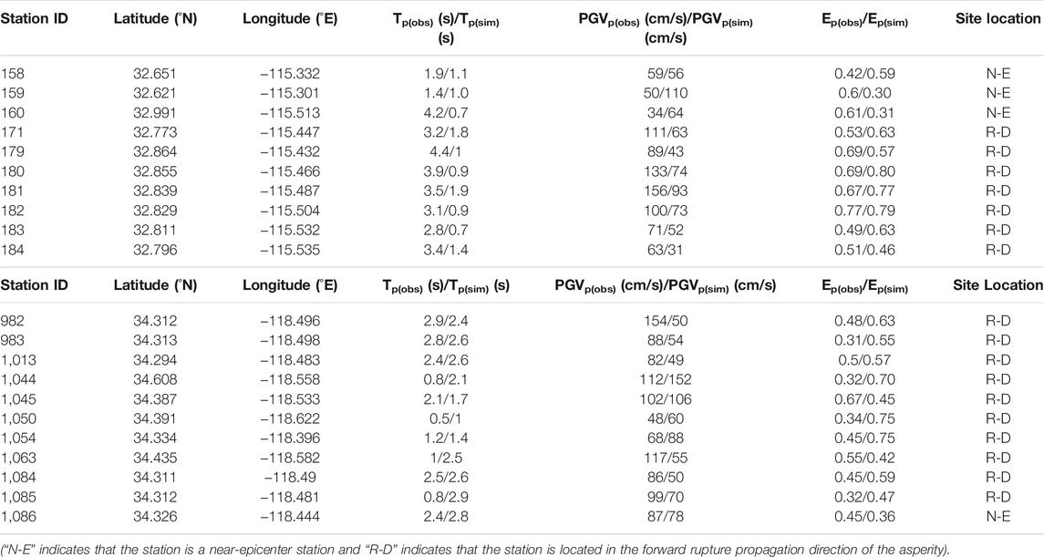
TABLE 3. Station information and pulse indicator values.

In the 1979 Imperial Valley Earthquake, the directivity effect causes the velocity pulses mostly appear in the FN component. However, in the 1994 Northridge Earthquake, most pulse-like ground motions occur at the hanging wall stations (Figure 2 and Table 3).

In Pulse Indicators in the Superposition of Sub-Fault Motions and Pulse Indicator Results, we use the PPM model to identify changes in the pulse indicators of the simulated pulse-like ground motions (listed in Table 3). Specifically, in the finite-fault source model, the fault plane is divided into N_L and N_W sub-faults in the along-strike and along-dip directions, respectively. From the rupture starting point, the sub-fault ground motions are superimposed sequentially in the time domain with an appropriate time delay, resulting in the final time series:

$a\left(t\right)={\displaystyle \sum _{i=1}^{N_L}{\displaystyle \sum _{j=1}^{N_w}{a}_{ij}}}\left(t-\left(\mathrm{\Delta }{t}_{ij}^{\prime }+\mathrm{\Delta }{t}_{ij}^{\prime \prime }\right)\right)(4)$

where a(t) represents the ground motion at a station and a_ij(t) is the ground motion produced by the rupture of sub-fault ij. The total time delay is the sum of Δt^′_ij and Δt^′_ij, which represent the rupture time of sub-fault ij and the propagation time from the starting point to sub-fault ij, respectively. At the relevant stations, we identify velocity pulses in each individual ground motion a_ij(t) to understand the influence exerted by the asperities by observing the time and position of the velocity pulses.

The Windowed Fourier Transform (WFT) of time-frequency analysis is conducted to express how the slip distribution affects the frequency components of the simulated ground motions in Pulse Indicator Results. The WFT applies an overlapping rectangular window of a certain time duration to each part of the time series and then calculates the Fourier transform of each windowed section in order to obtain the corresponding frequency spectrum. The relationship between the short-time Fourier window width (T_w) and the moment magnitude (M_w), investigated in the research of Mena and Mai (2011), is expressed as:

$T_w=-16.1+3.08M_w(5)$

For our analysis, the window width of the 1994 Northridge Earthquake and 1979 Imperial Valley Earthquake is 4 s, with the sampling rate of 50 Hz. The PPM model for identification velocity pulse and the Windowed Fourier Transform for time-frequency analysis can investigate the effect of spatial relations between the stations and asperities on the velocity pulse generation.

Effect of the Superposition of Sub-Fault Motions on the Generation of the Velocity Pulse

Pulse Indicators in the Superposition of Sub-Fault Motions

An asperity is the area on a fault where the rupture is temporarily stuck and the slip value is significantly higher than the values on other parts of the fault. The consensus is that fault asperity exists when the resulting slip is about 1.5–2 times larger than the average slip on that fault plane. Previous investigations have focused on how the sizes and locations of the asperities affect the ground motions in the near-fault region. For example, Somerville et al. (1997); Somerville et al. (1999); Somerville, (2003) applied deterministic parameters to describe the properties of the slip models for fifteen crustal earthquakes by using the asperities and the wavenumber spectra to quantify the slip heterogeneity. They analyzed the relationship between slip model and seismic moment, demonstrated that slip distribution greatly affected near-fault ground motions, and stated that the energy released by asperities represented a significant contribution to the total energy and seismic moment of these crustal earthquakes. Furthermore, the asperity dimensions somewhat inform the distribution of the near-fault ground motions (Wang, 2004). Existing research on this topic mostly focused on the influence of rupture velocity, rupture mode, rise time, and the number and position of asperities on pulse-like ground motions. Miyake et al. (2001); Miyake et al. (2003) demonstrated that the near-fault ground motions in the 0.2–20 Hz frequency range were related to the area of the asperities. Cao (2020) proposed that the pulse amplitude was largely dictated by the asperity size and location, that short-period ground motions were affected by the seismic source time function, that long-period ground motions depended on the spatial slip distribution, and that site effect, wave propagation, and the superposition process may also result in pulse-like ground motions.

This section discusses the effect of the asperities on the velocity pulses that arise during the superposition process of sub-faults in the fault plane. The PPM model is applied to identify changes in the pulse indicators, which allow us to further highlight the role of asperity. The source model of the 1979 Imperial Valley Earthquake is defined by a single asperity that is located ∼20 km away from the rupture starting point on the fault plane; the sub-faults gradually rupture along the northwest direction. We divide the stations into two groups: the stations located near the epicenter (near-epicenter stations) and the stations located along the forward rupture propagation direction of the asperity (rupture-direction stations).

Pulse indicators E_p and PGV_p that arise during the superposition process of the sub-fault motions are shown in Figure 5. In Figures 5, 6, the time axis of the horizontal scale refers to the time when the seismic waves generated by each sub-fault arrived at the site sequentially after the seismic wave generated by the rupture starting point arrive at the site firstly. The shadowed part represents the seismic waves generated by asperity ruptured have arrived at the site, we referred as during the rupture of the asperity in the following.

FIGURE 5

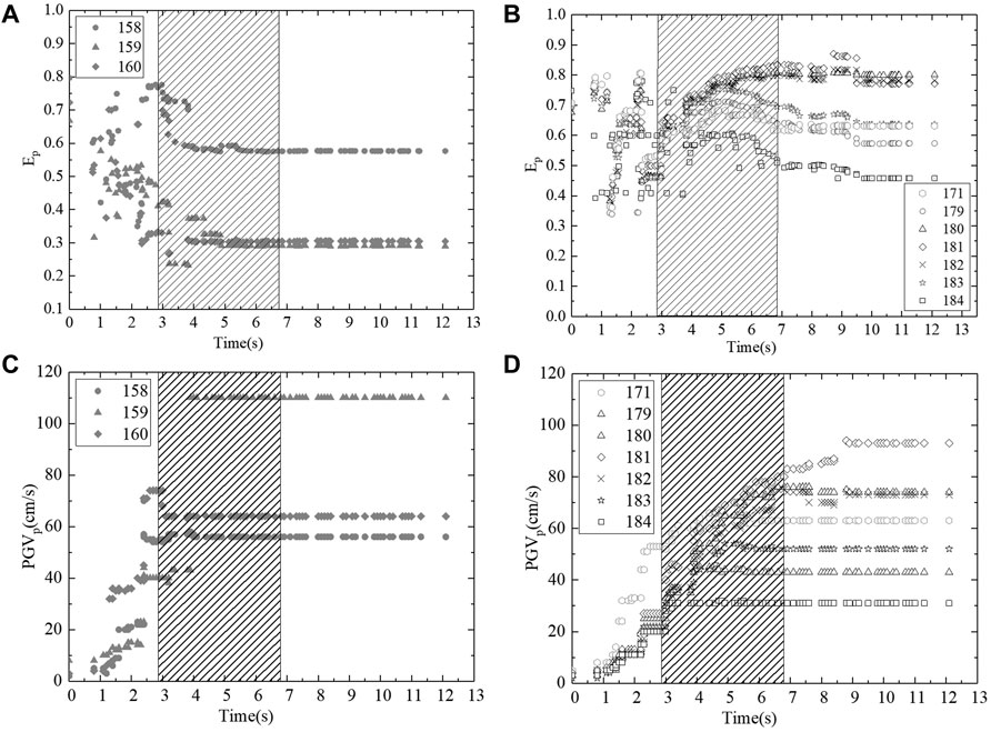
FIGURE 5. E_p values of final ground motions at (A) near-epicenter stations and (B) rupture-direction stations; and PGV_p values of final ground motions at (C) near-epicenter stations and (D) rupture-direction stations during the Imperial Valley Earthquake.

FIGURE 6

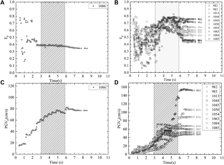
FIGURE 6. E_p values of final ground motions at (A) near-epicenter stations and (B) rupture-direction stations, and PGV_p values of final ground motions at (C) near-epicenter stations and (D) rupture-direction stations during the Northridge Earthquake.

In Figure 5A, at the near-epicenter stations, E_p varies during the initial rupture process and tends towards more constant values before and during the rupture of the asperity. In Figure 5B, at the rupture-direction stations, E_p exhibits an obvious upward trend during the asperity rupturing process as energy is released by the rupture of the asperity. The subsequent slightly downward of E_p at several stations may be related to adjustments in the pulse model. The PGV_p values exhibit a clear upward trend that eventually flattens out as the rupture process slows. In Figure 5C, at near-epicenter stations, the behavior of the PGV_p indicator is similar to that of E_p; after 3 s, the PGV_p values are mostly constant. In Figure 5D, at the rupture-direction stations, PGV_p increases throughout the asperity rupture process. As demonstrated, the spatial relationship between the asperity and the seismic station affects the timing of the pulse generation during rupturing on the sub-faults.

The slip distribution in the 1994 Northridge Earthquake is highly heterogeneous; it is modeled using one major asperity and one secondary asperity in the fault plane. The E_p and PGV_p indicators for ten rupture-direction stations and one near-epicenter station are shown in Figure 6.

At most rupture-direction stations, the results are similar to those of the 1979 Imperial Valley Earthquake (Figure 5), where the rupture of the major asperity causes the PGV_p values to increase and the E_p values to both rise and then fall slightly. At near-epicenter station RSN1086, which is located in the backward rupture propagation direction of the asperities, the PGV_p values surpass the PGV identification threshold before the asperity ruptured.

Based on the results shown in Figures 5, 6, asperity significantly affects pulse indicators E_p and PGV_p in both strike-slip and dip-slip events; as such, we conclude that asperity heavily influences the velocity pulse generation process. Because E_p is greater than 0.3 in the initial rupture process at most stations, we infer that PGV_p is the indicator that controls the identification of the velocity pulses.

Contribution of Sub-fault Ground Motions

By forward modeling with the low-frequency numerical simulation method, Luo et al. (2020); Luo et al. (2021) modeled the pulse-like ground motions in the 1979 Imperial Valley Earthquake and the 1999 ChiChi Earthquake. In addition to discovering that the velocity pulses somewhat depend on the seismic moment and the distribution characteristics of the asperity in the source model, they also found that the velocity pulses were more heavily influenced by shallow asperities than they were by deep asperities. Lin et al. (2019) determined that the velocity pulse behavior in the 2018 Hualian Earthquake was mainly caused by motion on a local sub-fault of the Milun fault. Because the time series we analyze ultimately represent the superposition of individual sub-fault motions, we decide to break out the contribution of each sub-fault motion to the PGV_p indicators observed in the final time series using Eq. 6:

$C_{PA}=\frac{v_{sub}\left(i\right)}{pg{v}_f}(6)$

where C_PA is the contribution of each sub-fault to the PGV_p (pulse amplitude) indicator of the final ground motion, pgv_f refers to the peak amplitude of the final motions, and v_sub(i) represents the PGV_p value when the ground motion on sub-fault i is added to the previous superimposed ground motions. The C_PA values for the 1979 Imperial Valley Earthquake (128 sub-faults) and the 1994 Northridge Earthquake (256 sub-faults) are shown in Figures 7A,B. In Figures 7A,B, the color of the squares represents the slip distribution, and the height of the bar graphs represents the C_PA value for each sub-fault motion. Because the amplitude of the sub-fault ground motions can be positive or negative, C_PA values can also be positive or negative. In this discussion, we focus on the absolute C_PA value for each sub-fault motion.

FIGURE 7

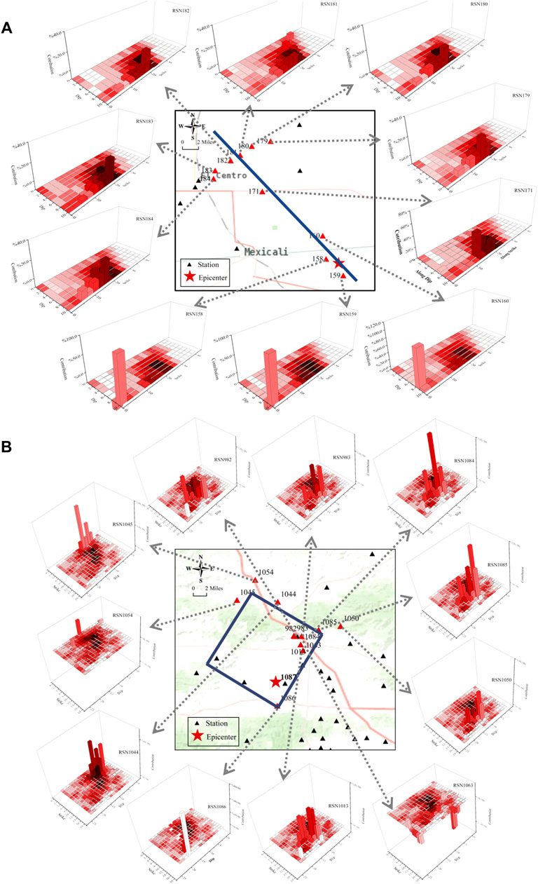
FIGURE 7. Contributions of the various sub-fault motions to the pulse amplitude in the final time series of (A) the Imperial Valley Earthquake and (B) the Northridge Earthquake.

In Figure 7A, at the near-epicenter stations, the absolute C_PA values are highest at the sub-faults closest to the rupture starting point; we attribute this observation to the large amount of energy released by the initial rupture of seismic source. Due to the proximity of the near-epicenter stations to the seismic source, the seismic waves arrive nearly instantaneously at the stations, resulting in velocity pulses that arrive early in the superposition process. At the rupture-direction stations, the magnitude of the final pulse amplitude is mainly composed of sub-fault ground motions at the asperity.

In Figure 7B, hanging-wall stations RSN982, RSN983, RSN1013, RSN1063, RSN1084, RSN1085, and RSN1050 are located close to the other asperity; as such, C_PA values from these stations are mainly caused by the rupture of the secondary asperity. At the stations with epicentral distances less than 20 km, the velocity pulses appear before the rupture of the major asperity. Because stations RSN1044, RSN1045, and RSN1054 are near the surface projection of the fault and are in the forward rupture propagation direction, the C_PA values at these stations come from the ground motion of several sub-faults after the rupture of the major asperity. At near-epicenter station RSN1086, sub-fault ground motions around the rupture initiation location contribute to the pulse amplitude. We also determine that the observed record at station RSN1087, which is located closest to the rupture initiation location, is a non-pulse-like ground motion. Site information from the USGS (http://www.usgs.gov) shows that V_s30 at RSN1087 is 257 m/s, by comparison, the V_s30 at pulse-like station RSN1086 is 495 m/s, which implies the softer site may absorb more energy.

Based on these results, we infer that pulse-like ground motion at the near-epicenter stations are mainly caused by the energy released during rupture initiation, while we attribute pulse-like ground motion at the rupture-direction stations to the rupture of the asperity; these observations are consistent with those of Poiata et al. (2017). Poiata et al. (2017) suggested that the seismic stations located in the forward fault rupture direction mainly affected the generation of pulse-like ground motions in the 2009 L’Aquila Earthquake (Italy). Overall, we conclude that the spatial relationship between the seismic stations and the asperities influences the pulse indicators produced during sub-fault ground motions, regardless of the fault type.

Effect of Slip Distribution on Pulse Indicators and Frequency Components

To further investigate the influence exerted by the asperity on the pulse-like ground motions, we run two sets of simulations: a simulation with a homogeneous slip distribution (i.e., without asperity) and a simulation with an inhomogeneous slip distribution (i.e., with asperities).

Pulse Indicator Results

In general, the rise time is positively correlated with the slip distribution in the seismic source model, which means that the rise time of the sub-faults at the asperity is longer. The rise time controls the pulse waveform and the pulse period, while the slip distribution affects the pulse amplitude. The asperity affects both the pulse period and pulse amplitude.

We used the F-K method to simulate 21 pulse-like ground motions from two types of slip distribution in the 1994 Northridge Earthquake and the 1979 Imperial Valley Earthquake. The similarity analysis described in Pulse Indicators in the Superposition of Sub-Fault Motions is applied to two types of simulated motions. The E_p and PGV_p results in the presence of these two types of slip distribution are shown in Figures 8, 9.

FIGURE 8

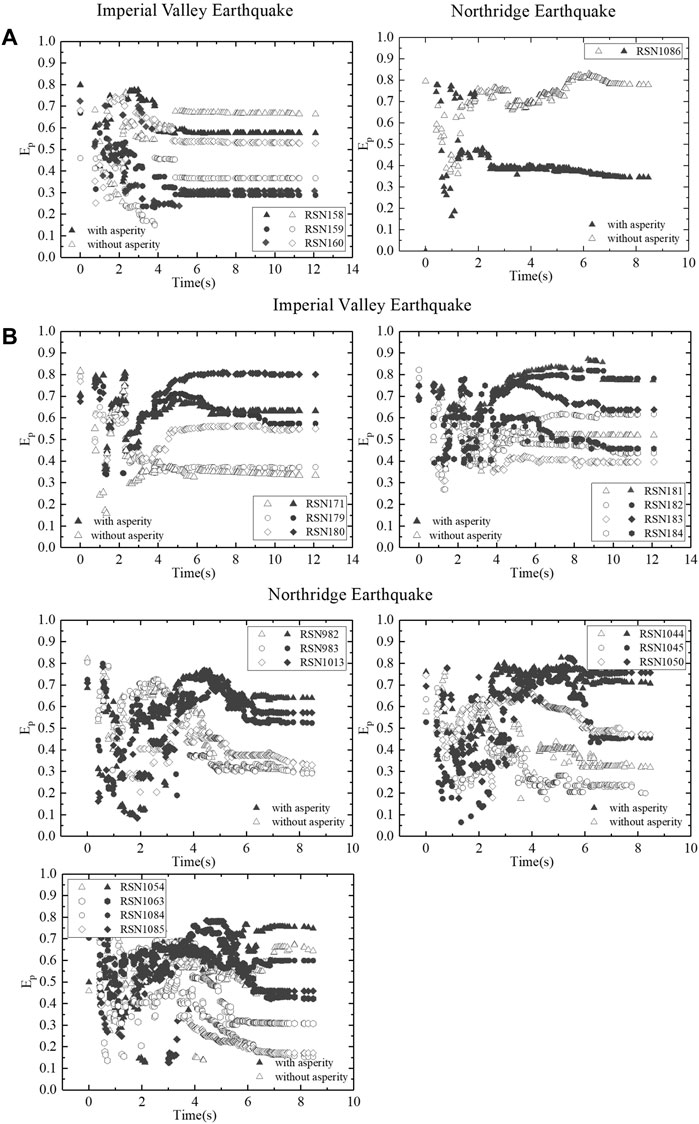
FIGURE 8. E_p values at (A) near-epicenter stations and (B) rupture-direction stations produced by homogenous and inhomogeneous slip distributions.

FIGURE 9

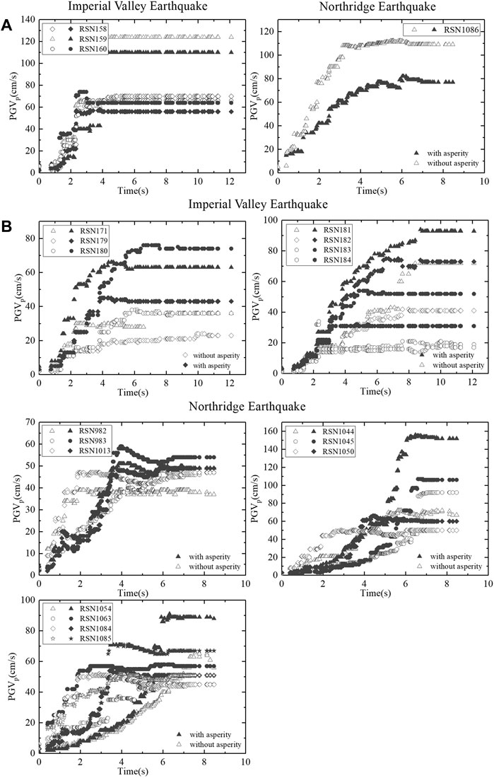
FIGURE 9. PGV_p values at (A) near-epicenter stations and (B) rupture-direction stations produced by homogenous and inhomogeneous slip distributions.

For the near-epicenter stations shown in Figure 8A, the E_p values from the homogeneous slip distribution simulation are significantly higher than those generated by the simulation with an inhomogeneous slip distribution. At the rupture-direction stations (Figure 8B), the E_p values from the inhomogeneous slip distribution simulation are higher than those from the homogeneous slip distribution simulation after the ground motions of the sub-faults at asperity are superimposed; thus, these waveforms are affected by the rupture of asperity (Figure 8B).

At the near-epicenter stations shown in Figure 9A, the PGV_p values from the homogeneous slip distribution simulation are higher than those of the inhomogeneous slip distribution model. However, at the rupture-direction stations (Figure 9B), the PGV_p values from the inhomogeneous slip distribution model are higher than those of the homogeneous slip distribution simulation, especially after the asperities rupture.

Figure 9B shows the PGV_p values for stations capturing time series. In the case of the 1994 Northridge Earthquake, the PGV_p values from the homogeneous slip distribution case are both higher (during the first 3 s) and lower (after the asperity ruptured) than those of the inhomogeneous slip distribution case. The phenomenon is not observed in the PGV_p values recorded during the 1979 Imperial Valley Earthquake. The PGV_p results from the dip-slip event are more complicated than those from the strike-slip event, especially during rupture initiation. Generally, in the case with an inhomogeneous slip distribution, the asperity exerts a stronger influence on the velocity pulses recorded at the rupture-direction stations; the initial rupture process is responsible for the larger pulse indicator values at the near-epicenter stations in the homogeneous slip distribution case.

Frequency Component Analysis

Both the fling-step effect and the directivity effect contribute to the low-frequency components of these pulse-like ground motions (Wang et al., 2013). Analysis of the time histories and spectrograms from backward-directivity and forward-directivity stations reveals that the energy captured at these two types of stations have different frequency components (Mena and Mai, 2011). The energy signatures from the forward-directivity stations primarily occur over a short time period, while the energy signatures recorded at the backward-directivity stations occur over the entire period.

The Windowed Fourier Transform results for the time series of the 1979 Imperial Valley Earthquake captured at two near-epicenter stations and two rupture-direction stations are shown in the top row and the bottom row of Figure 10, respectively.

FIGURE 10

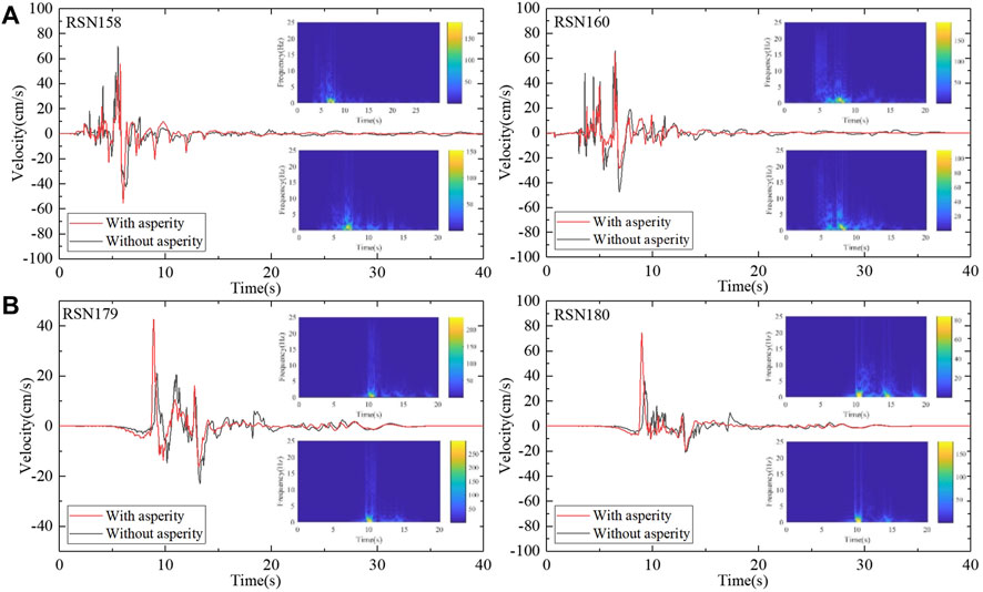
FIGURE 10. Velocity time histories and time-frequency spectra for (A) near-epicenter stations and (B) rupture direction stations. The red and the black lines represent the simulated velocity time histories from the inhomogeneous and homogeneous slip distributions, respectively. The diagram in the upper right-hand corner is the time-frequency analysis spectrum from a station with a time series generated by a homogeneous slip distribution and the diagram in the lower right-hand corner is the time-frequency analysis spectrum from a station with a time series generated by an inhomogeneous slip distribution. The color bar represents the amplitude of the Fourier spectra.

At near-epicenter stations RSN158 and RSN160, the low-frequency (0–1 Hz) energy of the ground motions generated by the homogeneous slip distribution is concentrated in a shorter time duration, and the Fourier spectral amplitude is higher than those produced by the inhomogeneous slip distribution. Furthermore, the PGV values from the homogeneous slip distribution case are higher than those generated by the inhomogeneous slip distribution scenario. At the rupture-direction stations RSN179 and RSN180, the low-frequency energy occupies shorter time duration than those from the inhomogeneous slip distribution and the PGV values produced by an inhomogeneous slip distribution are higher than those produced by the homogeneous slip distribution case. Our results suggest that at the near-epicenter stations, pulse indicators E_p and PGV_p for a homogeneous slip distribution are higher than those generated by an inhomogeneous slip distribution; the low-frequency pulse energy components are more pronounced and tend to occur over shorter time duration. The PGV values from the homogeneous slip distribution are larger than those generated by the inhomogeneous slip distribution. At the rupture-direction stations, both before and after the asperity ruptures, pulse indicators E_p and PGV_p have high values in the presence of an inhomogeneous slip distribution and pulse energy components that are composed of strong low frequency signals that occur over short time duration.

Conclusion

In this study, we investigate the generation mechanism of long-period velocity pulses. We simulate the near-fault ground motions in the 1979 Imperial Valley Earthquake (strike-slip event) and the 1994 Northridge Earthquake (dip-slip event) using the F-K method. To identify the velocity pulses in the time series produced by sub-fault ground motions, we apply the PPM model. By investigating the effect of the asperity, we demonstrate that pulse generation is related to the spatial relationship between the rupture starting point, the asperity, and the seismic station that captures the ground motion data. At the near-epicenter stations, pulse indicators E_p and PGV_p surpass the pulse identification threshold before the asperity ruptures. This observation indicates that the velocity pulses are generated by the significant amounts of energy released during the rupture initiation process. At the rupture-direction stations, the energy released by the rupture of the asperity contributes to the upward trend of the E_p and PGV_p values.

In both earthquakes, the pulse indicators increase when the asperity ruptures. By defining the contribution of each sub-fault ground motion to the pulse amplitude, we find that the amplitude of the velocity pulse at the near-epicenter stations largely consists of ground motion contributions from sub-faults located close to the rupture starting point. At the rupture-direction stations, in the case of a strike-slip fault, the pulse amplitude consists of ground motion contributions from sub-faults close to the asperity. In the case of a dip-slip fault, the pulse amplitude consists of ground motion contributions from sub-faults close to the major or secondary asperity after they rupture.

We also compare the pulse indicators and the frequency components in simulated ground motions from homogenous and inhomogeneous slip distributions. Our results suggest that, at near-epicenter stations, the pulse indicators produced by the homogeneous slip distribution are larger than those generated by the inhomogeneous slip distribution. Furthermore, the homogeneous slip distribution pulses mainly consist of low-frequency components that are emitted over short time duration. At the rupture-direction stations, the pulse indicators produced by an inhomogeneous slip distribution are larger than those generated by a homogeneous slip distribution. These inhomogeneous slip distribution pulses mainly consist of low-frequency components.

This investigation of the pulse generation mechanism and distribution characteristics can provide an analytical reference basis for the seismic design of engineering structures. In our future research, we will continue to explore other pulse identification methods and the mechanism of velocity pulses generation.

Data Availability Statement

The raw data supporting the conclusions of this article will be made available by the authors, without undue reservation.

Author Contributions

LH: Investigation, Calculation, Visualization, Writing Original Draft; ZT: Research Guidance, Supervision, Writing, Review and Editing. ZC: Research Data Curation and Validation XT: Research Guidance.

Funding

This research was financially supported by the Scientific Research Fund of Institute of Engineering Mechanics, China Earthquake Administration (Grant No. 2020B02), and the National Natural Science Foundation of China (No. 51678540, 51778197, and 51478443).

Conflict of Interest

The authors declare that the research was conducted in the absence of any commercial or financial relationships that could be construed as a potential conflict of interest.

Publisher’s Note

All claims expressed in this article are solely those of the authors and do not necessarily represent those of their affiliated organizations, or those of the publisher, the editors and the reviewers. Any product that may be evaluated in this article, or claim that may be made by its manufacturer, is not guaranteed or endorsed by the publisher.

Acknowledgments

Special thanks to reviewers for their careful work and thoughtful suggestions to improve this article. The strong ground motion data were downloaded from the Pacific Earthquake Engineering Research Center. The authors would like to thank Prof. Zhiwang Chang for providing the pulse-like ground motion identification algorithms.

References

Baker, J. W. (2007). Quantitative Classification of Near-Fault Ground Motions Using Wavelet Analysis. Bull. Seismological Soc. America 97, 1486–1501. doi:10.1785/0120060255

CrossRef Full Text | Google Scholar

Cao, Z. L. (2020). Synthesis of Three-Dimensional Broadband Strong Ground Motion Field Based on FK Approach. PhD thesis. Harbin, China: Harbin Institute of Technology. in Chinese.

Google Scholar

Cao, Z., Tao, X., Tao, Z., and Tang, A. (2019). Kinematic Source Modeling for the Synthesis of Broadband Ground Motion Using the F-K Approach. Bull. Seismol. Soc. Am. 109 (5), 1738–1757. doi:10.1785/0120180294

CrossRef Full Text | Google Scholar

Chang, Z. W., Luca, F. D., and Goda, K. (2020). “Characteristics of Near-Fault Acceleration Pulses and Implications on the Building Structures,” in Proceeding of 17th World Conference on Earthquake Engineering.

Google Scholar

Chen, X., and Wang, D. (2020). Multi-Pulse Characteristics of Near-Fault Ground Motions. Soil Dyn. Earthquake Eng. 137 (4), 106275. doi:10.1016/j.soildyn.2020.106275

CrossRef Full Text | Google Scholar

Dickinson, B. W., and Gavin, H. P. (2011). Parametric Statistical Generalization of Uniform-Hazard Earthquake Ground Motions. J. Struct. Eng. 137, 410–422. doi:10.1061/(asce)st.1943-541x.0000330

CrossRef Full Text | Google Scholar

Fayjaloun, R., Causse, M., Voisin, C., Cornou, C., and Cotton, F. (2017). Spatial Variability of the Directivity Pulse Periods Observed during an Earthquake. Bull. Seismological Soc. America 107 (1), 308–318. doi:10.1785/0120160199

CrossRef Full Text | Google Scholar

Fumal, T. E., Gibbs, J. F., and Roth, E. F. (1982). In-Situ Measurements of Seismic Velocity at 10 Strong Motion Accelerograph Stations in Central California. J. Syn. Org. Chem. Jpn. 30, 992–1005. doi:10.5059/yukigoseikyokaishi.30.992

CrossRef Full Text | Google Scholar

Graves, R. W., and Pitarka, A. (2010). Broadband Ground-Motion Simulation Using a Hybrid Approach. Bull. Seismological Soc. America 100 (5A), 2095–2123. doi:10.1785/0120100057

CrossRef Full Text | Google Scholar

Hartzell, S., Guatteri, M., Mai, P. M., Liu, P. C., and Fisk, M. (2005). Calculation of Broadband Time Histories of Ground Motion, Part II: Kinematic and Dynamic Modeling Using Theoretical Green's Functions and Comparison with the 1994 Northridge Earthquake. Bull. Seismological Soc. America 95 (2), 614–645. doi:10.1785/0120040136

CrossRef Full Text | Google Scholar

Hartzell, S., Frankel, A., Liu, P., Zeng, Y., and Rahman, S. (2011). Model and Parametric Uncertainty in Source-Based Kinematic Models of Earthquake Ground Motion. Bull. Seismological Soc. America 101 (5), 2431–2452. doi:10.1785/0120110028

CrossRef Full Text | Google Scholar

Hartzell, S., and Heaton, T. H. (1983). Inversion of Strong Ground Motion and Teleseismic Waveform Data for the Fault Rupture History of the 1979 Imperial Valley, California, Earthquake. Bull. Seismol. Soc. Am. 73 (6), 1553–1583. doi:10.1785/BSSA07306A1553

CrossRef Full Text | Google Scholar

Heaton, T. H., Hall, J. F., Wald, D. J., and Halling, M. W. (1995). Response of High-Rise and Base-Isolated Buildings to a Hypothetical M W 7.0 Blind Thrust Earthquake. Science 267, 206–211. doi:10.1126/science.267.5195.206

PubMed Abstract | CrossRef Full Text | Google Scholar

Huang, N. E., Shen, Z., Long, S. R., Wu, M. C., Shih, H. H., Zheng, Q., et al. (1998). The Empirical Mode Decomposition and the Hilbert Spectrum for Nonlinear and Non-stationary Time Series Analysis. Proc. R. Soc. Lond. A. 454, 903–995. doi:10.1098/rspa.1998.0193

CrossRef Full Text | Google Scholar

Jiang, L. J., and Bai, G. L. (2016). Study on Energy Characteristics of Different Types of Near-Fault Pulse Ground Motions. J. Struct. Eng. 32, 92–96. (in Chinese).

Google Scholar

Joyner, W. B., Warrick, R. E., and Fumal, T. E. (1981). The Effect of Quaternary Alluvium on Strong Ground Motion in the Coyote Lake, California, Earthquake of 1979. Bull. Seismol. Soc. Am. 71 (4), 1333–1349. doi:10.1007/BF01240590

CrossRef Full Text | Google Scholar

Kagawa, T. (2009). “Conditions of Fault Rupture and Site Location that Generate Damaging Pulse Waves,” in Proceedings of the 6th International Conference on Urban Earthquake Engineering.

Google Scholar

Lin, Y. Y., Kanamori, H., Zhan, Z. W., Ma, K. F., and Yeh, T. Y. (2019). Modelling of Pulse-like Velocity Ground Motion during the 2018 M_w 6.3 Hualien Earthquake, Taiwan. Geophys. J. Int. 223 (1), 348–365. doi:10.1093/gji/ggaa306

CrossRef Full Text | Google Scholar

Liu, Q. F. (2005). Studies on Near-Fault Ground Motions Based on Kinematic and Dynamic Source Models. PhD thesis. Harbin, China: Institute of Engineering Mechanics, China Earthquake Administration. (in Chinese).

Google Scholar

Luo, Q. B. (2019). Studies on Numerical Simulation of Near-Fault Large Velocity Pulse Based on Kinematic Source Model. Master Dissertation. Beijing, China: Institute of Geophysics, China Earthquake Administration. (in Chinese).

Google Scholar

Luo, Q. B., Dai, F., Liu, Y., and Chen, X. L. (2020). Simulating the Near-Field Pulse-like Ground Motions of the Imperial Valley, California Earthquake. Soil Dynam. Earthq. Eng. 138, 106–347. doi:10.1016/j.soildyn.2020.106347

CrossRef Full Text | Google Scholar

Luo, Q., Dai, F., Liu, Y., Gao, M., Li, Z., and Jiang, R. (2021). Seismic Performance Assessment of Velocity Pulse-like Ground Motions under Near-Field Earthquakes. Rock Mech. Rock Eng. 54, 3799–3816. doi:10.1007/s00603-021-02475-2

CrossRef Full Text | Google Scholar

Mavroeidis, G. P., and Papageorgiou, A. S. (2003). A Mathematical Representation of Near-Fault Ground Motions. Bull. Seismological Soc. America 93 (3), 1099–1131. doi:10.1785/0120020100

CrossRef Full Text | Google Scholar

Mena, B., and Mai, P. M. (2011). Selection and Quantification of Near-Fault Velocity Pulses Owing to Source Directivity. Georisk: Assess. Manag. Risk Engineered Syst. Geohazards 5 (1), 25–43. doi:10.1080/17499511003679949

CrossRef Full Text | Google Scholar

Mimoglou, P., Psycharis, I. N., and Taflampas, I. M. (2014). Explicit Determination of the Pulse Inherent in Pulse-like Ground Motions. Earthquake Engng Struct. Dyn. 43, 2261–2281. doi:10.1002/eqe.2446

CrossRef Full Text | Google Scholar

Miyake, H., Iwata, T., and Irikura, K. (2001). Estimation of Rupture Propagation Direction and Strong Motion Generation Area from Azimuth and Distance Dependence of Source Amplitude Spectra. Geophys. Res. Lett. 28 (14), 2727–2730. doi:10.1029/2000GL011669

CrossRef Full Text | Google Scholar

Miyake, H., Iwata, T., and Irikura, K. (2003). Source Characterization for Broadband Ground-Motion Simulation: Kinematic Heterogeneous Source Model and Strong Motion Generation Area. Bull. Seismological Soc. America 93, 2531–2545. doi:10.1785/0120020183

CrossRef Full Text | Google Scholar

Poiata, N., Miyake, H., and Koketsu, K. (2017). Mechanisms for Generation of Near-Fault Ground Motion Pulses for Dip-Slip Faulting. Pure Appl. Geophys. 174, 3521–3536. doi:10.1007/s00024-017-1540-z

CrossRef Full Text | Google Scholar

Porcella, R. L. (1984). Geotechnical Investigations at Strong-Motion Stations in the Imperial Valley. California: U.S. Geological Survey. doi:10.3133/ofr84562

CrossRef Full Text | Google Scholar

Scala, A., Festa, G., and Del Gaudio, S. (2018). Relation between Near-Fault Ground Motion Impulsive Signals and Source Parameters. J. Geophys. Res. Solid Earth 123, 7707–7721. doi:10.1029/2018JB01563

CrossRef Full Text | Google Scholar

Shahi, S. K., and Baker, J. W. (2011). An Empirically Calibrated Framework for Including the Effects of Near-Fault Directivity in Probabilistic Seismic Hazard Analysis. Bull. Seismological Soc. America 101 (2), 742–755. doi:10.1785/0120100090

CrossRef Full Text | Google Scholar

Shahi, S. K., and Baker, J. W. (2014). An Efficient Algorithm to Identify Strong-Velocity Pulses in Multicomponent Ground Motions. Bull. Seismological Soc. America 104 (5), 2456–2466. doi:10.1785/0120130191

CrossRef Full Text | Google Scholar

Sharbati, R., Rahimi, R., Koopialipoor, M. R., Elyasi, N., Khoshnoudian, F., Ramazi, H. R., et al. (2020). Detection and Extraction of Velocity Pulses of Near-Fault Ground Motions Using Asymmetric Gaussian Chirplet Model. Soil Dynam. Earthq. Eng. 133, 106–123. doi:10.1016/j.soildyn.2020.106123

CrossRef Full Text | Google Scholar

Somerville, P. G. (2003). Magnitude Scaling of the Near Fault Rupture Directivity Pulse. Phys. Earth Planet. 137 (1-4), 201–212. doi:10.1016/S0031-9201(03)00015-3

CrossRef Full Text | Google Scholar

Somerville, P. G., Smith, N. F., Graves, R. W., and Abrahamson, N. A. (1997). Modification of Empirical Strong Ground Motion Attenuation Relations to Include the Amplitude and Duration Effects of Rupture Directivity. Seismological Res. Lett. 68 (1), 199–222. doi:10.1785/gssrl.68.1.199

CrossRef Full Text | Google Scholar

Somerville, P., Irikura, K., Graves, R., Sawada, S., Wald, D., Abrahamson, N., et al. (1999). Characterizing Crustal Earthquake Slip Models for the Prediction of Strong Ground Motion. Seismological Res. Lett. 70 (1), 59–80. doi:10.1785/gssrl.70.1.59

CrossRef Full Text | Google Scholar

Tang, Y., Wu, C., and Wu, G. (2021). Automated Detection of Velocity Pulses in Ground Motions Based on Adaptive Similarity Search in Response Spectrum. Soil Dyn. Earthquake Eng. 149, 106626. doi:10.1016/j.soildyn.2021.106626

CrossRef Full Text | Google Scholar

Tsuda, K. (2020). “Possible Mechanisms of Generating Velocity Pulses Observed on the Nishihara Village during the 2016 Kumamoto Earthquake M_j 7.3,” in Proceeding of the 17th World Conference on Earthquake Engineering.

Google Scholar

Wald, D. J., Heaton, T. H., and Hudnut, K. W. (1996). The Slip History of the 1994 Northridge, California, Earthquake Determined from Strong-Motion, Teleseismic, GPS, and Leveling Data. Bull. Seismol. Soc. Am. 86 (1B), S49–S70. doi:10.1029/95JB03253

CrossRef Full Text | Google Scholar

Wang, B., Bai, G. L., Wang, C. Q., and Dai, H. J. (2013). Comparative Study on Energy Time-Frequency Distribution of Long-Period Ground Motions Based on Hilbert-Huang Transform. Earthq. Eng. Eng. Vib. 33 (3), 71–80. doi:10.11810/1000-1301.20130310

CrossRef Full Text | Google Scholar

Wang, H. Y. (2004). Finite Fault Source Model for Predicting Near-field Srong Ground Motion. PhD thesis. Harbin (China): Institute of Engineering Mechanics, China Earthquake Administration.

Google Scholar

Whitney, R. (2019). Quantifying Near Fault Pulses Using Generalized Morse Wavelets. J. Seismol 23, 1115–1140. doi:10.1007/s10950-019-09858-7

CrossRef Full Text | Google Scholar

Xu, Z., and Agrawal, A. (2010). Decomposition and Effects of Pulse Components in Near-Field Ground Motions. J. Struct. Eng. 136, 690–699. doi:10.1061/(ASCE)ST.1943-541X.0000122

CrossRef Full Text | Google Scholar

Zhai, C., Chang, Z., Li, S., Chen, Z., and Xie, L. (2013). Quantitative Identification of Near-Fault Pulse-like Ground Motions Based on Energy. Bull. Seismological Soc. America 103 (5), 2591–2603. doi:10.1785/0120120320

CrossRef Full Text | Google Scholar

Zhu, L., and Rivera, L. A. (2002). A Note on the Dynamic and Static Displacements from a Point Source in Multilayered Media. Geophys. J. Int. 148 (3), 619–627. doi:10.1046/j.1365-246X.2002.01610.x

CrossRef Full Text | Google Scholar