 Bin Huang1
 Jin Zhang
 Chenghu Sun
- 1National Meteorological Center, China Meteorological Administration, Beijing, China
- 2CMA Earth System Modeling and Prediction Centre (CEMC), Beijing, China
- 3State Key Laboratory of Severe Weather, Chinese Academy of Meteorological Sciences, Beijing, China
- 4State Key Laboratory of Severe Weather and Institute of Climate System, Chinese Academy of Meteorological Sciences, Beijing, China
- 5Collaborative Innovation Center on Forecast and Evaluation of Meteorological Disasters, Nanjing University of Information Science and Technology, Nanjing, China
Based on the operational version of the China Meteorological Administration Typhoon Model (CMA-TYM, formerly known as GRAPES_TYM), a series of numerical tests are conducted by optimizing the boundary layer parameterization scheme, vertical resolution, and boundary conditions. Instead of the sea surface temperature (SST) from the Global Forecast System (GFS) model, more accurate daily SST data reflecting the daily SST variation are used as the boundary condition. The new SST dataset is capable of representing the key points in the area, including the low coastal SST related to upwelling, the intrusion of the Yellow Sea (YS) Warm Current, and the ocean front between the YS and the East China Sea. An analysis of the performances of two boundary layer parameterization schemes (the Yonsei University scheme and the Medium-Range Forecast scheme) in characterizing turbulent heat exchange reveals that the former can more accurately reflect offshore turbulence and forecast the fog area. By increasing the number of vertical layers of the model to 68 and reducing the height of the bottom layer to approximately 10 m, the model presents a better performance in simulating the rapid formation and dissipation of sea fog. With the above improvements, the equitable threat score (ETS) for the hindcasting of eleven sea fog cases in the spring of 2018 increases by 61%, mainly due to the increase in the correctly forecasted fog area.
Introduction
Sea fog is a phenomenon in which water vapour condenses in the lower atmosphere over the sea (including shores and islands) under the influence of the ocean (Wang, 1983). In recent years, the casualties and property losses caused by sea fog have gradually approached those caused by extreme weather events, such as typhoons and tornadoes (Gultepe et al., 2007). The offshore waters of China are characterized by one of the highest frequencies of sea fog occurrence worldwide; here, this phenomenon arises due to the strong sea temperature gradient and poses serious hazards to the economic development and social security of coastal China. If the occurrence, duration, extent of influence and concentration of sea fog could be accurately predicted by an operational department, early warnings could be provided, and thus, corresponding emergency measures could be taken to reduce and avoid losses.
However, as a weather phenomenon influenced by a weak pressure field, sea fog is difficult to be numerically predicted. The formation and development of sea fog are affected by a series of dynamic and thermodynamic processes, such as synoptic circulations, air-sea heat and water vapour exchanges, boundary layer turbulence and entrainment, and long-wave and shortwave radiation. In particular, one of the most important mechanisms responsible for the formation of sea fog is the condensation caused by the cooling of warm and humid air advecting to the cold sea surface. In some early attempts to numerically simulate sea fog, many scholars employed mesoscale forecasting models (Ballard et al., 1991; Golding, 1993; Nakanishi, 2000; Pagowski et al., 2004; Koračin et al., 2005). Mesoscale models have been used to simulate the formation of sea fog in China since the turn of the century, and the corresponding mechanisms have been investigated (Fu et al., 2004; Fu et al., 2006; Fu et al., 2008; Wang et al., 2012; Cheng et al., 2013; Huang et al., 2015; Huang et al., 2019). Focusing on ten cases of sea fog over the Yellow Sea (YS) in spring, Lu et al. (2014) carried out a sensitivity study on the parameterization schemes of the Weather Research and Forecasting (WRF) model and found that the best combination of the boundary layer scheme and the microphysical scheme comprises the Yonsei University (YSU) scheme and the Purdue Lin scheme, respectively. Based on the simulation of fog over the YS through the WRF model, Yang and Gao (2016) reported that increasing the vertical resolution could significantly improve the ability to forecast the horizontal fog area. In addition, the quality of the initial field is essential for sea fog forecasts and can be improved by assimilating multi-source observation data, which also helps improve the forecasting skill (Gao et al., 2010a; Gao et al., 2010b; Wang and Gao, 2016; Gao and Gao, 2019).
Compared with the rapid development in other research aspects of atmospheric science, the operational application of a numerical prediction technique for sea fog in China is still in its infancy. National Meteorological Center of China and meteorological services in coastal provinces and cities have gradually established a numerical prediction system for sea fog in recent years based on imported regional models such as the WRF and the Regional Atmospheric Modeling System (RAMS) to develop related forecast products, which can provide certain support for operational forecasts (Huang et al., 2014). In the operations of national marine meteorological forecasts, the continuously improving the China Meteorological Administration Typhoon Model (CMA-TYM, formerly known as GRAPES_TYM) has become an important reference for meteorological departments to forecast marine weather (Ma and Chen, 2018, Ma et al., 2018, Zhang et al., 2017). However, CMA-TYM was originally developed for the numerical prediction of tropical cyclones. Sea fog prediction is only its by-product and has not been carefully evaluated. In order to improve its sea fog forecast skill, the description of the marine boundary layer closely related to the formation and evolution of sea fog in CMA-TYM needs to be further refined. Therefore, this study intends to improve the simulation and prediction of sea fog by CMA-TYM to support controllable operational forecasts in China.
Data, Method and Model Description
Data
The background field uses 3-hourly data with a resolution of 0.5°×0.5° and 26 vertical layers from the Global Forecast System (GFS) produced by the National Centers for Environmental Prediction (NCEP), and multi-source observation data are assimilated for the initial field. Another sea surface temperature (SST) dataset used in the forecast is composed of daily SST data with a resolution of 0.25°×0.25° produced by the North-East Asian Regional Global Ocean Observing System (NEAR-GOOS).
Due to the lack of the routine observations over the sea, satellite images with high spatial and temporal resolution have already been used as an important approach to monitor the process of sea fog evolution (e.g., Wu et al., 2015; Wang et al., 2018). The satellite cloud images employed for the retrieval of sea fog are based on high-resolution infrared brightness temperature and visible albedo data obtained by the Japanese Himawari-8 geostationary satellite, and the SST data used for the retrieval originate from the NCEP reanalysis product. In the paper, we adopt the retrieval method proposed by Wang et al. (2015), which was proved feasible by comparison with observation data in the offshore areas of China, to provide sea fog retrievals to verify model forecasts. For convenience, we refer to such retrieval data as observations below.
CMA-TYM
The model domain utilized in current operational forecasts is shown in Figure 1, which uses an equal-latitude and equal-longitude grid system with a horizontal resolution of 0.09°×0.09° and 50 vertical layers with a height-based terrain-following coordinate. The purpose of this study is to improve the framework of operational forecasts by CMA-TYM. Therefore, although such a large area is not required to forecast sea fog in the offshore waters of China, this domain is used to conduct the numerical experiment in this study. Other specifications of the model parameters are shown in Table 1.
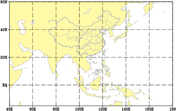
FIGURE 1. Simulation domain of CMA-TYM.
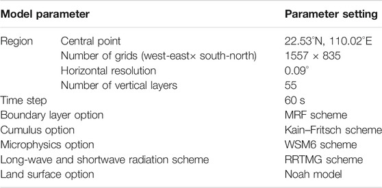
TABLE 1. Parameter settings of CMA-TYM.
Model Diagnostic Methods of Sea Fog
When visible light travels through the air, it is scattered and blocked by suspended liquid and solid particles. The extinction coefficient can be used to comprehensively reflect the weakening effect of air on light. Assuming that the air near the observation point is homogeneous, the extinction coefficient is constant. According to Koschmieder’s law, the calculation formula for horizontal visibility is as follows:
where
where
Nevertheless, we cannot determine whether the bottom of sea fog is decoupled from the sea surface (thereby becoming a low-level stratus cloud) since satellite monitoring is employed to determine the fog area at sea regardless of whether a subjective or objective method is used. If the structure of stratus clouds (condensation is present at low altitudes but not at the bottom of the model) can be accurately predicted by the model but stratus clouds are treated as sea fog in satellite observations, the forecasted fog area is seriously underestimated when the liquid water content at the bottom of the model domain is compared with that observed within the fog area. To avoid this error, forecasted low-level stratus clouds are regarded as sea fog, and the height of 500 m is taken as the threshold for the fog-top height since the thickness of advecting fog over the YS generally does not exceed 400 m (Zhou and Du, 2010). Therefore, the forecasted fog area should meet the following criteria simultaneously: first, in model layers where the height ≤500 m, at least one layer is characterized by
Figure 2 shows several typical cases regarding the diagnosis of sea fog in the model. In the case shown in Figure 2A, condensed water particles stretch from the first layer
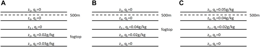
FIGURE 2. Diagnosis of the fog-top heights corresponding to three kinds of cloud water distributions. (A-C) See text for details.
Evaluation Methods
To quantitatively assess the forecast results, a point-to-point comparison is made based on the gridded sea fog forecasts and the observed fog areas. The numbers of grid points in the observation area and forecasted fog area are set as
where
Model Improvement Scheme
Improved Bottom Boundary Condition
Studies have shown that the bottom boundary conditions, especially the SST distribution, are important factors affecting the formation and development of sea fog (Fu et al., 2016). When warm and humid air advects to the cold sea surface, the initial heat exchange originates at the air-sea interface: heat is transferred to the ocean from the air near the sea surface (below a height of 1 m), and the region in which the temperature decreases extends upward under the influence of atmospheric turbulence, which affects the offshore layer (below a height of 10 m) and the boundary layer. Therefore, sea fog is triggered by warm, humid air and a cold sea surface. According to a sensitivity test of large-scale sea fog (figure omitted), when the offshore SST increases by 1 K, the forecasted fog area shrinks by tens of thousands of square kilometres. Furthermore, the SST near the shore may be lower than that of the open sea under the action of coastal upwelling, which creates favourable conditions for the formation of coastal sea fog.
At present, the SST field used in operational forecasts by CMA-TYM is entirely derived from global GFS data, which are updated every 3 h. However, the coarse grid of the GFS product is insufficient for sea fog forecasts. Therefore, daily SST data with a resolution of 0.25°×0.25° from NEAR-GOOS are used in this study; these data have been assimilated with multi-source observation data and are updated daily and thus are suitable for operational forecasts. However, the SST field from NEAR-GOOS is a daily average; hence, the daily variation trend is excluded. Therefore, the NEAR-GOOS SST is considered as the background field. The result of superimposing the NEAR-GOOS SST onto the daily variation trend of the GFS SST is taken as the SST boundary conditions for driving CMA-TYM. Both types of data are interpolated to the grids of CMA-TYM with 0.09°×0.09° horizontal resolution before superimposing. The new SST boundary condition of CMA-TYM is expressed as:
where
Figure 3 plots the SST distributions at 1200 UTC on April 18, 2018, before and after the inclusion of the NEAR-GOOS SST. The bottom boundary conditions before and after the addition of NEAR-GOOS SST data are roughly the same in the subtropical western Pacific. Specifically, in the Bohai Sea, the improved SST is approximately 0.5°C higher. In the central YS, the improved SST appears as a strong warm ridge. The low temperatures of the coastal waters on both sides of this warm ridge strengthen the temperature gradients, whereas the distribution of the GFS SST alone is smoother. The improved SST better reflects the tributaries of the Kuroshio Extension in the offshore waters of China, making it easier for the model to predict the occurrence of sea fog near the Shandong Peninsula, the coast of Jiangsu, and the Korean Peninsula, while sea fog is more difficult to forecast over the central YS due to the higher SST there. This result is basically consistent with the real situation; that is, sea fog in this area often appears over the eastern and western YS, while the central YS exhibits clear or cloudy skies. Moreover, a large number of ship observations have reported a strong sea temperature gradient (called an ocean front) at the junction between the YS and East China Sea (near 124°E, 30°N) in spring, which is accurately depicted by the improved SST.
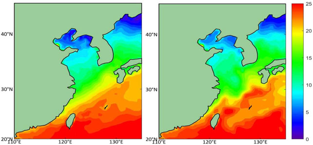
FIGURE 3. SST distributions (°C) at 1200 UTC on April 18, 2018. The left panel shows the GFS data, while the right panel shows the weighted average of the GFS and NEAR-GOOS data.
Improved Boundary Layer Scheme
The Medium-Range Forecast (MRF) boundary layer scheme, which has been thoroughly verified in forecasting the intensity and paths of typhoons, is used in operational forecasts by CMA-TYM. However, the MRF scheme may underestimate the turbulent mixing process when considering the entrainment process and the internal processes of the boundary layer together. Although this underestimation has little effect on severe weather processes such as typhoons and extratropical cyclones, the effect is unfavourable for sea fog forecasts. Numerical experiments on sea fog cases in the spring seasons of 2005–2011 show that the forecast results of the YSU scheme are better than those of the quasi-normal scale elimination, Mellor–Yamada and Mellor–Yamada–Nakanishi–Niino-2.5/3 models. However, no studies have compared the advantages and disadvantages of the YSU scheme with those of the MRF scheme. Therefore, comparative experiments for these two schemes are carried out in this study.
Taking an offshore sea fog case from April 19 to April 20, 2018, as an example, the MRF scheme and the YSU scheme are separately set as the boundary scheme, and the experiments are correspondingly denoted Exp-MRF and Exp-YSU, respectively. The forecast initial time is set to 1200 UTC on April 19. Figure 4 presents a comparison between the forecast results and observations. This sea fog was produced by southerly wind behind a high-pressure system; the fog began to form over the offshore sea surface and gradually developed upward due to the low SST of the coastal waters. During the day on April 20, the land cyclone system moved eastward, and the southwesterly wind strengthened; the sea fog stretched to the northeast and then weakened and disappeared due to solar radiation. Sea fog did not appear within 12 h in the Exp-MRF forecasts until a small area of sea fog appeared at 0300 UTC on April 20, which then quickly dissipated. In the Exp-YSU forecasts, a large area of fog formed on the night of April 19, and the forecast results were relatively close to the observations until 0300 UTC on April 20. Although Exp-YSU does not capture the dissipation well in the later stage of the forecasts, its forecast results are significantly better than those of Exp-MRF in general.
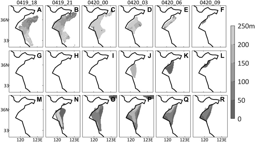
FIGURE 4. Comparison between the forecasted fog-top height and retrieved fog-top height from 1800 UTC on April 19 to 0600 UTC on April 20, 2018, from the (A–F) retrieval, (G–L) Exp-MRF and (M–R) Exp-YSU.
Table 2 shows the comprehensive scores of the two tests. For the MRF scheme, the
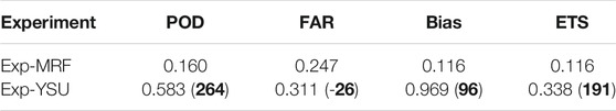
TABLE 2. Scores of the fog area (the number in brackets is the percentage by which the forecast results using the YSU scheme are improved compared with those using the MRF scheme).
Figure 5 shows that due to the weak turbulent mixing in the MRF scheme, the low-temperature air mass below 13°C always accumulates near the offshore surface (below a height of 50 m). However, in the YSU scheme, higher air masses are affected by the cooling of the offshore surface, and the region with a temperature below 13°C extends up to a height of 100 m. This intense cooling process in Exp-YSU facilitates the condensation of water vapour, and thus, the simulated fog area is larger than that in Exp-MRF.
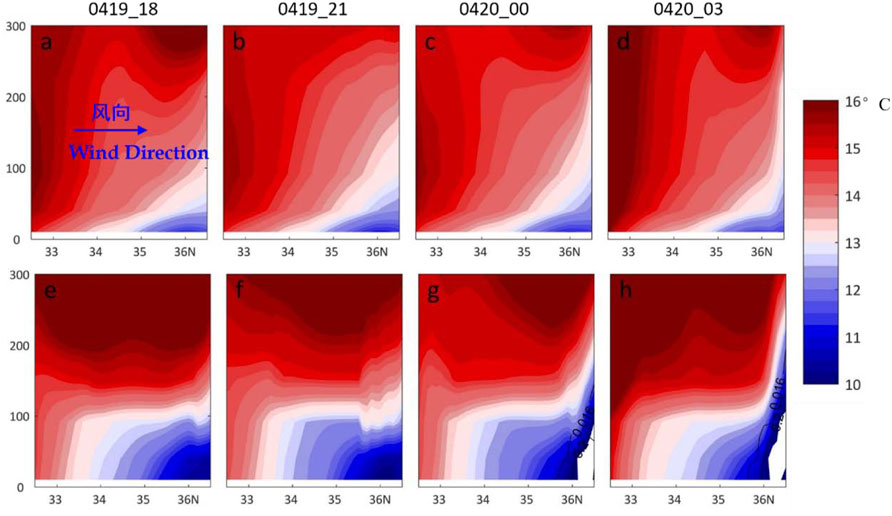
FIGURE 5. Temporal variation in the forecast results of (A–D) Exp-MRF and (E–H) Exp-YSU on the meridional vertical section along 121.5°E. The shading represents the temperature (unit: °C), and the contours represent the cloud-water mixing ratio (unit: g kg−1).
Improved Vertical Resolution
The vertical resolution determines the model accuracy in depicting vertical motions within the atmosphere and energy exchange and material exchange processes. For sea fog forecasting, a finer vertical resolution means more model layers in the boundary layer, which is conducive to the turbulent transfer of heat between layers. However, increasing the number of layers also means reducing the height of the bottom layer (
where
To compare the forecasts of the two schemes for the sea fog case during April 19–20, the experiments adopt two vertical resolutions of 50 layers and 68 layers, and the experiments are correspondingly denoted Exp-50 and Exp-68, respectively. The forecast initial time is set to 1200 UTC on April 19.
Figure 6 presents a comparison between the forecasts and observations. The increasing vertical resolution increases the fog area around the 12-h forecast. The improved trend is similar to that in the YSU scheme but weaker (Figure 4). It is worth noting that in the late forecast period, the fog dissipates faster in Exp-68 than in Exp-50. At 0600 UTC on April 20, the fog area forecasted in Exp-68 is much larger than that in Exp-50. After only 3 h, the fog area in Exp-68 is almost as large as that in Exp-50 since the lower height of
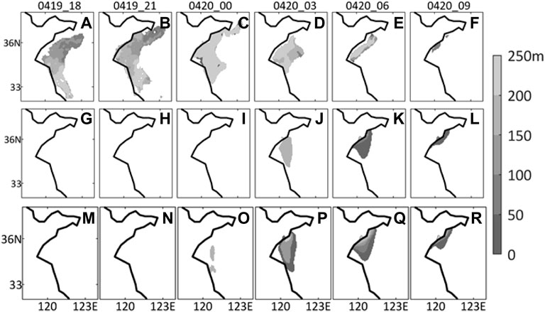
FIGURE 6. Comparison between the forecasted fog-top height and retrieved fog-top height from 1800 UTC on April 19 to 0600 UTC on April 20, 2018, from the (A–F) retrieval, (G–L) Exp-50 and (M–R) Exp-68.
Table 3 further shows the comprehensive scores of the two experiments. Compared with those of Exp-50, the
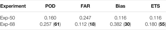
TABLE 3. Scores of the fog area (the number in brackets is the percentage by which the results of EXP-68 are improved compared to those of EXP-50).
The meridional cross-section along 121°E is plotted in Figure 7. In Exp-68, the temperature drops significantly below a height of 300 m, while the upper bound of the region with a temperature below 13°C increases in height. After the fog area (cloud water content greater than 0.016 g kg−1) is formed, the long-wave radiation of liquid water particles causes rapid cooling inside the fog area. At 0300 UTC on April 20, the surface air temperature in Exp-68 at 36°N is approximately 2°C lower than that in Exp-50.
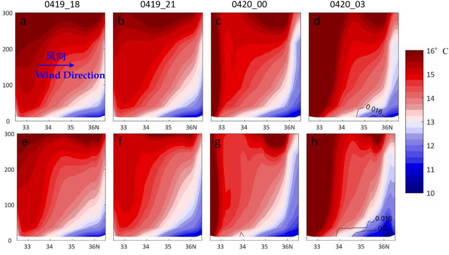
FIGURE 7. Temporal variation in the forecast results of (A–D) Exp-50 and (E–H) Exp-68 on the meridional vertical section along 121°E. The shading represents the temperature (unit: °C), and the contours represent the cloud-water mixing ratio (unit: g kg−1).
Assessment of the Overall Improvement
With the above results, an improved scheme for the forecasting of sea fog by CMA-TYM is established. The first step is to use the daily NEAR-GOOS SST as the bottom boundary of the model; the second step is to adopt the YSU scheme as the boundary layer scheme; and the third step is to increase the vertical resolution from 50 to 68 layers. To assess the overall improvement effect, simulation-based forecasts are carried out for eleven sea fog cases in the spring of 2018 (Table 4). The forecast initial time is set to 1200 UTC on the day before, and the lead time is 24 h. To compare the difference in the forecast effect before and after the improvement, two groups of experiments are designed. Group-A is a control test that adopts the settings of the operational forecast before the improvement; Group-B applies the abovementioned improved schemes, while the remaining settings are exactly the same as those of Group A. Table 5 shows the specifications.
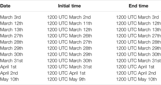
TABLE 4. Sea fog cases in the spring of 2018.

TABLE 5. Specifications of the control test and improvement test.
Table 6 lists the forecast scores of the eleven sea fog cases in the two groups. The forecasted fog area in Group-A is generally small. The
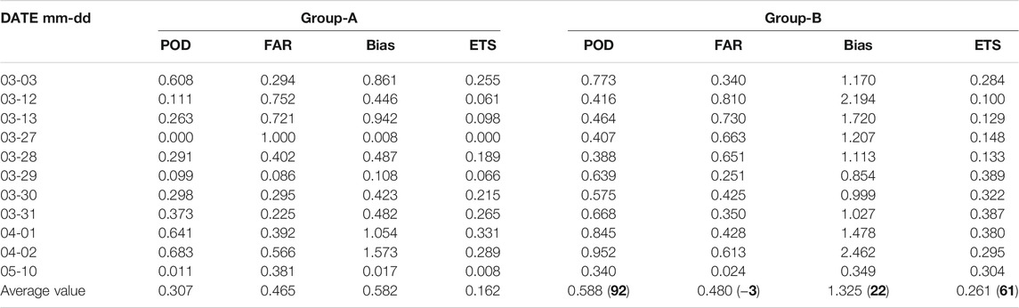
TABLE 6. Forecast scores (the number in brackets is the percentage of the improvement of Group-B over Group-A).
The forecasted fog area in Group-B is higher than that in Group-A due to the improved scheme, and the forecast scores of the former are better (except for the case on March 28). In particular, on May 10, the
Conclusion and Discussion
Based on the operational version of CMA-TYM, numerical experiments and improvement studies are carried out on sea fog forecasts regarding three aspects: the boundary layer scheme, the vertical resolution and the bottom boundary conditions. The main conclusions are as follows.
Highly precise and dynamic SST data are adopted as the bottom layer boundary conditions. The use of SST data can better reflect the low offshore SST caused by coastal upwelling, the temperature ridge in the middle of the YS, and the ocean front between the YS and the East China Sea. As the new boundary condition, these SST data are more conducive to improving the forecasting skills for sea fog.
Comparing the accuracies of the YSU scheme and MRF scheme in describing the turbulent heat exchange reveals that the former can more accurately reflect offshore turbulence and forecast the fog area.
A finer vertical resolution facilitates heat transfer simulation. Specifically, the lower bottom layer of the model is highly sensitive to changes in the SST and temperature of the overlying atmosphere, and this sensitivity is conducive to the rapid formation and dissipation of sea fog, thus correcting the current forecast error.
Through the improved scheme, the overall
After implementing these improvements, CMA-TYM is significantly improved in forecasting the extent of sea fog over the offshore water of China and thus can provide an important reference for operational forecasts. However, the current numerical forecast level for sea fog cannot fully satisfy the required accuracy of operational services due to the complexity of the structure and evolution of sea fog. Future models should be further improved by assimilating observational data from additional sources and developing regional air-ocean coupled models. In addition, the development of ensemble forecasts using multiple initial fields will be an important direction to reduce the uncertainties in sea fog forecasts.
Data Availability Statement
The raw data supporting the conclusion of this article will be made available by the authors, without undue reservation.
Author Contributions
BH: Formal analysis; Methodology and software; Writing–original draft. JZ: Supervision; Numerical Modeling. YC: Data curation. XG: Numerical Modeling. SM: Supervision. CS: Writing–review and editing.
Funding
This work was supported by the National Key Research and Development Program of China (2019YFC1510102, 2019YFC1510104).
Conflict of Interest
The authors declare that the research was conducted in the absence of any commercial or financial relationships that could be construed as a potential conflict of interest.
Publisher’s Note
All claims expressed in this article are solely those of the authors and do not necessarily represent those of their affiliated organizations, or those of the publisher, the editors and the reviewers. Any product that may be evaluated in this article, or claim that may be made by its manufacturer, is not guaranteed or endorsed by the publisher.
Acknowledgments
We thank the management and publishing organizations responsible for the NCEP GFS data, NCEP reanalysis data, NEAR-GOOS SST data, and Himawari-8 satellite data.
References
Ballard, S. P., Golding, B. W., and Smith, R. N. B. (1991). Mesoscale Model Experimental Forecasts of the Haar of Northeast Scotland. Mon. Wea. Rev. 119, 2107–2123. doi:10.1175/1520-0493(1991)119<2107:mmefot>2.0.co;2
Cheng, X. K., Cheng, H., Xu, J., and Ma, Y. J. (2013). Forming Reason of a Sea Fog Event and its Numerical Simulation over the Yellow Sea. J. Meteorology Environ. 29 (6), 15–23. (in Chinese). doi:10.3969/j.issn.1673-503X.2013.06.003
Fu, G., Li, P., Zhang, S., and Gao, S. H. (2016). A Brief Overview of the Sea Fog Study in China. Adv. Meteorol. Sci. Technol. 6 (2), 20–28. (in Chinese). doi:10.1016/0011-2275(95)95350-N
Fu, G., Wang, J. Q., Zhang, M. G., Guo, M. K., Guo, K. C., et al. (2004). An Observational and Numerical Study of a Sea Fog Event over the Yellow Sea on 11 April, 2004. Periodical Ocean Univ. China 34 (5), 720–726. (in Chinese). doi:10.1007/BF02873095
Fu, G., Guo, J., Pendergrass, A., and Li, P. (2008). An Analysis and Modeling Study of a Sea Fog Event over the Yellow and Bohai Seas. J. Ocean Univ. China 7 (1), 27–34. doi:10.1007/s11802-008-0027-z
Fu, G., Guo, J., Xie, S.-P., Duan, Y., and Zhang, M. (2006). Analysis and High-Resolution Modeling of a Dense Sea Fog Event over the Yellow Sea. Atmos. Res. 81, 293–303. doi:10.1016/j.atmosres.2006.01.005
Gao, S. H., Qi, Y. L., Zhang, S. B., et al. (2010a). Initial Conditions Improvement of Sea Fog Numerical Modeling over the Yellow Sea by Using Cycling 3DVAR Part I:WRF Numerical Experiments. Periodical Ocean Univ. China 40 (10), 001–009. (in Chinese).
Gao, S. H., Zhang, S. B., Qi, Y. L., and Gang, F. (2010b). Initial Conditions Improvement of Sea Fog Numerical Modeling over the Yellow Sea by Using Cycling 3DVAR Part Ⅱ:RAMS Numerical Experiments. Periodical Ocean Univ. China 40 (11), 001–010. (in Chinese). doi:10.3969/j.issn.1672-5174.2010.11.001
Gao, X. Y., and Gao, S. H. (2019). EnKF Assimilation of Cloud Water Path in Nowcasting Sea Fog over the Yellow Sea. Oceanologia Et Limnologia Sinica 50 (2), 248–260. (in Chinese). doi:10.11693/hyhz20181000243
Golding, B. W. (1993). A Study of the Influence of Terrain on Fog Development. Mon. Wea. Rev. 121, 2529–2541. doi:10.1175/1520-0493(1993)121<2529:asotio>2.0.co;2
Gultepe, I., Tardif, R., Michaelides, S. C., Cermak, J., Bott, A., Bendix, J., et al. (2007). Fog Research: A Review of Past Achievements and Future Perspectives. Pure Appl. Geophys. 164, 1121–1159. doi:10.1007/s00024-007-0211-x
Huang, B., Yan, L. F., Yang, C., and Xu, J. (2014). Development and marine Meteorological Numerical Prediction in China. Adv. Meteorol. Sci. Technol. 4 (3), 57–61. (in Chinese). doi:10.3969/j.issn.2095-1973.2014.03.010
Huang, H. J., Zhan, G. W., Liu, C. X., Tu, J., and Mao, W. K. (2015). A Case of Numerical Simulation of Sea Fog on the Southern China Coast. J. Trop. Meteorology 31 (5), 643–654. (in Chinese). doi:10.16032/j.issn.1004-4965.2015.05.007
Huang, S., Zhang, S. P., and Yi, L. (2019). The Analysis of the Formation of Coastal Fog under Surface Offshore Airflow in the Western Yellow Sea in spring. Periodical Ocean Univ. China 49 (6), 20–29. (in Chinese). doi:10.16441/j.cnki.hdxb.20180154
Koračin, D., Businger, J. A., Dorman, C. E., and Lewis, J. M. (2005). Formation, Evolution, and Dissipation of Coastal Sea Fog. Boundary-Layer Meteorology 117, 447–478. doi:10.1007/s10546-005-2772-5
Kunkel, B. A. (1984). Parameterization of Droplet Terminal Velocity and Extinction Coefficient in Fog Models. J. Clim. Appl. Meteorol. 23, 34–41. doi:10.1175/1520-0450(1984)023<0034:podtva>2.0.co;2
Lu, X., Gao, S. H., Rao, L. J., and Wang, Y. (2014). Sensitivity Study of WRF Parameterization Schemes for the spring Sea Fog in the Yellow Sea. J. Appl. Meteorol. Sci. 25 (3), 312–320. (in Chinese). doi:10.3969/j.issn.1001-7313.2014.03.008
Ma, S. H., and Chen, D. H. (2018). Performance of Regional Typhoon Model of National Meteorological Center. J. Trop. Meteorology 34 (4), 451–459. (in Chinese). doi:10.16032/j.issn.1004-4965.2018.04.002
Ma, S. H., Zhang, J., Shen, X., et al. (2018). The Upgrade of GRAPE_TYM in 2016 and its Impacts on Tropical Cyclone Prediction. J. Appl. Meterological Sci. 35 (3), 257–269. (in Chinese).
Nakanishi, M. (2000). Large-Eddy Simulation of Radiation Fog. Boundary-Layer Meteorology 94, 461–493. doi:10.1023/a:1002490423389
Pagowski, M., Gultepe, I., and King, P. (2004). Analysis and Modeling of an Extremely Dense Fog Event in Southern Ontario. J. Appl. Meteorol. 43, 3–16. doi:10.1175/1520-0450(2004)043<0003:aamoae>2.0.co;2
Wang, H., Zhang, Z., Liu, D., Yuan, C., Zhou, L., and Qian, W. (2018). Detection of Fog at Night by Using the New Geostationary Satellite Himawari-8[J]. Plateau Meteorology 37 (6), 17491764. (in Chinese). doi:10.7522/j.issn.1000-0534.2018.00037
Wang, S., Fu, D., Chen, D. L., Li, L. Y., and Fu, G. (2012). An Observation and Numerical Simulation of a Sea Fog Event over the Yellow Sea in the spring of 2009. Trans. Atmos. Sci. 35 (3), 282–294. (in Chinese). doi:10.1007/s11783-011-0280-z
Wang, Y. M., Gao, S. H., and Fu, G. (2015). Assimilating MTSAT-Derived Humidity in Nowcasting Sea Fog over the Yellow Sea. Weather Forecast. 29, 205–225. doi:10.1175/WAF-D-12-00123.1
Wang, Y. M., and Gao, S. H. (2016). Assimilation of Doppler Radar Radial Velocity in Yellow Sea Fog Numerical Modeling. Periodical Ocean Univ. China 46 (8), 1–12. (in Chinese). doi:10.16441/j.cnki.hdxb.20150361
Wu, X. J., Li, S. M., Liao, M., Cao, Z. Q., Wang, L., and Zhu, J. (2015). Analyses of Seasonal Feature of Sea Fog over the Yellow Sea and Bohai Sea Based on the Recent 20 Years of Satellite Remote Sensing Data[J]. Haiyang Xuebao 37 (1), 63–72. (in Chinese). doi:10.3969/j.issn.0253-4193.2015.01.007
Yang, Y., and Gao, S. H. (2016). Sensitivity Study of Vertical Resolution in WRF Numerical Simulation for Sea Fog over the Yellow Sea. Acta Meteorologica Sinica 74 (6), 974–988. (in Chinese).
Zhang, J., Ma, S. H., Chen, D., and Huang, L. P. (2017). The Improvements of CMA-TYM and its Performance in Northwest Pacific Ocean and South China Sea in 2013. J. Trop. Meteorology 33 (1), 64–73. (in Chinese).
Keywords: sea fog, numerical forecast, boundary layer parameterization scheme, vertical resolution, bottom boundary conditions
Citation: Huang B, Zhang J, Cao Y, Gao X, Ma S and Sun C (2022) Improvements of Sea Fog Forecasting Based on CMA-TYM. Front. Earth Sci. 10:854438. doi: 10.3389/feart.2022.854438
Received: 14 January 2022; Accepted: 21 February 2022;
Published: 09 March 2022.
Edited by:
Guihua Wang, Fudan University, ChinaReviewed by:
Runling Yu, China Meteorological Administration, ChinaYanzhen Qian, Ningbo Meteorological Bureau, China
Copyright © 2022 Huang, Zhang, Cao, Gao, Ma and Sun. This is an open-access article distributed under the terms of the Creative Commons Attribution License (CC BY). The use, distribution or reproduction in other forums is permitted, provided the original author(s) and the copyright owner(s) are credited and that the original publication in this journal is cited, in accordance with accepted academic practice. No use, distribution or reproduction is permitted which does not comply with these terms.
*Correspondence: Jin Zhang, emhhbmdqaW5AY21hLmNu