Possible Lagged Impact of the Arctic Sea Ice in Barents–Kara Seas on June Precipitation in Eastern China

Based on the Hadley Centre sea ice concentration, the ERA5 reanalysis, and three precipitation datasets, the possible lagged impact of the Barents–Kara sea ice on June rainfall across China is investigated. Using the singular value decomposition, it is revealed that the state of sea ice concentration in Barents–Kara Seas from November to December is closely related to regional precipitation in June, which is most evident across the Yangtze–Huai Rivers Valley and South China. Possible pathways from preceding Arctic sea ice concentration to June precipitation are examined and discussed. First, the sea ice concentration usually has a long memory, which exerts a long-lasting and lagged impact, although the sea ice anomaly amplitude gradually weakens from early winter to early summer. Second, an increase in Barents–Kara sea ice usually corresponds to a stronger stratospheric polar vortex in midwinter by suppressing extratropical wave activities, which is projected to the positive phase of northern annular mode (NAM). Strong vortex gradually recovers to its normal state and even weakens in spring, which corresponds to the negative NAM response from spring to early summer. Third, the stratospheric anomalies associated with the Barents–Kara sea ice variations propagate downward. Due to the out-of-phase relationship between the lower and upper stratospheric circulation anomalies after midwinter, westerly anomalies in midwinter are followed by easterly anomalies in later months in the circumpolar region, consistent with the positive NAM response in midwinter, negative NAM response in spring, and a wave train-like response in early summer to Barents–Kara sea ice increase (and vice versa). The observed lagged impact of Barents–Kara sea ice on China rainfall in June is limitedly simulated in the ten CMIP6 models used in this study.

Introduction

As an important component of the Arctic marine system, sea ice plays a key role in global climate change. Changes in open water area caused by Arctic sea ice loss regulate sensible heat and momentum fluxes between the atmosphere and the ocean and further affect climate via the ice albedo feedback mechanism (Cutty et al., 1995; Lukovich and Barber, 2006). Specifically, the reduction of Arctic sea ice increases the land near surface temperature and sea surface temperature, which weakens the temperature gradient between the middle and high latitudes (Raymo et al., 1990; Outten and Esau., 2012). There were still some debates on whether the change of Arctic sea ice can impact the climate and atmospheric circulation at midlatitudes (Cohen et al., 2020). Some studies reported that the climate impact of the Arctic sea ice is insignificant (Screen et al., 2018; Blackport et al., 2019; Blackport and Screen, 2020). Some studies emphasized the variation of the linkage between Arctic sea ice and midlatitudes over time (e.g., Wu et al., 2022). Wang et al. (2021) found that the lead/lag linkage between Kara–Laptev Seas and Ural blocking in the following winter might arise partly due to the influence of a barotropic teleconnection pattern, which influences the Kara–Laptev sea ice variability and sea surface temperature over the North Atlantic Ocean. Warner et al. (2020) also showed that the relationship between late autumn Barents–Kara sea ice and the winter North Atlantic Oscillation is probably related to the atmospheric internal variability. However, an increasing number of recent studies have found that the Arctic sea ice can exert a significant impact on the Eurasian climate change (Cohen et al., 2021; Ding et al., 2021; Ding and Wu, 2021).

Early studies found that the melting of Arctic sea ice can weaken the westerly winds in the middle and high latitudes (Newson, 1973), further affecting the atmospheric circulation and extreme weather in the middle latitudes. Modeling studies also confirmed that the Arctic sea ice loss in autumn and winter can impact the atmospheric circulation in mid- and high latitudes (Mori et al., 2014; Luo et al., 2019). It was reported that the Icelandic low moved further poleward as the Arctic ice loses (Raymo et al., 1990).

Arctic sea ice variations can remotely impact global climate. For example, when the Arctic sea ice is low in autumn and winter, the polar cold air is more likely to invade Eurasia, resulting in anomalous low temperature in Eurasia and parts of China in winter (Honda et al., 2009; Petoukhov and Semenov, 2010; Liu et al., 2012; Tang et al., 2013). Therefore, cold winters are prone to occur following Arctic sea ice loss. Arctic sea ice has shown a trend of rapid reduction since 2000 (Comiso et al., 2008; Lindsay et al., 2009; Screen and Simmonds, 2010; Parkinson and Comiso, 2013; Simmonds., 2015).

Sea ice in Barents–Kara Seas has a relatively larger variability and is a key factor affecting climate change from Arctic to midlatitudes (Francis et al., 2009; Årthun et al., 2012; Smedsrud et al., 2013; Zhang et al., 2018a). The Barents–Kara sea ice is reported to have a linkage with the atmospheric cyclone activity, blocking, and ocean circulation (Deser and Teng, 2008; Yao et al., 2017). The substantial warming of the Barents–Kara Seas weakens the meridional temperature gradient in mid- and high latitudes, thereby weakening the midlatitude westerly belt, favoring stable and durable Ural blocking. Arctic sea ice loss in autumn can excite anomalous northerly winds at high latitudes of the Eurasian continent, and cold air outbreaks tend to appear more frequently in North China in winter (Xie et al., 2014). Conversely, Arctic sea ice growth in autumn corresponds to a weaker Siberian high in winter, resulting in a weaker East Asian winter monsoon and a higher temperature in China (Ding et al., 2021).

The Arctic sea ice in autumn has been shown to have a continuous lagged effect on the Northern Hemisphere winter circulation system (Xie et al., 2014; Ding et al., 2021). Spring Arctic sea ice can excite a wave train over Eurasia (Wu et al., 2009; Wu et al., 2013), which finally affects the summer circulation over China. Therefore, spring Arctic sea ice can be used as a precursor factor for seasonal forecasts of East Asian summer monsoon circulation. Ample studies emphasized an even earlier signal from Barents sea ice extent in winter, which can prolong to impact the pressure system in the central North Pacific in late spring and the Asian continental pressure system in summer (Schubert et al., 2014; Luo et al., 2018). Arctic sea ice forcing in spring impacts the atmospheric circulation, which further induces sea surface temperature (SST) anomalies in the North Pacific persisting from spring to summer, and ultimately affects the East Asian summer monsoon (Guo et al., 2014). Lagged impact of the Arctic sea ice change in preceding autumn might also be due to the seasonal persistence of land snow depth and soil moisture persisting into spring (Gastineau et al., 2017; Liu et al., 2019).

Considering that circulation response to the Arctic sea ice forcing modifies the rainfall conditions, many recent studies have also identified a possible relationship between spring Arctic sea ice and East Asian summer precipitation based on observational data (Wu et al., 2009; Wu et al., 2013; Guo et al., 2014; Zhang et al., 2017). The spring sea ice loss in the Bering Strait and the Sea of Okhotsk corresponds to more precipitation from June to July in southeastern China (Zhao et al., 2004). The Yangtze River Basin summer rainfall is reported to be associated with changes of sea ice area in the Barents Sea and the Sea of Okhotsk in previous winter and spring (Li et al., 2018). On a longer timescale, the interdecadal variation of summer precipitation in eastern China might be partially explained by the long-term trend of Arctic sea ice (Li and Leung, 2013). Spring Arctic sea ice is significantly negatively correlated with the summer precipitation in South China, consistent with the Eurasian-South China interdecadal teleconnection pattern (Zhao et al., 2004; Wu et al., 2009; Shen et al., 2019; Wu and Li, 2021).

Given that the Arctic sea ice state in autumn can exert a long-lasting lagged impact on the tropospheric circulation in late spring and summer (Wang and He, 2015; Lin and Li, 2018; Kelleher et al., 2020; Ding et al., 2021), a longer lead time might be possible by Arctic sea ice for China rainfall. Some recent studies also found that the Arctic sea ice in late autumn modulates the stratospheric circulation (Kim et al., 2014; Cohen et al., 2021; Xu et al., 2021), which might further show a downward impact on regional circulation and rainfall. Using observations and reanalysis, this study is aimed to establish a longer lead/lag relationship between Arctic sea ice and China rainfall. Furthermore, the reproducibility of the Arctic sea ice–China rainfall relationship is evaluated for state-of-the-art coupled models.

Organizations of the paper are as follows. Following the introduction, data and methods are described in Data and Methods. The mean state and the variability of the Arctic sea ice cover are briefly reviewed in Mean State and Variability of the Arctic Sea Ice Cover in Early Winter. The robust relationship between the Barents–Kara sea ice and China rainfall and the possible mechanisms are examined in Possible Impact of the Arctic Sea Ice Cover on June Rainfall in Eastern China. The performance of the state-of-the-art coupled models in reproducing the linkage between Arctic sea ice and China rainfall is shown in Can CMIP6 Models Reproduce the Arctic Sea Ice–China Rainfall Relationship? Finally, conclusion and discussion are provided in Conclusion and Discussion.

Data and Methods

Reanalysis and Observations

Monthly sea ice concentration data are provided by the Met Office Hadley Centre (Rayner et al., 2003), which has a 1°×1° (latitude × longitude) horizonal resolution and covers a timespan from 1870 to the near present. Ice concentrations are given as a percentage of grid box covered with ice. The ECMWF’s fifth generation reanalysis (ERA5) (Hersbach et al., 2020) is used to examine the atmospheric circulation anomalies associated with Arctic ice change. ERA5 has an equivalent native grid of 0.25° × 0.25° (latitude × longitude). We downloaded this dataset at a 1° × 1° resolution for easy storage and read. Geopotential (divided by 9.8 to obtain geopotential heights), zonal winds, meridional winds, and temperatures from ERA5 at 37 pressure levels are available from 1979 to the near present.

To obtain a robust statistical result, three precipitation datasets are used for estimations, including the Climate Prediction Center Merged Analysis of Precipitation (CMAP; Xie and Arkin, 1997), Global Precipitation Climatology Centre monthly precipitation (GPCC; Schneider et al., 2013), and China station rainfall compiled by the China Meteorological Administration (CMA).

CMIP6 Models and Output

To validate the performance and skill of the state-of-the-art models in reproducing the Arctic sea ice–China rainfall relationship, ten Chinese models from the Phase 6 of the Coupled Model Intercomparison Project (CMIP6) are focused in this study. Table 1 lists the brief description of the ten models with the historical run available, including BCC-CSM2-MR, BCC-ESM1, CAMS-CSM1-0, CAS-ESM2-0, CIESM, FGOALS-f3-L, FGOALS-g3, FIO-ESM-2-0, NESM3, and TaiESM1. The historical experiment from CMIP6 with a similar purpose to CMIP5 is an important experiment to test the performance of the model for contemporary climate simulation. The historical experiment is a numerical simulation with observational forcings and initialized from a model control experiment. The CMIP6 historical run starts from 1850 and ends in 2014. Considering that the relationship between sea ice and rainfall may be non-stationary and affected by the different climatological mean of Arctic sea ice (Wu et al., 2022), we only focused on the timespan from 1979 to 2014. Three-dimensional variables such as geopotential heights, temperatures, zonal winds, and meridional winds are available. Two-dimensional variables estimated in our study include the sea ice concentration and precipitations.

TABLE 1

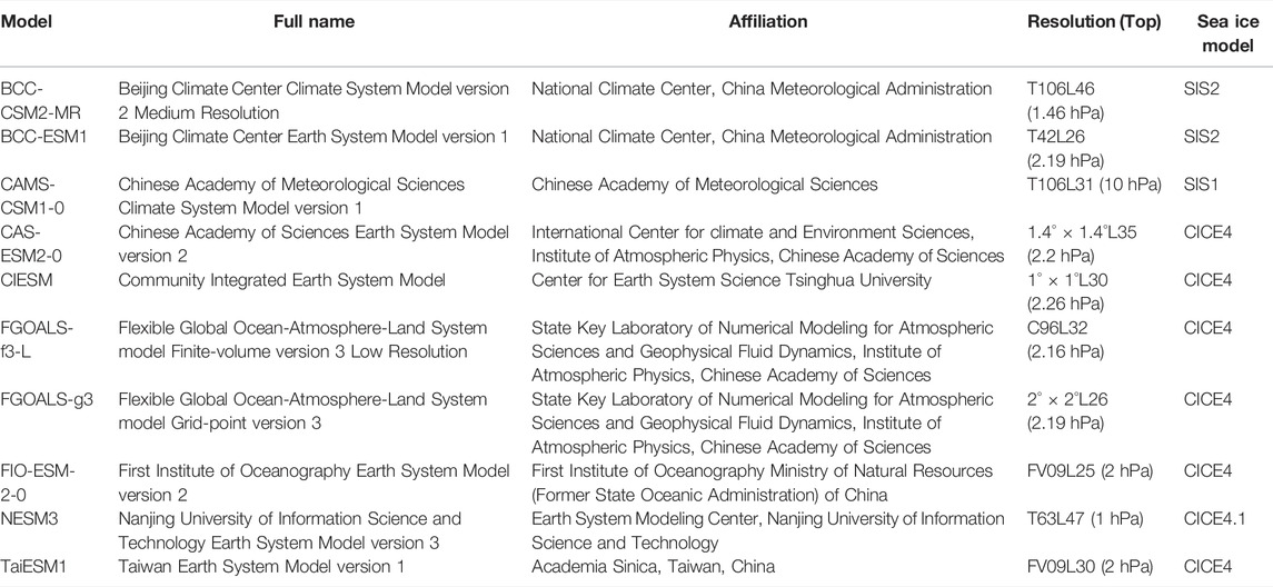
TABLE 1. Ten Chinese CMIP6 models tested in this study. The historical run is commonly available for the ten models.

Methods

To construct a possible physical relationship between the Arctic sea ice cover and China rainfall in early summer, the singular value decomposition (SVD) tool (Wallace et al., 1992) is applied in this study. The main purpose of the SVD tool is to find a linear combination for two sets of variables. This linear combination should meet the requirement with the largest covariance. The covariance maximization is calculated with orthogonality constraints on the coefficients of the linear combinations. To obtain the Arctic sea ice–China rainfall combination modes, the calculation is based on a SVD of the covariance matrix between observed sea ice and rainfall. The covariance matrix is obtained at grid points of the focused regions from two original geophysical fields (i.e., sea ice cover in Arctic and rainfall across China). Furthermore, the lead/lag regression is employed to obtain the maximum lead time of China rainfall by the state of Arctic sea ice.

Several indices are adopted in our study for estimating the linkage between Barents–Kara sea ice cover and eastern China rainfall. The Barents–Kara sea ice index refers to the area-averaged sea ice in the region across 65–85°N, 20–90°E. Two subregions have evident linkages with the Barents–Kara sea ice cover, one over 28–36°N, 110–122°E, and the other over 22–28°N, 105–122°E. The rainfall timeseries area-averaged over the two subregions are focused.

Mean State and Variability of the Arctic Sea Ice Cover in Early Winter

Figure 1 shows the climatology and variability of the Arctic sea ice concentration in November and December from 1979 to 2020. Most of the Arctic Ocean is covered by full sea ice except that the boundaries of the Arctic Ocean, continents and islands are not fully covered. It is also shown that most parts of North Pacific and North Atlantic Oceans are nearly free from sea ice (Figure 1A). Regions with full sea ice and regions free from sea ice concentration show little interannual variability, and the transition regions from full sea ice to open oceans and seas usually have relatively large variability in November and December (Figure 1B). The sea ice variability is largest in Barents–Kara Seas, standing out from other transition regions. The Barents–Kara Seas (65–85°N, 20–90°E) are a key region in this study, marked by a sector box in Figure 1.

FIGURE 1

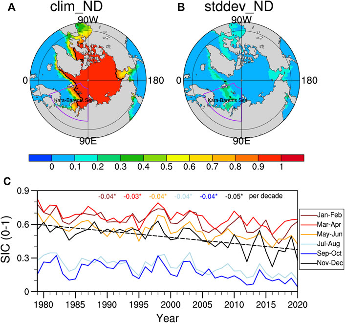
FIGURE 1. (A,B) Climatology and variability of the Arctic sea ice cover in November and December from 1979 to 2020. The sector box marks Barents–Kara Seas where the variability is relatively large (65–85°N, 20–90°E). (C) Time series (colored solid curves) of the sea ice cover in Barents–Kara Seas for every 2 months. The trend of the sea ice cover is also printed, and the black lines especially mark the trend in November–December. An asterisk is added if the trend is significant at the 95% confidence level.

Figure 1C presents the time series of the bimonthly averages of sea ice concentration in the Barents–Kara Seas. It is shown that the sea ice concentration in November–December shows a significant decreasing trend from 1979 to 2020. This significant decreasing trend is seen in other bimonthly means, and the November–December trend is the largest (−0.05 per decade). It can be concluded that in the Barents–Kara Seas, sea ice in November and December decreased the most from 1979 to 2020 out of the 12 months. Onarheim et al. (2018) also showed that in late autumn and early winter the sea ice variability is particularly pronounced in the Barents–Kara Seas.

Possible Impact of the Arctic Sea Ice Cover on June Rainfall in Eastern China

Singular Value Decomposition Analysis

To study the possible relationship between the sea ice in Barents–Kara Seas in November–December and June precipitation in China mainland (5–54°N, 72–136°E), we use the SVD tool to extract their combination modes. The three leading SVD modes for Arctic sea ice and China rainfall are shown in Figure 2. The first SVD mode explains 47% of the total covariance. The first SVD mode (SVD1) corresponds to a uniform variability of sea ice concentration in Kara and Barents Seas (Figure 2A). The second SVD mode (SVD2) shows a more local variability centered in Barents Sea, which only explains 14% of the total covariance (Figure 2B). In contrast, the third SVD (SVD3) contributes even much less to the total covariance (∼7%) with the maximum center in Kara Sea (Figure 2C).

FIGURE 2

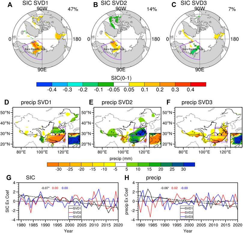
FIGURE 2. The singular value decomposition (SVD) of the Arctic sea ice cover in November–December and the June precipitation in China mainland (5–54°N, 72–136°E). (A–C) Left vectors reconstructed by regressing the Arctic sea ice cover against the standardized expansion coefficient of the left homogeneous field. The percent covariance explained by the SVD modes is printed on the top right for each plot. (D–F) Right vectors reconstructed by regressing the June rainfall anomalies against the standardized expansion coefficient of the right homogeneous field. The purple boxes show the relatively large rainfall variability centers (28–36°N, 110–122°E and 22–28°N, 105–122°E). (G,H) Standardized expansion coefficients of the left and right homogeneous fields. The trend for each expansion coefficient is also printed with the same color as for the curve. An asterisk is added if the trend is significant at the 95% confidence level.

Different rainfall response patterns in June form following the three different sea ice forcings (Figures 2D–F). In response to a uniform sea ice forcing in Barents–Kara Seas, a dipole rainfall pattern appears in June. This rainfall pattern corresponds to out-of-phase variations of rainfall in Yangtze–Huai Rivers Valley (28–36°N, 110–122°E) and South China (22–28°N, 105–122°E). Namely, the Barents–Kara sea ice increase (loss) in early winter excites anomalous more (less) June rainfall in Yangtze–Huai Rivers Valley and less (more) rainfall in South China. The individual Kara or Barents sea ice forcing usually corresponds to a uniform rainfall anomaly pattern in the eastern part of China, as shown in the SVD2 and SVD3 rainfall modes.

The standardized expansion coefficients of the left field (i.e., sea ice) and the right field (i.e., rainfall) are shown in Figures 2G,H. It is shown that the sea ice over Barents and Kara Seas has a significant decreasing trend from 1979 to 2020 (∼0.07), which might be due to the global warming (Long and Perrie, 2017). In contrast, no evident trend (∼0) in the second and third SVD modes is found. Consistent with the decreasing trend in the first Arctic sea ice mode, a significant trend is also found for the first rainfall pattern in eastern China (Figure 2H). The first mode exhibits a much larger trend (∼−0.06) than the other two SVD models. Combining the rainfall pattern and the coefficients, this trend denotes wetting of South China and/or drying of Yangtze–Huai Rivers Valley, which might be forced by the gradual loss of sea ice in the Barents–Kara Seas.

Linkage Between Arctic Sea Ice and June Rainfall in Eastern China

As seen from the SVD analysis, the uniform sea ice variability in the Barents–Kara Seas explained much more of the covariance than other modes, so this study focuses on the corresponding rainfall pattern. In the first rainfall mode, two variability centers are noticed, one across Yangtze–Huai Rivers Valley (28–36°N, 110–122°E) and the other across South China (22–28°N, 105–122°E). To further test the possible interannual and long-term change in the two regions, their area-averaged rainfall in June is shown in Figure 3 from three datasets. Consistent with the SVD1 expansion coefficient, a trend is noticed for rainfall especially in South China. Specifically, rainfall across Yangtze–Huai Rivers Valley presents an insignificant trend (Figure 3A), whereas the increasing trend in South China rainfall is evident in all of the three datasets (Figure 3B). Consistent conclusions based on the SVD analysis and Figure 3 might suggest a robust result.

FIGURE 3

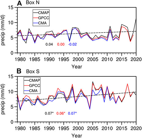
FIGURE 3. Time series of the June rainfall during 1979–2020 from three precipitation observations (CMAP, GCPP, and CMA station observations). The area-weighted mean rainfall over (A) the north box and (B) the south box in Figures 2D–F is focused. The trend in each dataset is printed, and an asterisk is added if the trend (units; mm/d/yr) is significant at the 95% confidence level.

To further test the relationship between local rainfall and Barents–Kara sea ice for Yangtze–Huai Rivers Valley and South China, scatterplots of sea ice versus rainfall are shown in Figure 4 based on three precipitation data (CMAP, GPCC, and CMA). In the interannual timescale, a positive correlation is found for Barents–Kara sea ice concentration and June rainfall in Yangtze–Huai Rivers Valley (Figures 4A,C,E), consistent with the SVD analysis. Correlation between the sea ice and rainfall is largest in the CMA observations than in another two datasets (R = 0.22, 0.37, 0.55) with the highest confidence level ($\alpha$ = 0.17, 0.02, 0.00). This small divergence of the correlation and its significance level might be caused by the different resolutions and timespans available. Similarly, a negative correlation is established for Barents–Kara sea ice concentration and June rainfall in South China (Figures 4B,D,F), consistently among three precipitation datasets. The correlation and its significance level are largest in CMAP than in another two datasets.

FIGURE 4

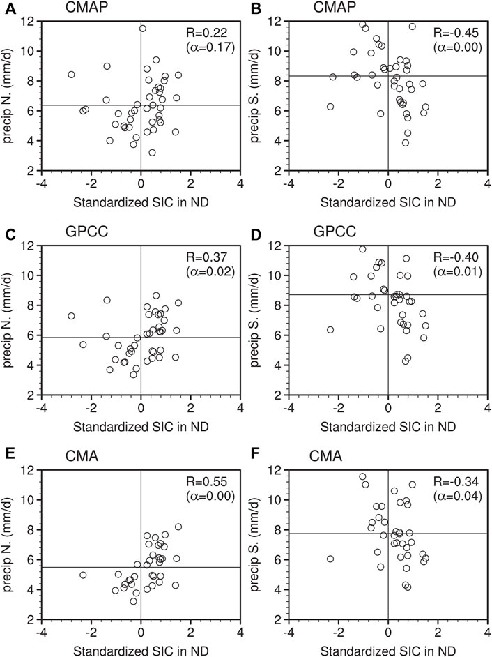
FIGURE 4. Scatterplots of the standardized November–December mean sea ice concentration in Barents–Kara Seas versus the precipitations in the north (A), (C), (E) and south (B), (D), (F) box in Figures 2D–F for three rainfall datasets. The correlation between the sea ice and precipitation and its significance level are also printed on the top right for each plot.

The evolution of regressed monthly rainfall anomalies against the November–December sea ice in the Barents–Kara Seas is shown in Figure 5. We will test if the rainfall response to Arctic sea ice forcing is maximized in June. East Asia is strongly controlled by the monsoon, and rainfall response is generally weak in dry season months. The concurrent regression pattern shows that the Barents–Kara sea ice increase (loss) usually induces anomalously less (more) rainfall in eastern China (Figures 5A,B), which is caused by the circulation change related to the thermal forcing associated with the sea ice change (Shen et al., 2019). No evident dry or wet pattern is seen in later months, which might be due to the prevailing of the climatological westerlies and unfavorable moisture conditions in those months (Figures 5C–F). As the climatological seasonal rainbelt forms and moves northward since May, the anomaly pattern more easily forms (Figure 5G). The maximum rain response in China to preceding Barents–Kara sea ice forcing appears in June (Figure 5H) and weakens soon (not shown).

FIGURE 5

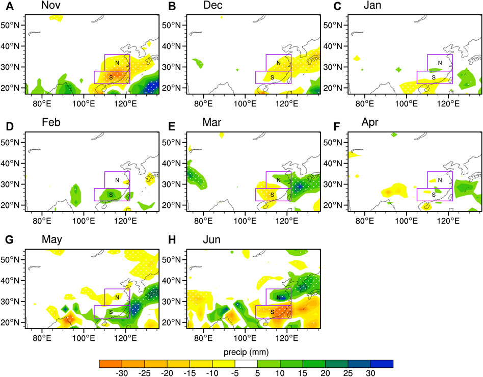
FIGURE 5. Evolution of regressed CMAP rainfall anomalies (units: mm) from (A–H) November to June against the standardized November–December mean Arctic sea ice concentration in Barents–Kara Seas. The boxes marked are the same as in Figures 2D–F. The dotted regions show the regression at the 95% confidence level.

To verify the robustness of the rainfall response pattern and its independence of the choice of the rainfall datasets, the regressed June rainfall pattern is shown in Figure 6 for CMAP, GPCC, and CMA observations. The dipole rainfall pattern is consistently revealed by the three datasets, which further verify the SVD1 pattern associated with a uniform sea ice forcing across Kara and Barents Seas. Following a sea ice increase in Barents–Kara Seas, Yangtze–Huai Rivers Valley tends to get wet, but South China gets dry in early summer. The anomaly magnitude in the dipole centers is stronger in CMA observations (Figure 6C) than in CMAP and GPCC (Figures 6A,B), but the general pattern is highly similar.

FIGURE 6

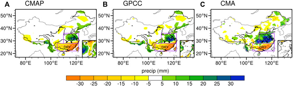
FIGURE 6. Regression of June rainfall anomalies (units: mm) against the standardized November–December mean Arctic sea ice concentration in Barents–Kara Seas in the preceding early winter. The three rainfall datasets are shown, including (A) CAMP, (B) GPCC, and (C) CMA. The boxes marked are the same as in Figures 2D–F. The dotted regions show the regression at the 95% confidence level.

How Does the Arctic Sea Ice in Early Winter Affect the Early Summer Rainfall?

The possible impact of spring–summer Arctic sea ice anomalies on the Northern Hemisphere atmospheric circulation has been explored in recent studies (Zhang et al., 2018b; Wu and Li, 2021). Zhang et al. (2018b) found that the spring–summer Arctic sea ice is positively correlated with the Ural blocking frequency in summer due to a midlatitude wave train spanning across Eurasia. Since the relationship between Barents–Kara sea ice in early winter and China rainfall in June has been established, the mechanism whereby this pathway forms is still not understood. Next, we will explain the possible impact of Arctic sea ice variation on rainfall in eastern China. One possible reason for the long-lasting lagged impact of sea ice is due to its long memory. Figure 7 shows the lead/lag regression of sea ice anomalies against the Barents–Kara sea ice index. Following significant sea ice growth (or loss) in the focused region (65–85°N, 20–90°E) in November and December (Figure 7A), this uniform pattern is nearly unchanged until January and February (Figure 7B). The coverage and area of significant sea ice concentration anomalies shrink in March and April (Figure 7C), but the anomaly pattern still remains. Afterwards, the sea ice pattern covered by significant anomalies persists until May and June (Figure 7D). The long-lasting sea ice anomaly forcing favors a persisting lagged impact on the circulation and rainfall.

FIGURE 7

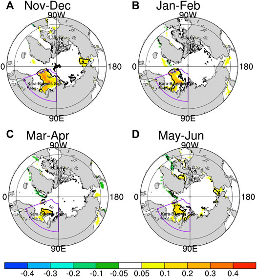
FIGURE 7. Evolution of regressed Arctic sea ice concentration anomalies (units: dimensionless) from (A–D) November–December to May–June against the standardized November–December mean Arctic sea ice concentration in Barents–Kara Seas as marked in the purple sector. The black contours show the regression at the 95% confidence level.

Next, the evolution of regressed atmospheric circulation from the stratosphere to the troposphere against the November–December Barents–Kara sea ice index is shown in Figure 8. Following the Barents–Kara sea ice change in November–December, instant significant circulation anomalies are observed from the stratosphere to the troposphere. In the sea ice growth years, negative height anomalies form over the Arctic, while positive anomalies appear in midlatitudes during November–December (Figure 8A). This pattern resembles the positive phase of the northern annular mode (NAM) projected from a strong polar vortex. The stratospheric polar vortex continues to strengthen, and therefore, this positive NAM-like pattern enhances in the following January and February (Figure 8B). In March and April, this pattern begins to reverse and the NAM pattern seems to weaken. A wavenumber-2-like pattern develops in March and April (Figure 8C). This might indicate that the suppressed waves in early and midwinter associated with the strong polar vortex tend to be activated in spring to weaken the polar vortex. This out-of-phase change of the polar vortex in winter and spring was noticed by Hu et al. (2014). During May and June, negative height anomalies develop in midlatitudes, and weak positive height anomalies form over the Arctic Ocean, which can be projected onto the negative NAM pattern (Figure 8D). Previous studies have reported that the stratospheric response to the Arctic sea ice loss is similar but with the sign reversed (Kim et al., 2014; Cohen et al., 2021; Xu et al., 2021).

FIGURE 8

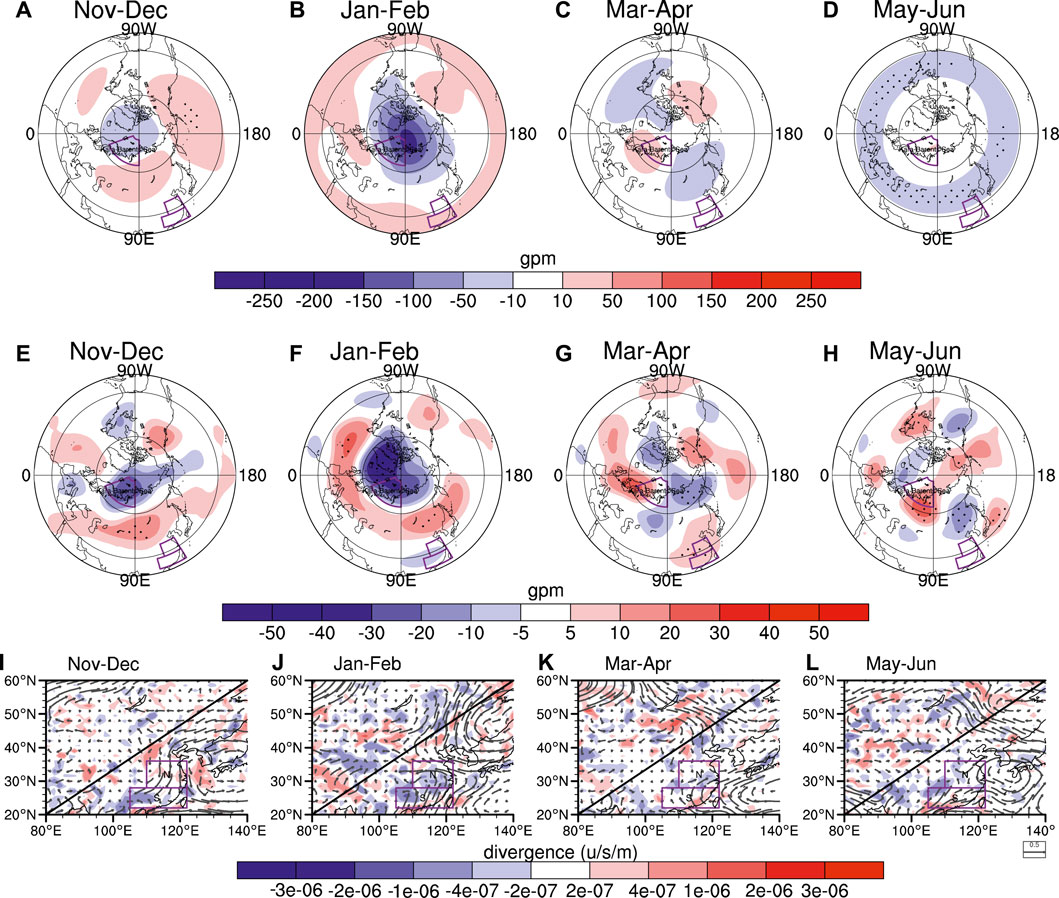
FIGURE 8. (A–D) Evolution of regressed (top row) geopotential height anomalies at 10 hPa (units: gpm) from November–December to May–June against the standardized November–December mean Arctic sea ice concentration in Barents–Kara Seas. The dotted regions show the regression at the 95% confidence level. (E–H) as in (A–D) but for geopotential height anomalies at 200 hPa. (I–L) as in (A–D) but for horizonal wind anomalies and divergence anomalies at 850 hPa.

Following changes in the stratospheric circulation, the evolution of the tropospheric anomaly pattern is also noted. Similar to the stratospheric anomaly pattern, negative height anomalies are also seen over the Arctic at 200 hPa from November to February, whereas in midlatitude annular positive height anomalies form (Figures 8E,F). Namely, positive NAM anomaly pattern is also observed from November to February at 200 hPa. As the sea ice anomaly forcing shrinks in March and later months, negative height anomalies over the Arctic also shrink and move to northeastern Asia, whereas positive height anomalies in midlatitudes shrink and move to eastern China (Figure 8G). The circulation anomaly pattern at 200 hPa in March and April is a wave train like teleconnection spanning from Barents–Kara Seas to China. Following the sea ice increase in Barents–Kara Seas, a positive height anomaly lobe appears locally in spring; a negative height anomaly lobe forms over Western Asia; and a positive height anomaly lobe appears in South China. This wave pattern shifts further eastwards in May and June (Figure 8H). Specifically, a positive height anomaly lobe appears over Siberia; a negative height anomaly lobe forms to the east of Baikal; a positive height anomaly lobe appears over Japan.

Lead/lag regression of the circulation anomalies at 850 hPa against the Barents–Kara sea ice index in November–December is shown in Figures 8I–L. Consistent with the development of positive height anomalies in midlatitudes (centered in Central Asia), northerly anomalies appear in eastern China (Figures 8E,I). Following sea ice increase, anomalous northerlies control most of eastern China, consistent with the dry conditions in November and December. As the positive height anomaly center in Siberia moves further eastward to northeastern Asia, a negative height anomaly center forms in South China in January and February at 200 hPa, which is also seen at 850 hPa, denoted by the anomalous cyclonic circulation in South China (Figures 8F,J). The annular pattern gradually weakens, replaced by a wave train like pattern in March and April, and an anomalous anticyclone develops in eastern China at 200 hPa, which is biased to East China Sea at 850 hPa (Figures 8G,K). Anomalous southerly winds developed in most of South China, although the rainfall anomalies are still not evident in March and April. As the wave train like pattern shifts further eastward in May and June, it is also observed that a negative height anomaly center controls northeastern China at 200 hPa, which shifts to the ocean at 850 hPa (Figures 8H,L). It is observed that anomalous northerlies in the west of the cyclone over the East China Sea converge with the southwesterlies in Yangtze–Huai Rivers Valley at 850 hPa, well explaining the local wet condition in June associated with the sea ice increase in preceding early winter. Strong southwesterly anomalies in South China correspond to the local dry conditions.

The circulation response to the Arctic sea ice forcing varies with the season possibly due to the change of the mean state. In addition, we also find that the stratospheric response tends to be out-of-phase in winter and in spring. In other words, a dormant stratospheric polar vortex in winter tends to be disturbed in spring, while a perturbed stratospheric polar vortex in winter tends to be strong in early spring (e.g., Hu et al., 2014).

We will try to understand the possible impact of sea ice from the coupling between stratosphere–troposphere–cryosphere. The stratospheric polar vortex plays an important role in the stratospheric-tropospheric dynamic coupling (Kodera et al., 1991; Baldwin and Dunkerton, 2001). The lead/lag regression of the circumpolar wind and polar cap temperature against the November–December sea ice in Barents–Kara Seas is shown in Figure 9. Following an increase in sea ice, the stratospheric polar vortex strengthens in November–February, corresponding to the enhancement of the meridional gradient of heights in the circumpolar region. In other words, the circumpolar westerly winds accelerate, denoted by positive zonal wind anomalies from November to February throughout the stratosphere and troposphere (Figure 9A). The westerly response gets maximized in January and shows a downward propagation. This strengthening of the polar vortex is followed by the weakening of the vortex, denoted by the easterly anomalies in the circumpolar region. This is consistent with the development of the negative NAM in March and April. However, the annular like response gradually diminishes in May and June when the stratosphere–troposphere coupling is weak, but the wave-like anomaly pattern is most evident in the troposphere.

FIGURE 9

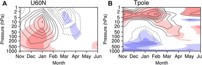
FIGURE 9. Pressure-temporal evolutions of (A) regressed circumpolar zonal wind anomalies at 60°N (units: m/s) and (B) regressed polar cap temperature anomalies (units: °C) averaged over 60–90°N against the standardized November–December mean Arctic sea ice concentration in Barents–Kara Seas, representing the stratosphere–troposphere–cryosphere coupling. The dark and light shadings mark the regression at the 90% and 95% confidence levels, respectively.

In cold season months, the circulation response is more annular, while in early warm season months, the anomaly pattern highly resembles a wave train. The annular response in cold season months can also be seen from the evolution of the polar cap temperature, as another representation of the polar vortex strength (Figure 9B). In the troposphere and lower stratosphere, cold anomalies develop from November to February, consistent with the strong and cold state of the polar vortex. In the upper stratosphere, warm anomalies form and propagate downward to lower levels after March. Warm anomalies replace cold anomalies in March and later months, consistent with the reversal of the NAM phase. In May and June, temperature anomalies largely diminish, further verifying the weakening of the annular mode-like anomaly pattern in the warm season months associated with the sea ice forcing in Barents–Kara Seas.

Can CMIP6 Models Reproduce the Arctic Sea Ice–China Rainfall Relationship?

The lagged impact of the Barents–Kara sea ice in November–December on China rainfall in June is observed, but it is still unknown if the state-of-the-art models can simulate the sea ice–rainfall relationship. Next, the performance of the CMIP6 models is evaluated for this relationship. Lead/lag regression of China rainfall in June against the sea ice index in November–December is shown in Figure 10 for 10 Chinese CMIP6 models. In general, very few models can accurately produce the observed relationship between sea ice and China rainfall. It is observed that more rainfall in Yangtze–Huai Rivers Valley follows sea ice growth, whereas less rainfall appears in South China (Figure 10K). In contrast, only CAMS-CSM1-0 and FIO-ESM-2-0 can limitedly (but not accurately) produce the rainfall dipole pattern, wet in the north and dry in the south (Figures 10C,H). The simulated rainfall pattern by these two models is somewhat different from the observations.

FIGURE 10

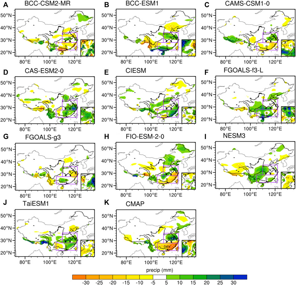
FIGURE 10. Underrepresentation of CMIP6 models in producing the linkage between the November–December mean Arctic sea ice in Barents–Kara Seas and the June rainfall in China mainland. (A–J) Regression of June rainfall anomalies (units: mm) against the standardized November–December mean Arctic sea ice concentration in Barents–Kara Seas in the preceding early winter for 10 models from China. (K) Replicated from Figure 6A showing the regression for CMAP as a verification reference.

Other models tend to simulate a monopole rainfall pattern in eastern China. For example, a dry pattern is simulated across most of eastern China following sea ice growth by BCC-CSM2-MR (Figure 10A), while a uniform wet pattern is simulated in CAS-ESM2-0, CIESM, FGOALS-f3-L, and TaiESM1 (Figures 10D–G). Other models only simulated rather local illusive rainfall response (BCC-ESM1, FGOALS-g3, and NESM3). It is still a great challenge for most models to simulate the pathways for Arctic sea ice growth or loss. The simulated rainfall response pattern diverges among CMIP6 models.

The underrepresentation of the sea ice–rainfall relationship is a deficiency for CMIP6 models, which might contribute to the uncertainty of the climate projection in the future. Existing studies have shown that coupled models still have great uncertainty in simulating the amplitude and changing trend of sea ice (Stroeve et al., 2007; Kay et al., 2011), which might limit the reproduction of the sea ice–rainfall relation.

Conclusion and Discussion

Conclusion

Using the sea ice concentration dataset provided by the Met Office Hadley Centre during 1979–2020 when remote sensing observations have been available, the long-term mean and variability of the Arctic sea ice are tested. We find that sea ice concentration is nearly full in most of the Arctic, and sea ice variability is usually large in regions with some but not full sea ice concentration. Barents–Kara Seas are an interconnected region with relatively large sea ice variability. From the perspective of the annual cycle for the long-term mean, sea ice in this region gradually grows from autumn to spring and melts from spring to autumn. Sea ice concentration gets maximized in April and gets minimized in September. The long-term melting trend for Barents–Kara sea ice is identified for all seasons, and this trend is largest in November and December when the interannual variability is also large.

To reveal the possible lead/lag linkage between sea ice variability in Barents–Kara Seas, the SVD tool is used to extract the leading coupled mode patterns. It is found that the first SVD mode explains nearly half of the total variance, which is characterized by the uniform sea ice change in Barents–Kara Seas, consistent with the interannual variability pattern. Following a uniform change of the sea ice in Barents–Kara Seas, a dipole rainfall pattern across eastern China appears. Sea ice growth corresponds to more rainfall in Yangtze–Huai Rivers Valley and less rainfall in South China. With the linear assumption, sea ice loss in Barents–Kara Seas should be followed by an opposite rainfall pattern. In contrast, the second and third SVD modes explain the variance much less than the first one, corresponding to a monopole rainfall anomaly pattern. Consistent with the decreasing trend in Barents–Kara sea ice extracted from the leading SVD, an increasing trend in South China rainfall is also observed.

The long-lasting lagged impact of sea ice on rainfall is likely associated with the long memory of the sea ice and the circulation change forced by the sea ice variations. Diagnostic analysis shows that the anomaly pattern of the sea ice in Barents–Kara Seas can persist from November to the following early summer, although the magnitude gradually diminishes. The atmospheric response to the Barents–Kara sea ice forcing varies with the season. In winter and spring when the stratosphere–troposphere coupling is strong, the atmospheric response resembles an annular mode pattern from the stratosphere to the troposphere. The stratospheric response in winter tends to be out of phase with that in spring: sea ice growth (loss) leads to a positive (negative) NAM response in winter but negative (positive) NAM response in spring. Namely, the stratospheric polar vortex intensifies soon following the sea ice growth, and a dormant stratospheric circulation in winter is usually followed by more perturbed period in spring due to the internal adjustment of the atmosphere. The stratospheric signal shows a downward propagation in winter and spring, and the annular mode like response is also observed in the troposphere. A uniform dry pattern is observed across eastern China in winter when the Barents–Kara sea ice concentration increases. However, the NAM-like response does not persist until early summer.

In May and June, the annular mode response gradually weakens and is replaced by a wave train pattern. Associated with Barents–Kara sea ice growth, an anomalous cyclone over Yellow Sea and an anomalous anticyclone over East China Sea are observed in May and June. Anomalous northeasterly and southwesterly winds converge over Yangtze–Huai Rivers Valley, so a dry South China and wet Yangtze–Huai Rivers Valley pattern finally forms in June.

The observed sea ice–eastern China rainfall linkage is limitedly simulated in CMIP6 models. Only CAMS-CSM1-0 and FIO-ESM-2-0 reproduce the dipole rainfall pattern associated with Barents–Kara sea ice growth (or loss). However, the rainfall response amplitude is much smaller than in the observations. Other models illusively simulate a monopole rainfall pattern or insignificant signals in the rainfall. Therefore, it is still a big challenge for most models to capture the linkage between sea ice and China rainfall, and further improvement is still required.

Discussion

The varying response in the extratropics with the season is related to the mean state of the circulation. In winter and early spring, planetary waves can propagate upward into the stratosphere and the stratosphere–troposphere coupling is strong (Reichler et al., 2005; Shaw and Perlwitz, 2013). In this way, the NAM response in the stratosphere to sea ice variability can propagate downward to modulate the tropospheric circulation. However, in warm seasons, planetary waves cannot propagate upward into the stratosphere due to prevailing of circumpolar easterlies in summer. The tropospheric response to sea ice in early summer resembles a wave train, spanning from Barents–Kara Seas to northwestern Pacific.

Due to the feedback of snow and sea ice albedo, the Arctic is particularly sensitive to global climate changes (Holland and Bitz, 2003). The reduction of sea ice in the Arctic region further leads to an increase in temperature, which then feeds back to the sea ice loss again. Therefore, the warming amplitude in the Arctic is usually much larger than in other latitudes of the globe (Alexander et al., 2004; Honda et al., 2009). CMIP6 models still show large biases in simulation of the Arctic sea ice and climate (Davy and Outten, 2020; Long et al., 2021; Shen et al., 2021; Watts et al., 2021), which might contribute to the underrepresentation of the sea ice–China rainfall linkage in most models. Therefore, the state of the Arctic sea ice can modulate the atmospheric thermodynamic and dynamic processes, and any bias in the sea ice might lead to an underestimation of the climate response regionally and globally.

Our study has revealed the possible impact of sea ice change in Barents–Kara Seas on China rainfall. However, the change of Arctic sea ice is also affected by other factors (Heorton et al., 2014). The coverage of sea ice, the thickness of sea ice, and the speed of sea ice can affect but is also affected by the atmospheric conditions. Sensitivity experiments are still required to confirm the possible lagged impact of sea ice in Barents–Kara Seas on China rainfall in the future. Considering that the maximum coupling appears when Barents–Kara sea ice leads eastern China rainfall by nearly half a year, and that the sea ice has a long memory, the sea ice state is still a potential predictor for China rainfall prediction, left for future investigation.

Data Availability Statement

Publicly available datasets were analyzed in this study. This data can be found here: The authors thank the ECMWF for providing the ERA5 reanalysis (https://cds.climate.copernicus.eu). Arctic sea ice concentration data are freely available from UK Met office (https://www.metoffice.gov.uk/hadobs/hadisst/data/download.html). CMAP (https://psl.noaa.gov/data/gridded/data.cmap.html) and GPCC (https://psl.noaa.gov/data/gridded/data.gpcc.html) precipitation data are provided by the NOAA/OAR/ESRL PSL. China station precipitation data can only be obtained from CMA after the registration is authorized (http://data.cma.cn/).

Author Contributions

JR and HC led the conception and design of the manuscript. JR collected the data. HY analyzed the data and wrote the manuscript. All authors contributed to the development of ideas and manuscript revision and approved the submitted version.

Funding

This study was supported by the National Natural Science Foundation of China (Grant nos 42088101 and 42175069).

Conflict of Interest

The authors declare that the research was conducted in the absence of any commercial or financial relationships that could be construed as a potential conflict of interest.

Publisher’s Note

All claims expressed in this article are solely those of the authors and do not necessarily represent those of their affiliated organizations, or those of the publisher, the editors, and the reviewers. Any product that may be evaluated in this article, or claim that may be made by its manufacturer, is not guaranteed or endorsed by the publisher.

Acknowledgments

The authors acknowledge the National Natural Science Foundation of China for supporting this study. The authors also thank several agencies for providing their free multiple databases.

References

Alexander, M. A., Bhatt, U. S., Walsh, J. E., Timlin, M. S., Miller, J. S., and Scott, J. D. (2004). The Atmospheric Response to Realistic Arctic Sea Ice Anomalies in an AGCM during winter. J. Clim. 17 (5), 890–905. doi:10.1175/1520-0442(2004)017<0890:tartra>2.0.co;2

CrossRef Full Text | Google Scholar

Årthun, M., Eldevik, T., Smedsrud, L. H., Skagseth, Ø., and Ingvaldsen, R. B. (2012). Quantifying the Influence of Atlantic Heat on Barents Sea Ice Variability and Retreat. J. Clim. 25 (13), 4736–4743. doi:10.1175/JCLI-D-11-00466.1

CrossRef Full Text | Google Scholar

Baldwin, M. P., and Dunkerton, T. J. (2001). Stratospheric Harbingers of Anomalous Weather Regimes. Science 294 (5542), 581–584. doi:10.1126/science.1063315

PubMed Abstract | CrossRef Full Text | Google Scholar

Blackport, R., and Screen, J. A. (2020). Insignificant Effect of Arctic Amplification on the Amplitude of Midlatitude Atmospheric Waves. Sci. Adv. 6 (8), eaay2880. doi:10.1126/sciadv.aay2880

PubMed Abstract | CrossRef Full Text | Google Scholar

Blackport, R., Screen, J. A., van der Wiel, K., and Bintanja, R. (2019). Minimal Influence of Reduced Arctic Sea Ice on Coincident Cold winters in Mid-latitudes. Nat. Clim. Chang. 9 (9), 697–704. doi:10.1038/s41558-019-0551-4

CrossRef Full Text | Google Scholar

Cohen, J., Agel, L., Barlow, M., Garfinkel, C. I., and White, I. (2021). Linking Arctic Variability and Change with Extreme winter Weather in the United States. Science 373 (6559), 1116–1121. doi:10.1126/science.abi9167

PubMed Abstract | CrossRef Full Text | Google Scholar

Cohen, J., Zhang, X., Francis, J., Jung, T., Kwok, R., Overland, J., et al. (2020). Divergent Consensuses on Arctic Amplification Influence on Midlatitude Severe winter Weather. Nat. Clim. Chang. 10, 20–29. doi:10.1038/s41558-019-0662-y

CrossRef Full Text | Google Scholar

Comiso, J. C., Parkinson, C. L., Gersten, R., and Stock, L. (2008). Accelerated Decline in the Arctic Sea Ice Cover. Geophys. Res. Lett. 35 (1), 179–210. doi:10.1029/2007GL031972

CrossRef Full Text | Google Scholar

Cutty, J. A., Schramm, J. L., and Ebert, E. E. (1995). Sea Ice-Albedo Climate Feedback Mechanism. J. Clim. 8 (2), 240–247. doi:10.1175/1520-0442(1995)008<0240:SIACFM>2.0.CO;2

CrossRef Full Text | Google Scholar

Davy, R., and Outten, S. (2020). The Arctic Surface Climate in CMIP6: Status and Developments since CMIP5. J. Clim. 33 (18), 8047–8068. doi:10.1175/JCLI-D-19-0990.1

CrossRef Full Text | Google Scholar

Deser, C., and Teng, H. (2008). Evolution of Arctic Sea Ice Concentration Trends and the Role of Atmospheric Circulation Forcing, 1979-2007. Geophys. Res. Lett. 35 (2), L02504. doi:10.1029/2007gl032023

CrossRef Full Text | Google Scholar

Ding, S., Wu, B., and Chen, W. (2021). Dominant Characteristics of Early Autumn Arctic Sea Ice Variability and its Impact on winter Eurasian Climate. J. Clim. 34 (5), 1825–1846. doi:10.1175/jcli-d-19-0834.1

CrossRef Full Text | Google Scholar

Ding, S., and Wu, B. (2021). Linkage between Autumn Sea Ice Loss and Ensuing spring Eurasian Temperature. Clim. Dyn. 57 (9), 2793–2810. doi:10.1007/s00382-021-05839-0

CrossRef Full Text | Google Scholar

Francis, J. A., Chan, W. H., Leathers, D. J., Miller, J. R., and Veron, D. E. (2009). Winter Northern Hemisphere Weather Patterns Remember Summer Arctic Sea-Ice Extent. Geophys. Res. Lett. 36 (7), 157–136. doi:10.1029/2009gl037274

CrossRef Full Text | Google Scholar

Gastineau, G., García-Serrano, J., and Frankignoul, C. (2017). The Influence of Autumnal Eurasian Snow Cover on Climate and its Link with Arctic Sea Ice Cover. J. Clim. 30 (19), 7599–7619. doi:10.1175/JCLI-D-16-0623.1

CrossRef Full Text | Google Scholar

Guo, D., Gao, Y. Q., Bethke, I., Gong, D. Y., Johannessen, O. M., and Wang, H. J. (2014). Mechanism on How the spring Arctic Sea Ice Impacts the East Asian Summer Monsoon. Theor. Appl. Climatol. 115 (1-2), 107–119. doi:10.1007/s00704-013-0872-6

CrossRef Full Text | Google Scholar

Heorton, H. D. B. S., Feltham, D. L., and Hunt, J. C. R. (2014). The Response of the Sea Ice Edge to Atmospheric and Oceanic Jet Formation. J. Phys. Oceanogr. 44 (9), 2292–2316. doi:10.1175/jpo-d-13-0184.1

CrossRef Full Text | Google Scholar

Hersbach, H., Bell, B., Berrisford, P., Hirahara, S., Horányi, A., Muñoz‐Sabater, J., et al. (2020). The ERA5 Global Reanalysis. Q.J.R. Meteorol. Soc. 146 (730), 1999–2049. doi:10.1002/qj.3803

CrossRef Full Text | Google Scholar

Holland, M. M., and Bitz, C. M. (2003). Polar Amplification of Climate Change in Coupled Models. Clim. Dyn. 21 (3-4), 221–232. doi:10.1007/s00382-003-0332-6

CrossRef Full Text | Google Scholar

Honda, M. J., Inoue, J., and Yamane, S. (2009). Influence of Low Arctic Sea‐ice Minima on Anomalously Cold Eurasian winters. Geophys. Res. Lett. 36 (8), L08707. doi:10.1029/2008GL037079

CrossRef Full Text | Google Scholar

Hu, J., Ren, R., and Xu, H. (2014). Occurrence of winter Stratospheric Sudden Warming Events and the Seasonal Timing of spring Stratospheric Final Warming. J. Atmos. Sci. 71 (7), 2319–2334. doi:10.1175/jas-d-13-0349.1

CrossRef Full Text | Google Scholar

Kay, J. E., Holland, M. M., and Jahn, A. (2011). Inter-annual to Multi-Decadal Arctic Sea Ice Extent Trends in a Warming World. Geophys. Res. Lett. 38 (15), L15708. doi:10.1029/2011gl048008

CrossRef Full Text | Google Scholar

Kelleher, M. E., Ayarzagüena, B., and Screen, J. A. (2020). Interseasonal Connections between the Timing of the Stratospheric Final Warming and Arctic Sea Ice. J. Clim. 33 (8), 3079–3092. doi:10.1175/jcli-d-19-0064.1

CrossRef Full Text | Google Scholar

Kim, B.-M., Son, S.-W., Min, S.-K., Jeong, J.-H., Kim, S.-J., Zhang, X., et al. (2014). Weakening of the Stratospheric Polar Vortex by Arctic Sea-Ice Loss. Nat. Commun. 5, 4646. doi:10.1038/ncomms5646

PubMed Abstract | CrossRef Full Text | Google Scholar

Kodera, K., Chiba, M., Yamazaki, K., and Shibata, K. (1991). A Possible Influence of the Polar Night Stratospheric Jet on the Subtropical Tropospheric Jet. J. Meteorol. Soc. Jpn. 69 (6), 715–721. doi:10.2151/jmsj1965.69.6_715

CrossRef Full Text | Google Scholar

Li, H., Chen, H., Wang, H., Sun, J., and Ma, J. (2018). Can Barents Sea Ice Decline in spring Enhance Summer Hot Drought Events over Northeastern China? J. Clim. 31 (12), 4705–4725. doi:10.1175/jcli-d-17-0429.1

CrossRef Full Text | Google Scholar

Li, Y., and Leung, L. R. (2013). Potential Impacts of the Arctic on Interannual and Interdecadal Summer Precipitation over China. J. Clim. 26 (3), 899–917. doi:10.1175/JCLI-D-12-00075.1

CrossRef Full Text | Google Scholar

Lin, Z.-D., and Li, F. (2018). Impact of Interannual Variations of spring Sea Ice in the Barents Sea on East Asian Rainfall in June. Atmos. Oceanic Sci. Lett. 11 (3), 275–281. doi:10.1080/16742834.2018.1454249

CrossRef Full Text | Google Scholar

Lindsay, R. W., Zhang, J., Schweiger, A., Steele, M., and Stern, H. (2009). Arctic Sea Ice Retreat in 2007 Follows Thinning Trend. J. Clim. 22 (13), 165–176. doi:10.1029/96GL01426

CrossRef Full Text | Google Scholar

Liu, J. P., Curry, J. A., Wang, H., Song, M., and Horton, R. (2012). Impact of Declining Arctic Sea Ice on winter Snowfall. Proc. Natl. Acad. Sci. USA 109 (11), 4074–4079. doi:10.1073/pnas.1114910109

PubMed Abstract | CrossRef Full Text | Google Scholar

Liu, Y., Zhu, Y., Wang, H., Gao, Y., Sun, J., Wang, T., et al. (2019). Role of Autumn Arctic Sea Ice in the Subsequent Summer Precipitation Variability over East Asia. Int. J. Climatol 40, 706–722. doi:10.1002/joc.6232

CrossRef Full Text | Google Scholar

Long, M., Zhang, L., Hu, S., and Qian, S. (2021). Multi-aspect Assessment of CMIP6 Models for Arctic Sea Ice Simulation. J. Clim. 34 (4), 1515–1529. doi:10.1175/jcli-d-20-0522.1

CrossRef Full Text | Google Scholar

Long, Z., and Perrie, W. (2017). Changes in Ocean Temperature in the Barents Sea in the Twenty-First century. J. Clim. 30 (15), 5901–5921. doi:10.1175/jcli-d-16-0415.1

CrossRef Full Text | Google Scholar

Lukovich, J. V., and Barber, D. G. (2006). Atmospheric Controls on Sea Ice Motion in the Southern Beaufort Sea. J. Geophys. Res. 111, D18103. doi:10.1029/2005jd006408

CrossRef Full Text | Google Scholar

Luo, D., Chen, X., Dai, A., and Simmonds, I. (2018). Changes in Atmospheric Blocking Circulations Linked with winter Arctic Warming: a New Perspective. J. Clim. 31 (18), 7661–7678. doi:10.1175/jcli-d-18-0040.1

CrossRef Full Text | Google Scholar

Luo, D., Chen, X., Overland, J., Simmonds, I., Wu, Y., and Zhang, P. (2019). Weakened Potential Vorticity Barrier Linked to Recent winter Arctic Sea Ice Loss and Midlatitude Cold Extremes. J. Clim. 32 (14), 4235–4261. doi:10.1175/jcli-d-18-0449.1

CrossRef Full Text | Google Scholar

Mori, M., Watanabe, M., Shiogama, H., Inoue, J., and Kimoto, M. (2014). Robust Arctic Sea-Ice Influence on the Frequent Eurasian Cold winters in Past Decades. Nat. Geosci 7 (12), 869–873. doi:10.1038/ngeo2277

CrossRef Full Text | Google Scholar

Newson, R. L. (1973). Response of a General Circulation Model of the Atmosphere to Removal of the Arctic Ice-Cap. Nature 241, 39–40. doi:10.1038/241039b0

CrossRef Full Text | Google Scholar

Onarheim, I. H., Eldevik, T., Smedsrud, L. H., and Stroeve, J. C. (2018). Seasonal and Regional Manifestation of Arctic Sea Ice Loss. J. Clim. 31 (12), 4917–4932. doi:10.1175/jcli-d-17-0427.1

CrossRef Full Text | Google Scholar

Outten, S. D., and Esau, I. (2012). A Link between Arctic Sea Ice and Recent Cooling Trends over Eurasia. Climatic Change 110 (3-4), 1069–1075. doi:10.1007/s10584-011-0334-z

CrossRef Full Text | Google Scholar

Parkinson, C. L., and Comiso, J. C. (2013). On the 2012 Record Low Arctic Sea Ice Cover: Combined Impact of Preconditioning and an August Storm. Geophys. Res. Lett. 40 (7), 1356–1361. doi:10.1002/grl.50349

CrossRef Full Text | Google Scholar

Petoukhov, V., and Semenov, V. A. (2010). A Link between Reduced Barents-Kara Sea Ice and Cold winter Extremes over Northern Continents. J. Geophys. Res. 115, D21111. doi:10.1029/2009JD013568

CrossRef Full Text | Google Scholar

Raymo, M. E., Rind, D., and Ruddiman, W. F. (1990). Climatic Effects of Reduced Arctic Sea Ice Limits in the GISS II General Circulation Model. Paleoceanography 5 (3), 367–382. doi:10.1029/pa005i003p00367

CrossRef Full Text | Google Scholar

Rayner, N. A., Parker, D. E., Horton, E. B., Folland, C. K., Alexander, L. V., Rowell, D. P., et al. (2003). Global Analyses of Sea Surface Temperature, Sea Ice, and Night marine Air Temperature since the Late Nineteenth century. J. Geophys. Res. 108 (D14), 4407. doi:10.1029/2002JD002670

CrossRef Full Text | Google Scholar

Reichler, T., Kushner, P. J., and Polvani, L. M. (2005). The Coupled Stratosphere-Troposphere Response to Impulsive Forcing from the Troposphere. J. Atmos. Sci. 62 (9), 3337–3352. doi:10.1175/jas3527.1

CrossRef Full Text | Google Scholar

Schneider, U., Becker, A., Finger, P., Meyer-Christoffer, A., Ziese, M., and Rudolf, B. (2013). GPCC's New Land Surface Precipitation Climatology Based on Quality-Controlled In Situ Data and its Role in Quantifying the Global Water Cycle. Theor. Appl. Climatol. 115 (1-2), 15–40. doi:10.1007/s00704-013-0860-x

CrossRef Full Text | Google Scholar

Schubert, S. D., Wang, H., Koster, R. D., Suarez, M. J., and Groisman, P. Y. (2014). Northern Eurasian Heat Waves and Droughts. J. Clim. 27 (9), 3169–3207. doi:10.1175/JCLI-D-13-00360.1

CrossRef Full Text | Google Scholar

Screen, J. A., Deser, C., Smith, D. M., Zhang, X., Blackport, R., Kushner, P. J., et al. (2018). Consistency and Discrepancy in the Atmospheric Response to Arctic Sea-Ice Loss across Climate Models. Nat. Geosci 11 (3), 155–163. doi:10.1038/s41561-018-0059-y

CrossRef Full Text | Google Scholar

Screen, J. A., and Simmonds, I. (2010). The central Role of Diminishing Sea Ice in Recent Arctic Temperature Amplification. Nature 464 (7293), 1334–1337. doi:10.1038/nature09051

PubMed Abstract | CrossRef Full Text | Google Scholar

Shaw, T. A., and Perlwitz, J. (2013). The Life Cycle of Northern Hemisphere Downward Wave Coupling between the Stratosphere and Troposphere. J. Clim. 26 (5), 1745–1763. doi:10.1175/jcli-d-12-00251.1

CrossRef Full Text | Google Scholar

Shen, H., He, S., and Wang, H. (2019). Effect of Summer Arctic Sea Ice on the Reverse August Precipitation Anomaly in Eastern China between 1998 and 2016. J. Clim. 32 (11), 3389–3407. doi:10.1175/jcli-d-17-0615.1

CrossRef Full Text | Google Scholar

Shen, Z., Duan, A., Li, D., and Li, J. (2021). Assessment and Ranking of Climate Models in Arctic Sea Ice Cover Simulation: from Cmip5 to CMIP6. J. Clim. 34 (9), 3609–3627. doi:10.1175/JCLI-D-20-0294.1

CrossRef Full Text | Google Scholar

Simmonds, I. (2015). Comparing and Contrasting the Behaviour of Arctic and Antarctic Sea Ice over the 35 Year Period 1979-2013. Ann. Glaciol. 56 (69), 18–28. doi:10.3189/2015aog69a909

CrossRef Full Text | Google Scholar

Smedsrud, L. H., Esau, I., Ingvaldsen, R. B., Eldevik, T., Haugan, P. M., Li, C., et al. (2013). The Role of the Barents Sea in the Arctic Climate System. Rev. Geophys. 51 (3), 415–449. doi:10.1002/rog.20017

CrossRef Full Text | Google Scholar

Stroeve, J., Holland, M. M., Meier, W., Scambos, T., and Serreze, M. (2007). Arctic Sea Ice Decline: Faster Than Forecast. Geophys. Res. Lett. 34 (9), L09501. doi:10.1029/2007GL029703

CrossRef Full Text | Google Scholar

Tang, Q., Zhang, X., Yang, X., and Francis, J. A. (2013). Cold winter Extremes in Northern Continents Linked to Arctic Sea Ice Loss. Environ. Res. Lett. 8 (1), 014–036. doi:10.1088/1748-9326/8/1/014036

CrossRef Full Text | Google Scholar

Wallace, J. M., Smith, C., and Bretherton, C. S. (1992). Singular Value Decomposition of Wintertime Sea Surface Temperature and 500-mb Height Anomalies. J. Clim. 5 (6), 561–576. doi:10.1175/1520-0442(1992)005<0561:svdows>2.0.co;2

CrossRef Full Text | Google Scholar

Wang, H., and He, S. (2015). The North China/Northeastern Asia Severe Summer Drought in 2014. J. Clim. 28 (17), 6667–6681. doi:10.1175/jcli-d-15-0202.1

CrossRef Full Text | Google Scholar

Wang, S., Nath, D., and Chen, W. (2021). Nonstationary Relationship between Sea Ice over Kara-Laptev Seas during August-September and Ural Blocking in the Following winter. Int. J. Climatol. 41 (S1), E1608–E1622. doi:10.1002/joc.6794

CrossRef Full Text | Google Scholar

Warner, J. L., Screen, J. A., and Scaife, A. A. (2020). Links between Barents‐Kara Sea Ice and the Extratropical Atmospheric Circulation Explained by Internal Variability and Tropical Forcing. Geophys. Res. Lett. 47 (1), e2019GL085679. doi:10.1029/2019GL085679

CrossRef Full Text | Google Scholar

Watts, M., Maslowski, W., Lee, Y. J., Kinney, J. C., and Osinski, R. (2021). A Spatial Evaluation of Arctic Sea Ice and Regional Limitations in CMIP6 Historical Simulations. J. Clim. 34 (15), 6399–6420. doi:10.1175/jcli-d-20-0491.1

CrossRef Full Text | Google Scholar

Wu, B., Li, Z., Francis, J. A., and Ding, S. (2022). A Recent Weakening of winter Temperature Association between Arctic and Asia. Environ. Res. Lett. 17 (3), 034030. doi:10.1088/1748-9326/ac4b51

CrossRef Full Text | Google Scholar

Wu, B., and Li, Z. (2021). Possible Impacts of Anomalous Arctic Sea Ice Melting on Summer Atmosphere. Intl J. Climatology 42, 1818–1827. doi:10.1002/joc.7337

CrossRef Full Text | Google Scholar

Wu, B., Zhang, R., D'Arrigo, R., and Su, J. (2013). On the Relationship between winter Sea Ice and Summer Atmospheric Circulation over Eurasia. J. Clim. 26 (15), 5523–5536. doi:10.1175/jcli-d-12-00524.1

CrossRef Full Text | Google Scholar

Wu, B., Zhang, R., and Wang, B. (2009). On the Association between spring Arctic Sea Ice Concentration and Chinese Summer Rainfall: A Further Study. Adv. Atmos. Sci. 26 (4), 666–678. doi:10.1007/s00376-009-9009-3

CrossRef Full Text | Google Scholar

Xie, P., and Arkin, P. A. (1997). Global Precipitation: a 17-year Monthly Analysis Based on Gauge Observations, Satellite Estimates, and Numerical Model Outputs. Bull. Amer. Meteorol. Soc. 78 (11), 2539–2558. doi:10.1175/1520-0477(1997)078<2539:gpayma>2.0.co;2

CrossRef Full Text | Google Scholar

Xie, Y. K., Liu, Y. Z., and Huang, J. P. (2014). The Influence of the Autumn Arctic Sea Ice on winter Air Temperature in China. Acta Meteorol. Sin. 72 (4), 703–710. doi:10.11676/qxxb2014.057

CrossRef Full Text | Google Scholar

Xu, M., Tian, W., Zhang, J., Wang, T., and Qie, K. (2021). Impact of Sea Ice Reduction in the Barents and Kara Seas on the Variation of the East Asian Trough in Late winter. J. Clim. 34 (3), 1081–1097. doi:10.1175/jcli-d-20-0205.1

CrossRef Full Text | Google Scholar

Yao, Y., Luo, D., Dai, A., and Simmonds, I. (2017). Increased Quasi Stationarity and Persistence of winter Ural Blocking and Eurasian Extreme Cold Events in Response to Arctic Warming. Part I: Insights from Observational Analyses. J. Clim. 30 (10), 3549–3568. doi:10.1175/jcli-d-16-0261.1

CrossRef Full Text | Google Scholar

Zhang, Q., Xiao, C., Ding, M., and Dou, T. (2018a). Reconstruction of Autumn Sea Ice Extent Changes since AD1289 in the Barents-Kara Sea, Arctic. Sci. China Earth Sci. 61 (9), 1279–1291. doi:10.1007/s11430-017-9196-4

CrossRef Full Text | Google Scholar

Zhang, R., Sun, C., Zhang, R., Jia, L., and Li, W. (2018b). The Impact of Arctic Sea Ice on the Inter-annual Variations of Summer Ural Blocking. Int. J. Climatol. 38 (12), 4632–4650. doi:10.1002/joc.5731

CrossRef Full Text | Google Scholar

Zhang, R., Zhang, R., and Zuo, Z. (2017). Impact of Eurasian spring Snow Decrement on East Asian Summer Precipitation. J. Clim. 30 (9), 3421–3437. doi:10.1175/jcli-d-16-0214.1

CrossRef Full Text | Google Scholar

Zhao, P., Zhang, X., Zhou, X., Ikeda, M., and Yin, Y. (2004). The Sea Ice Extent Anomaly in the north pacific and its Impact on the East Asian Summer Monsoon Rainfall. J. Clim. 17 (17), 3434–3447. doi:10.1175/1520-0442(2004)017<3434:tsieai>2.0.co;2

CrossRef Full Text | Google Scholar