 Syed Adnan Ahmed
 MonaLisa1
- 1Department of Earth Sciences, Quaid-I-Azam University, Islamabad, Pakistan
- 2LMK Resources (Private) Limited, Islamabad, Pakistan
Shear sonic log (DTS) availability is vital for litho-fluid discrimination within reservoirs, which is critical for field development and production. For certain reasons, most of the wells in the Lower Indus Basin (LIB) lack DTS logs, which are modeled using conventional techniques based on empirical relations and rock physics modeling. However, in their extensive computation, these approaches need assumptions and multiple prerequisites, which can compromise the true reservoir characteristics. Machine learning (ML) has recently emerged as a robust and optimized technique for predicting precise DTS with fewer input data sets. To predict the best DTS log that adheres to the geology, a comparison was made between three supervised machine learning (SML) algorithms: random forest (RF), decision tree regression (DTR), and support vector regression (SVR). Based on qualitative statistical measures, the RF stands out as the best algorithm, with maximum determination of correlation (R2) values of 0.68, 0.86, 0.56, and 0.71 and lower mean absolute percentage error (MAPE) values of 4.5, 2.01, 4.79, and 4.65 between the modeled and measured DTS logs in Kadanwari-01, -03, -10, and -11 wells, respectively. For detailed reservoir characterization, the RF algorithm is further employed to generate elastic attributes such as P-impedance (Zp), S-impedance (Zs), lambda-rho (λρ), mu-rho (μρ), as well as petrophysical attributes such as effective porosity (PHIE) and clay volumetric (Vcl) utilizing seismic and well data. The resultant attributes helped to establish a petro-elastic relationship delineated at the reservoir level. Possible gas zones were determined by zones with high PHIE (8%–10%) and low values of other attributes like Vcl (30%–40%), Zp (10,400–10,800 gm/cc*m/s), and Zs (6,300–6,600 gm/cc*m/s). The potential bodies are also validated by low λρ (27–30 GPa*g/cc) cross ponding to higher μρ (38–44 GPa*g/cc).
Introduction
With the advancement of computer science algorithms, machine learning (ML) has emerged as the most recent tool in geosciences due to its capacity to uncover relationships in provided data to predict the desired output (Gupta et al., 2021). ML has been applied in many fields of earth science, such as geochemistry (Dornan et al., 2020), petrophysics (Song et al., 2020), geology (Bai and Tan, 2020), and geophysics (Chen et al., 2020; Feng et al., 2020; Grana et al., 2020) to delineate subsurface hydrocarbon potentials. According to Mohammed et al. (2016), SML is a subcategory of ML that employs artificial intelligence to train an algorithm on labeled input data to recognize patterns and trends without the need for explicit programming (Hall, 2016). To predict the DTS curve, three of the most successful and widely adopted SML algorithms, RF, DTR, and SVR, have been applied in this study.
The petro-elastic relationship was established for detailed reservoir characterization by modeling the important elastic (Zp, Zs, λρ, and μρ relationships) and petrophysical (PHIE and Vcl) properties using SML algorithms, which was useful in highlighting potential sand facies at the reservoir level.
The interpretation of elastic properties, that is, sonic (DTP), DTS, and density (RHOB), is highly important as they are closely related to seismically quantified reservoir properties (Munyithya et al., 2019).
When combined with Vp, that is, the Vp/Vs ratio (Hamada, 2004), DTS is useful for identifying litho-fluid types and differentiating wet sands from gas sands. The λρ and μρ relationship is employed for better fluid and lithology delineation, which also highlights the gas sand zone and is strongly dependent on precise DTS (Young and Tatham, 2007). In many situations, DTS is not calibrated or has poor quality due to poor logging, failure of logging instruments, and high cost (Liu et al., 2021). Previously, rock physics modeling was used to compensate for these deficiencies by generating a set of consistent elastic logs. In conventional seismic inversion procedures, these modeled logs are utilized to properly delineate the litho-facies of the reservoir, which are further employed for petrophysical property (PHIE and Vcl) predictions (Khan et al., 2021).
Depending upon the situation and availability of information about reservoirs, three types of rock physics models are assumed: theoretical, empirical, and heuristic (Avseth et al., 2010). However, each method incorporates some assumptions, like theoretical models assuming that pores have a regular shape (Jakobsen et al., 2003), in contrast to heuristic models, which incorporate irregular pores with few real scenarios but skip detailed rock complexities. Castagna et al. (1985) and Han (1987) used empirical models to replicate the real cases, but they also acted as a subset of real cases.
Azeem et al. (2019), Shakir et al. (2021), and Khan et al. (2021) have used conventional rock physics modeling approaches to optimize and predict the missing logs without implementing the advanced ML technique in LIB. In this study, the successful execution of a novel ML approach for this basin helped in predicting accurate DTS along with elastic and petrophysical attributes to delineate reservoir potentials. This approach can be applied worldwide in basins having similar geological conditions and short comes.
Geological settings
This study was conducted in the Kadanwari Gas Field, which lies within the Panno-Aqil graben surrounded by Jacobabad–Khairpur and Mari–Kandhkot High, Lower Indus Basin, Pakistan (Figure 1) (Saif-Ur-Rehman et al., 2016). The structural configuration in this area was influenced by three tectonic events: Late Cretaceous uplift and erosion, Late Paleocene wrench faulting, and Late Tertiary to recent uplift (Kadri 1995; Kazmi and Jan 1997). This area has been separated into horst and graben structures due to the wrench faulting. The Lower Goru Formation (LGF), which is primarily composed of interbedded sand and shale deposits, produces the majority of the production for the area (Ehsan et al., 2018).
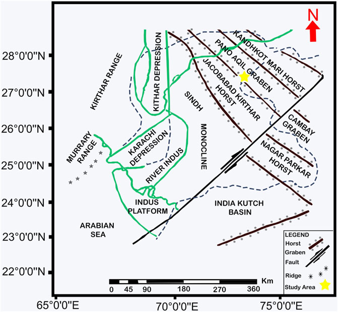
FIGURE 1. Location of the study area with major tectonic features in the surrounding, (modified after Saif-Ur-Rehman et al. 2016).
The cretaceous LGF was deposited in a shallow marine deltaic environment, during sea-level low stand as detached medium-to-coarse–grained sediments on the top of the distal (shale and siltstone) sediments of the previous high stand system tract (Berger et al., 2009). These sands exhibit characteristics similar to those of Indian shields in the neighborhood (Ahmad et al., 2007). The Cretaceous Sembar Formation serves as a confirmed source rock, with interbedded LGF and Upper Goru Formation shales serving as seal rock (Abbasi et al., 2016). Numerous large and enormous fields, including Miano, Sawan, and Mari, have been discovered in this roughly north–south reservoir fairway (Dar et al., 2021).
Materials and methods
This study incorporated wireline logs and well tops from four wells (Kadanwari-01, Kadanwari-03, Kadanwari-10, and Kadanwari-11) in the 3-D seismic volume of the study area. Except for a few problems, the data quality was fair for all mandatory log curves. For example, the RHOB curve was compromised in Kadanwari-01 well by poor borehole condition, that is, washout, while DTS was only recorded in Kadanwari-03 well. The Castagna relationship, which is an empirical link between compressional and shear velocities, was initially used to estimate the DTS log in wells with missing DTS (Castagna et al., 1985).
Well log constraints such as low RHOB and missing DTS curve have been addressed using the traditional rock physics method, which needs comprehensive petrophysical analysis, in situ reservoir parameters, and petro-elastic models as an input data set (Figure 2A). ML, on the other hand, has only used raw logs as input data from available wells, that is, GR, DT, DTS, LLD, and NPHI, which are divided into test and training data sets. The test data consist of log curves from the well where the DTS must be predicted, whereas the training data consist of log curves from wells that are involved in the DTS prediction process. Multiple SML methods, such as RF, DTR, and SVR, were used to train the data set (seismic and well), with the best algorithm (based on R2 and MAPE values) being used to derive elastic and petrophysical attributes (Figure 2B).
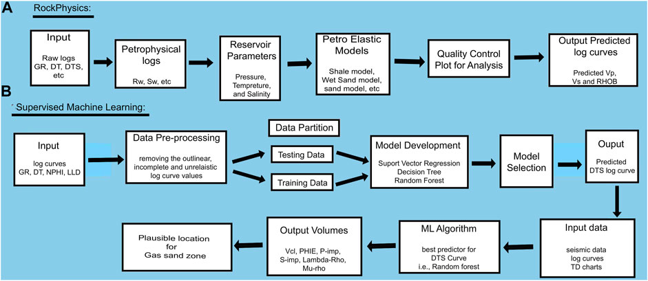
FIGURE 2. (A) Steps for conventional rock physics modeling workflow, and (B) SML procedure for prediction of DTS along with other elastic, and petrophysical attributes.
Rock physics modeling
The litho-facies were identified based on petrophysical cutoff values (Table 1), and then, a comprehensive rock physics model was developed by utilizing petro-elastic models (PEMs). The PEMs for shale, wet, and gas sands are generated in HampsonRussels software, incorporating reservoir in situ properties along with elastic constants of identified litho-facies (Table 2) (Miraj et al., 2021).
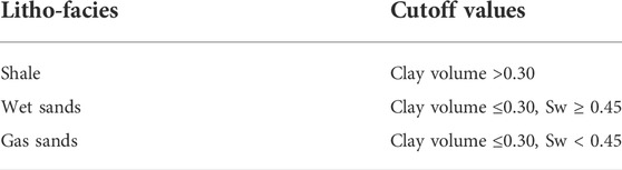
TABLE 1. Identified litho-facies based on the petrophysical cutoff values.

TABLE 2. Petrophysical and elastic properties of the reservoir utilized in PEMs.
The rock physics modeled elastic logs rectified the abnormal values, especially in poor RHOB, which is affected by bad borehole conditions (Figure 3A), and also predicted a reliable DTS curve (Figure 3A). The quantitative QC plots of modeled and measured DTP and DTS curves revealed consistent behavior along the central line (zero-error), while the RHOB deviated as the measured RHOB contained erroneous values (Figure 3B).
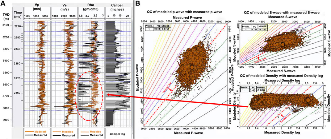
FIGURE 3. (A) Modeled Vp and Vs logs follow the measured log trend, whereas density log shows mismatch due to poor borehole condition highlighted through polygon, also illustrated by caliper log, and (B) QC cross plot displaying log points aligned at the central line for Vp and Vs; however, RHOB shows deviation due to error in wellbore measurement.
Supervised machine learning
ML has emerged as a new way to approach technical problems, that is, unrecorded logs of wellbore or deficiencies in measured logs, by analyzing and generating reliable logs (Liu et al., 2021). SML is the basic technique of ML, and its algorithms create a model to link the data (or feature) vector to a matching label or target vector using training data when both the input and the related label are known and provided to the algorithm (Litjens, 2017). Log curve prediction or correction is the part of the regression model used to forecast the continuous numerical variables (Liu et al., 2021).
Before training with the selected model, unrealistic or incomplete data points were eradicated from selected log curves. Outliers were defined as data points with a value that was away from the mean of the data by three times the standard deviation. After removing the outliers, the statistical properties of log curves used as test and training data sets are illustrated in Tables 3, 4.
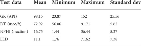
TABLE 3. Statistical description of the test data (Kadanwari-03).

TABLE 4. Statistical description of the training data (average out of three wells, i.e., Kadanwari-01, -10, and -11).
The log curves used to predict the DTS curve are displayed in the form of heat maps that provide the log values against subsurface depth through various color shades (Figure 4), demonstrating that the data are clear and smooth without any unrealistic values.
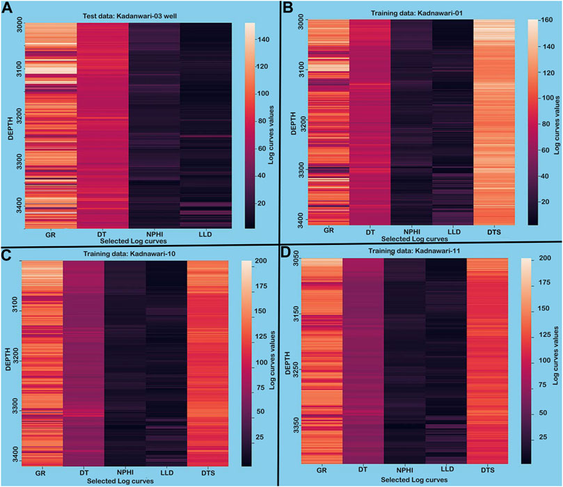
FIGURE 4. Heat map depicting values for selected logs against subsurface depth demonstrates that the data set is smooth and does not carry unrealistic values.
The DTS curve was only accessible in the Kadanwari-03 well; so, it had to be predicted in other wells by establishing a relationship with measured logs. The empirically derived DTS curve is used as training data by following the major procedures, which involve writing Python code, employing the most commonly used SML algorithms such as RF, DTR, and SVR with “scikit-learn” (Pedregosa et al., 2011), and to develop a Python framework (Figure 2). The best algorithm for the prediction among the applied algorithms is labeled based on R2 and MAPE values.
The SVR method is used for regression analysis (Chen et al., 2020), and it estimates real values using the kernel function (Steinwart, 2008) and predicts rock properties (Kang and Wang, 2010). An Ɛ-tube is introduced around the function that best approximates the continuous-value function f(x) in SVR and tries to balance model complexity and prediction error (Figure 5A) by assessing multiple kernel functions, values for kernel option, epsilon, and regularization. The DTR algorithm tackles regression problems using a tree structure, with the root node representing the sample data, interior nodes and branches displaying data attributes and decision rules, and leaf nodes expressing the outcome (Figure 5B). DTR has several advantages, including minimal data cleansing, non-linear performance, and a small number of hyperparameters to tune. The RF approach handled the over-fitting problem with decision trees.
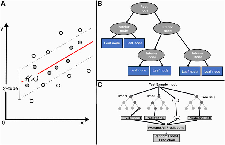
FIGURE 5. Supervised machine learning algorithms: (A) support vector regression (modified after Naganathan and Babulal, 2019), (B) decision tree regression (modified after Charbuty and Abdulazeez, 2021), and (C) random forest (modified after Rudd, 2020).
RF as a combination of multiple individual decision trees (Figure 5C) acted as an ensemble where multiple learners were trained to solve the complex relationships by voting among a collection (“forest”) of randomized decision trees (Breiman, 2001). The RF algorithm offered an advantage over opaque approaches, such as neural networks, which required a large number of hyperparameters to be tuned. RF has had a wide range of applications in solid earth geoscience (Bergen et al., 2019).
The missing DTS log was generated in the remaining wells using the aforementioned ML algorithms. To verify the adopted approach for DTS prediction, the predicted DTS logs (Kadanwari-01, -10, and -11) were combined to predict the DTS in the Kadanwari-03 well while keeping the measured DTS curve blind in Kadanwari-03 well. Figure 8 depicts the accuracy of the prediction, that is, the modeled log for Kadanwari-03 is in good agreement with the measured DTS, while in other wells, the predicted DTS and empirically derived DTS also delineate similarities in trends.
The RF algorithm, the best algorithm to predict the DTS curve based on R2 and MAPE, has been further employed to establish the relationship between the seismic amplitude of PSTM volume and well logs for estimating elastic and petrophysical properties. For the plausible gas sand location, the elastic properties (Zp, Zs, and λ-μ relation) and petrophysical properties (PHIE and Vcl) were mapped within the reservoir, that is, E-sands.
Results and discussion
The missing DTS log curve in Kadanwari-01, -03, -10, and -11 wells was predicted using traditional methods such as rock physics and by employing the algorithms of the most recent technique of SML such as RF, DTR, and SVR. These wells contain mandatory logs along with important information such as formation tops, time–depth relationships, and lithological information. For the identification of plausible sands, all wells are utilized for petrophysical interpretation and formation evaluation. To establish a petro-elastic relationship, rock physics bridges the gap between elastic and petrophysical properties.
Many researchers have successfully used rock physics techniques in the past to predict the DTS log in various fields such as the Middle Indus Basin (Azeem et al., 2015), Barnett Shale Formation (Guo and Li, 2015), North Poland (Wawrzyniak-Guz, 2019), LIB (Durrani et al., 2020), Zamzama Gas Field (Khan et al., 2021), and Mehar Block (Shakir et al., 2021) and further utilized these techniques in improving reservoir characterization based on seismic inversion techniques. Rock physics modeling has provided a decent estimation of the DTS curve, which was evaluated statistically through a QC plot, that is, prediction quality, which assesses the quality of the match between predicted and measured logs ranging from 0 to 1, was equal to 0.78 (Figure 3B). Another QC factor is the normalized root mean square error (NRMSE), which deals with the degree of difference, such as 0 for identical curves and 2 for the greatest difference, which was equal to 0.11 (Figure 3B). The abnormal values of RHOB (minimum of 1 gm/cc) at a depth of 3,500–3,820 m are rectified by the modeled logs that bring the ranges to the standard of the clastic reservoir (2.3–2.6 g/cc) (Figure 3B). Despite the reliable results of rock physics modeling, it is highly subject to the number of interdependent procedures, and if some error arises, it floats up to the final output. For example, the miscalculations made in petrophysical properties are added into petro-elastic models built for the facies and hence deteriorate the rock physics–modeled properties. Different procedures are incorporated into rock physics that need experts to find the exact reservoir properties, and it also increases the process cost.
On other hand, ML appeared to be a successful tool capable of constructing a relationship between log curves based on their effective features for DTS prediction to evaluate the reservoir properties. Many researchers have recently used ML for predicting the DTS curve, that is, Bukar et al. (2019), Anemangely et al. (2019), Miah (2021), Gamal et al. (2022), Gupta et al. (2019), and Liu et al. (2021). Due to complex reservoir attributes and limited data set, ML is a critical and optimized tool in the most productive LIB for predicting the DTS curve. This technique was developed for the first time to get maximum information from the produced well locations with missing DTS logs.
The accuracy of the predicted DTS curve is evaluated through R2 and MAPE (Saad et al., 2018). For Kadanwari-03 well, the only well having DTS run in its wellbore, RF proved to be the best algorithm for prediction with high values for R2 and low values for MAPE between predicted and measured DTS (Tables 5, 6). In the remaining wells, that is, Kadanwari-01, -10, and -11, the missing DTS is calculated by empirical relation and correlated with the predicted DTS log for comparison (Tables 5, 6). The SVR algorithm’s accuracy was reduced overall, even though it provided the same R2 value in Kadanwari-03 and -10, but its values decreased in Kadanwari-01 and -11, that is, 0.57 and 0.69, and MAPE values were overall higher, that is, 4.96, 2.16, 5.04, and 4.8 for all wells. The DTR algorithm proved to be the least accurate in DTS prediction, with the lowest values of R2, that is, 0.11, 0.52, 0.25, and 0.49, and highest values of MAPE, that is, 8.33, 4.76, 7.62, and 6.53 in Kadanwari-01, -03, -10, and -11, respectively. Few researchers have successfully utilized the RF approach for DTS prediction, that is, Gamal et al. (2022) employed RF for building sonic prediction models in complex lithology rocks including sandstone, limestone shale, and carbonate formations. The RF model accuracy was checked in comparison with the DTR approach through the correlation coefficient (R), that is, 0.986 for RF and 0.93 for DTR, and an average absolute percentage error (AAPE) of 1.12% for RF and 1.95% for DTR between actual values and predicted model. Gupta et al. (2019) have compared several machine learning regression techniques, such as multilinear regression (MLR), least absolute shrinkage and selection operator regression, support vector regression, random forest (RF), gradient boosting (GB), and alternating conditional expectations, to predict the synthetic sonic (Vp and Vs) and mechanical properties. Their results showed RF and GB as the best predictors with low uncertainties in the prediction, with R2 and adjusted R2 around 0.95 and RMS error around 0.18.
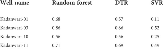
TABLE 5. Values of R2 between predicted and measured DTS curves.
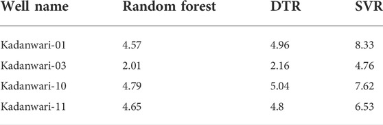
TABLE 6. Values of MAPE between predicted and measured DTS curves.
The correlation between the measured and predicted DTS curves is displayed through cross plots, that is, x-axis (measured/empirical DTS), y-axis = predicted DTS, and Z = depth values (3,000–3,450 m). The cross plots show the correlation of the applied ML technique at each well by observing the curve values along the zero-error line. This correlation also clearly shows that the RF technique performed efficiently and shows maximum alignment with centerline (Figures 6, 7).
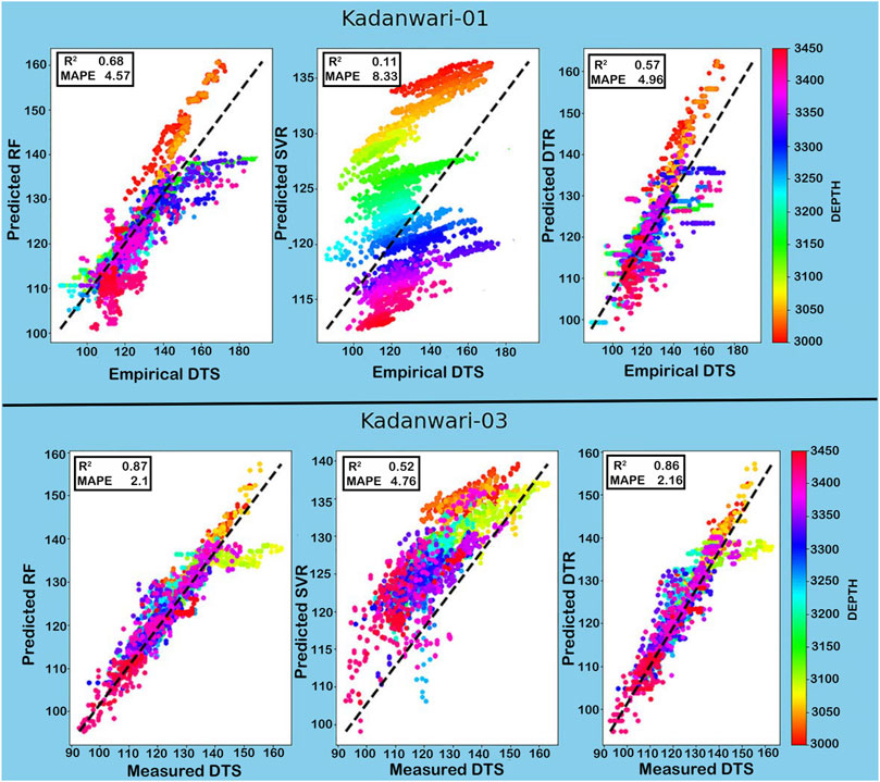
FIGURE 6. Cross plot between empirically derived and predicted DTS curve in the Kadanwari-01 well and between measured and predicted DTS curve in Kadanwari-03 depicting RF as the best algorithm.
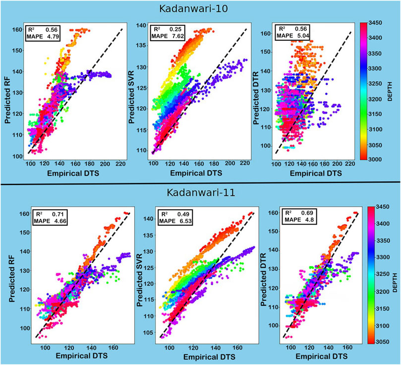
FIGURE 7. Cross plot between predicted and empirically derived DTS curves in Kadanwari-10 and -11 wells depicting RF as the best algorithm for DTS curve prediction.
The predicted DTS curve using various techniques, such as RF, SVM, and DTR, overlapped with the measured DTS for Kadanwari-03 and empirically derived DTS in other wells to evaluate the trends and curve ranges (Figure 8). In comparison to the DTR and SVR algorithms, the RF algorithm was more accurate in dealing with the heterogeneous reservoir sands of LGF (Dar et al., 2021), as it predicted DTS curves that were more consistent with measured curves across all wells (Figure 8).
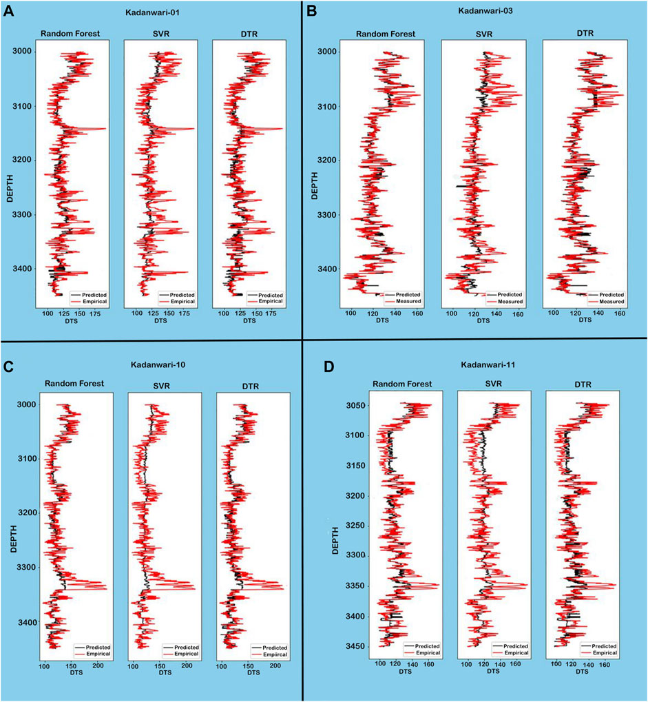
FIGURE 8. Comparison of trends between measured and predicted DTS curves depicts that RF is the most efficient technique.
The RF algorithm further utilizes the predicted DTS log, along with other significant elastic logs such as DTP and RHOB, to build a relationship with the 3-D seismic volume of the study area. This relationship was trained to predict elastic (Zp, Zs, λρ, and μρ) and petrophysical (PHIE and Vcl) attribute volumes. The maps generated by taking the average values within reservoir E-sands exhibited low values of Zp (10,400–10,800 gm/cc*m/s), Zs (6,300–6,600 gm/cc*m/s), and Vcl (30%–40%) with high PHIE (8–10%) around the producing well, Kadanwari-01 (Figure 9). Such a response from elastic and petrophysical properties indicates a potential area with good sand quality (Khan et al., 2021), that is, around the producing Kadanwari-01 well and channelized potential sands bound by the polygon (Figure 9). Low values for λρ (27–30 GPa*g/cc) cross ponding to higher μρ (38–44 GPa*g/cc) also support the presence of gas sands around the Kadanwari-01 well and within the polygon (Figure 9). Low values of λρ indicate the compressibility of gas, while the rigidity of quartz is delineated by a high μρ value (Young and Tatham, 2007).
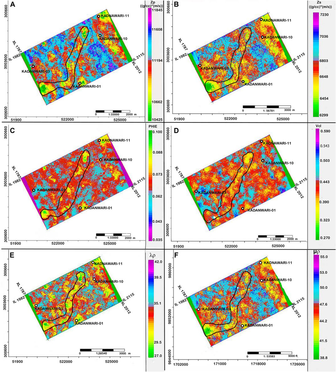
FIGURE 9. Average value maps extracted within E-sands exhibiting (A) low Zp, (B) low Zs, (C) high PHIE, and (D) low Vcl response around the producing Kadanwari-01, while polygon indicates plausible channelized gas sands, (E) λρ, and (F) μρ supporting the presence of gas sands at the same location.
Conclusion
Rock physics, a conventional but extensively used method, and ML, a new technology that employs artificial intelligence, are combined in this study to predict the missing DTS curve. However, the input data set and prerequisites for both approaches differ significantly. Rock physics, for example, demands petrophysical logs, reservoir in situ parameters, and petro-elastic models of the litho-facies identified in the area, all of which add time and cost to the operation. ML, on the other hand, is more accurate, faster, and less prone to errors, as well as able to work with a smaller data set. Three different SML algorithms, that is, RF, DTR, and SVR, are applied in the study, among which RF is proved to be more accurate in dealing with heterogeneous sand and it is further utilized for estimating elastic (Zp, Zs, λρ, and μρ) and petrophysical (PHIE and Vcl) volumes. In the stratigraphic slice extracted at the E-sand level, the reservoir in the area, gas sands zones were discovered with low Zp, Zs, and Vcl in contrast to higher PHIE which is also supported by the λ–μ relation with higher μλ corresponding to lower λρ values. Therefore, the ML technique will be effective in areas with missing log curve data, particularly in the LIB, which has older wells that lack DTS due to high drilling costs or insufficient drilling equipment at the time of drilling.
Data availability statement
The data used for this research work is highly confidential and it is property of the DGPC that provide this to university students for research work only. The permission will be required from DGPC to use it for the research purpose.
Author contributions
SA: conceptualization, methodology, and software. ML: supervision and writing—reviewing and editing. MH: visualization, investigation, and validation. ZK: data curation, formal analysis, and investigation.
Acknowledgments
The data were provided by the Directorate General for Petroleum Concession (DGPC), Pakistan, while software was provided by LMK Resources (Private) Limited, Islamabad, Pakistan and Compagnie Générale de Géophysique (CGG).
Conflict of interest
SA, MH, and ZK were employed by the company LMK Resources (Private) Limited.
The remaining author declares that the research was conducted in the absence of any commercial or financial relationships that could be construed as a potential conflict of interest.
Publisher’s note
All claims expressed in this article are solely those of the authors and do not necessarily represent those of their affiliated organizations, or those of the publisher, the editors, and the reviewers. Any product that may be evaluated in this article, or claim that may be made by its manufacturer, is not guaranteed or endorsed by the publisher.
References
Ahmad, N., Spadini, G., Palekar, A., and Subhani, M. A. (2007). Porosity prediction using 3D seismic inversion Kadanwari gas field, Pakistan. Pak. J. Hydrocarb. Res. 17, 95–102.
Ahmed Abbasi, S., Asim, S., Solangi, S., and Khan, F. (2016). Study of fault configuration related mysteries through multi seismic attribute analysis technique in Zamzama gas field area, southern Indus Basin, Pakistan. Geodesy Geodyn. 7, 132–142. doi:10.1016/j.geog.2016.04.002
Anemangely, M., Ramezanzadeh, A., Amiri, H., and Hoseinpour, S. A. (2019). Machine learning technique for the prediction of shear wave velocity using petrophysical logs. J. Petroleum Sci. Eng. 174, 306–327. doi:10.1016/j.petrol.2018.11.032
Avseth, P., Mukerji, T., and Mavko, G. (2010). Quantitative seismic interpretation: Applying rock physics tools to reduce interpretation risk. Cambridge, UK: Cambridge University Press, doi:10.1017/CBO9780511600074
Azeem, T., Chun, W. Y., MonaLisa, P., Khalid, L. X., Qing, M. I., Ehsan, M. J., et al. (2017). An integrated petrophysical and rock physics analysis to improve reservoir characterization of Cretaceous sand intervals in Middle Indus Basin, Pakistan. J. Geophys. Eng. 14 (2), 212–225. doi:10.1088/1742-2140/14/2/212
Bai, Y., and Tan, M. (2021). Dynamic committee machine with fuzzy-c-means clustering for total organic carbon content prediction from wireline logs. Comput. Geosciences 146, 104626. doi:10.1016/j.cageo.2020.104626
Bergen, K. J., Johnson, P. A., de Hoop, M. V., and Beroza, G. C. (2019). Machine learning for data-driven discovery in solid Earth geoscience. Science 363 (6433), eaau0323. doi:10.1126/science.aau0323
Berger, A., Gier, S., and Krois, P. (2009). Porosity-preserving chlorite cements in shallow-marine volcaniclastic sandstones: Evidence from Cretaceous sandstones of the Sawan gas field, Pakistan. Bulletin 93 (5), 595–615. doi:10.1306/01300908096
Bukar, I., Adamu, M. B., and Hassan, U. (2019). “A machine learning approach to shear sonic log prediction,” in Proceedings of the SPE Nigeria Annual International Conference and Exhibition, Lagos, Nigeria, August 2019. doi:10.2118/198764-ms
Castagna, J. P., Batzle, M. L., and Eastwood, R. L. (1985). Relationships between compressional‐wave and shear‐wave velocities in clastic silicate rocks. geophysics 50 (4), 571–581. doi:10.1190/1.1441933
Charbuty, B., and Abdulazeez, A. (2021). Classification based on decision tree algorithm for machine learning. J. appl. sci. technol. trends 2 (01), 20–28.
Chen, G., Chen, L., and Li, Q. (2020). Comparison and application of neural networks in LWD lithology identification. IOP Conf. Ser. Earth Environ. Sci.IOP Publ. 526 (1), 012146. doi:10.1088/1755-1315/526/1/012146
Chen, W., Yang, L., Zha, B., Zhang, M., and Chen, Y. (2020). Deep learning reservoir porosity prediction based on multilayer long short-term memory network. Geophysics 85 (4), WA213–WA225. doi:10.1190/geo2019-0261.1
Dar, Q. U. Z., Renhai, P., Ghazi, S., Ahmed, S., Ali, R. I., and Mehmood, M., (2021). Depositional facies and reservoir characteristics of the early cretaceous lower Goru Formation, lower Indus basin Pakistan: Integration of petrographic and gamma-ray log analysis. Petroleum. doi:10.1016/j.petlm.2021.09.003
Dornan, T., O'Sullivan, G., O'Riain, N., Stueeken, E., and Goodhue, R. (2020). The application of machine learning methods to aggregate geochemistry predicts quarry source location: An example from Ireland. Comput. Geosciences 140, 104495. doi:10.1016/j.cageo.2020.104495
Durrani, M. Z. A., Talib, M., and Sarosh, B. (2020). Rock physics-driven quantitative seismic reservoir characterization of a tight gas reservoir: A case study from the lower Indus basin in Pakistan. First Break 38 (11), 43–53. doi:10.3997/1365-2397.fb2020079
Ehsan, M., Gu, H., Akhtar, M. M., Abbasi, S. S., and Ehsan, U. (2018). A geological study of reservoir formations and exploratory well depths statistical analysis in Sindh Province, Southern Lower Indus Basin, Pakistan. Kuwait J. Sci. 45 (2), 84–93.
Feng, R., Mejer Hansen, T. M., Grana, D., and Balling, N. (2020). An unsupervised deep-learning method for porosity estimation based on poststack seismic data. Geophysics 85 (6), M97–M105. doi:10.1190/geo2020-0121.1
Gamal, H., Alsaihati, A., and Elkatatny, S. (2022). Predicting the rock sonic logs while drilling by random forest and decision tree-based algorithms. J. Energy Resour. Technol. 144, 043203. doi:10.1115/1.4051670
Grana, D., Azevedo, L., and Liu, M. (2020). A comparison of deep machine learning and Monte Carlo methods for facies classification from seismic data. Geophysics 85 (4), WA41–WA52. doi:10.1190/geo2019-0405.1
Guo, Z., and Li, X. Y. (2015). Rock physics model-based prediction of shear wave velocity in the Barnett Shale formation. J. Geophys. Eng. 12 (3), 527–534. doi:10.1088/1742-2132/12/3/527
Gupta, I., Devegowda, D., Jayaram, V., Rai, C., and Sondergeld, C. (2019). Machine learning regressors and their metrics to predict synthetic sonic and mechanical properties. Interpretation 7 (3), SF41–SF55. doi:10.1190/INT-2018-0255.1
Gupta, R., Srivastava, D., Sahu, M., Tiwari, S., Ambasta, R. K., and Kumar, P., (2021). Artificial intelligence to deep learning: Machine intelligence approach for drug discovery. Mol. Divers. 25 (3), 1315–1360. doi:10.1007/s11030-021-10217-3
Hall, B. (2016). Facies classification using machine learning. Lead. Edge 35 (10), 906–909. doi:10.1190/tle35100906.1
Hamada, G. M. (2004). Reservoir fluids identification using Vp/Vs ratio? Oil Gas Sci. Technol. - Rev. IFP 59 (6), 649–654. doi:10.2516/ogst:2004046
Han, D. H. (1987). Effects of porosity and clay content on acoustic properties of sandstones and unconsolidated sediments (CA, USA: Stanford University). Doctoral dissertation.
Jakobsen, M., Hudson, J. A., and Johansen, T. A. (2003). T-matrix approach to shale acoustics. Geophys. J. Int. 154 (2), 533–558. doi:10.1046/j.1365-246X.2003.01977.x
Kang, Y., and Wang, J. (20102010). A support-vector-machine-based method for predicting large-deformation in rock mass. Seventh Int. Conf. Fuzzy Syst. Knowl. Discov. 3, 1176–1180. doi:10.1109/FSKD.2010.5569148
Kazmi, A. H., and Jan, M. Q. (1997). Geology and tectonics of Pakistan. Oregon, USA: Graphic publishers.
Khan, Z. U., Lisa, M., Hussain, M., and Ahmed, S. A. (2021). Gas-bearing sands appraisal through inverted elastic attributes assisted with PNN approximation of petrophysical properties. Kuwait J. Sci. doi:10.48129/kjs.15915
Litjens, G., Kooi, T., Bejnordi, B. E., Setio, A. A. A., Ciompi, F., Ghafoorian, M., et al. (2017). A survey on deep learning in medical image analysis. Med. image Anal. 42, 60–88. doi:10.1016/j.media.2017.07.005
Liu, S., Zhao, Y., and Wang, Z. (2021). Artificial intelligence method for shear wave travel time prediction considering reservoir geological continuity. Math. Problems Eng. 2021, 5520428–18. doi:10.1155/2021/5520428
Miah, M. I. (2021). Improved prediction of shear wave velocity for clastic sedimentary rocks using hybrid model with core data. J. Rock Mech. Geotechnical Eng. 13 (6), 1466–1477. doi:10.1016/j.jrmge.2021.06.014
Miraj, M. A. F., Javaid, H., Ali, N., Javaid, P. W. S., Rathore, R. F., Ahsan, N., et al. (2021). An integrated approach to evaluate the hydrocarbon potential of jurassic samana suk formation in Middle Indus basin, Pakistan. Kuwait J. Sci. 48 (4), 1–11. doi:10.48129/kjs.v48i4.9193
Mohammed, M., Khan, M. B., and Bashier, E. B. M. (2016). Machine learning: Algorithms and applications. Boca Raton, Florida: CRC Press. doi:10.1201/9781315371658
Munyithya, J. M., Ehirim, C. N., and Dagogo, T. (2019). Rock physics models and seismic inversion in reservoir characterization, “MUN” onshore Niger delta field. Ijg 10 (11), 981–994. doi:10.4236/ijg.2019.1011056
Naganathan, G. S., and Babulal, C. K. (2019). Optimization of support vector machine parameters for voltage stability margin assessment in the deregulated power system. Soft Computing 23 (20), 10495–10495. doi:10.1007/s00500-018-3615-x
Pedregosa, F., Varoquaux, G., Gramfort, A., Michel, V., Thirion, B., Grisel, O., et al. (2011). Scikit-learn: Machine learning in Python. J. Mach. Learn. Res. 12, 2825–2830.
Saif-Ur-Rehman, K. J., Mehmood, M. F., Shafiq, Z., and Jadoon, I. A. (2016). Structural styles and petroleum potential of Miano block, central Indus Basin, Pakistan. Ijg 7 (10), 1145–1155. doi:10.4236/ijg.2016.710086
Rudd, J. M. (2020). “An Empirical Study of Downstream Analysis Effects of Model Pre-Processing Choices. Open journal of statistics 10 (5), 735–809. doi:10.4236/ojs.2020.105046
Saad, B., Negara, A., and Syed Ali, S. (2018). “Digital rock physics combined with machine learning for rock mechanical properties characterization,” in Proceedings of the Abu Dhabi International Petroleum Exhibition & Conference, Abu Dhabi, UAE, November 2018. doi:10.2118/193269-MS
Shakir, U., Ali, A., Amjad, M. R., and Hussain, M. (2021). Improved gas sand facies classification and enhanced reservoir description based on calibrated rock physics modelling: A case study. Open Geosci. 13 (1), 1476–1493. doi:10.1515/geo-2020-0311
Song, S., Hou, J., Dou, L., Song, Z., and Sun, S. (2020). Geologist-level wireline log shape identification with recurrent neural networks. Comput. Geosciences 134, 104313. doi:10.1016/j.cageo.2019.104313
Steinwart, I., and Christmann, A. (2008). Support vector machines. Berlin, Germany: Springer Science & Business Media.
Wawrzyniak-Guz, K. (2019). Rock physics modelling for determination of effective elastic properties of the lower Paleozoic shale formation, North Poland. Acta Geophys. 67 (6), 1967–1989. doi:10.1007/s11600-019-00355-6
Keywords: DTS log prediction, supervised learning, random forest, rock physics modeling, petrophysics, reservoir characterization
Citation: Ahmed SA, MonaLisa , Hussain M and Khan ZU (2022) Supervised machine learning for predicting shear sonic log (DTS) and volumes of petrophysical and elastic attributes, Kadanwari Gas Field, Pakistan. Front. Earth Sci. 10:919130. doi: 10.3389/feart.2022.919130
Received: 13 April 2022; Accepted: 29 June 2022;
Published: 12 August 2022.
Edited by:
Amin Beiranvand Pour, INOS University Malaysia Terengganu, MalaysiaReviewed by:
Mohamed Abdel-Fattah, University of Sharjah, United Arab EmiratesYasir Bashir, Universiti Sains Malaysia (USM), Malaysia
Copyright © 2022 Ahmed, MonaLisa, Hussain and Khan. This is an open-access article distributed under the terms of the Creative Commons Attribution License (CC BY). The use, distribution or reproduction in other forums is permitted, provided the original author(s) and the copyright owner(s) are credited and that the original publication in this journal is cited, in accordance with accepted academic practice. No use, distribution or reproduction is permitted which does not comply with these terms.
*Correspondence: Syed Adnan Ahmed, c2FkbmFuODRAaG90bWFpbC5jb20=