Discrete Bubble Flow in Granular Porous Media via Multiphase Computational Fluid Dynamic Simulation

The coal seam gas industry has raised public concerns about the potential risk of groundwater contamination, where gases leaked from coal seams are thought to pollute groundwater. However, the basic principles and controlling parameters for gas seepage from deep ground formations to the ground surface have not been fully understood. As a possible mechanism for gas transport in the subsurface environment, discrete bubble flow was previously investigated using laboratory experiments by Ma et al. (Water Resour. Res, 2015, 51 (6), 4359–4373). This study developed a multiphase computational fluid dynamic (CFD) model to simulate discrete bubbly flow in a two-dimensional granular porous media at the pore scale. Following the experimental setup from Ma et al. (Water Resour. Res, 2015, 51 (6), 4359–4373), a “point source” with preset bubble fluxes was specified in a simulating domain representing the flume size in the earlier experiments. There were around 7,000 granular particles within this domain to model the porous media. This numerical model was validated by conserving the gas mass in the simulating domain. The simulation results provide more physical insights into complex bubble transport behaviour in porous media through specific plume parameters. The breakthrough time of the bubble plume and the cross-sectional averaged velocity of ambient pore water flow were manifested to be proportional to the gas release rates in the logarithmic scales. Also, the bubble plume width was also observed to be proportional to the gas release rates. Moreover, the gas distribution on the top boundary could be observed. The outcomes were further tested against the scaling solutions proposed by Ma et al. (Water Resour. Res, 2015, 51 (6), 4359–4373) with disagreements. The limitations of this multiphase computational fluid dynamic model were finally discussed.

Introduction

The coal seam gas industry has raised public concerns about the potentially high risk of potential groundwater pollution, where gases leaked from coal seam beds are prone to contaminate groundwater (Charbeneau and Sherif, 2002). In addition, those light hydrocarbon gases in high concentrations, such as ethane, methane, propane, etc., can transport in hydrocarbon gas-storing rock mass, particularly in preferential flow paths comprised of fracture and fault zones (Duddridge et al., 1991; Annunziatellis et al., 2008). Therefore, soil gas concentration anomalies in the topsoil are primarily attributable to those gas migration in the following mechanisms: 1) gas diffusion; 2) the dissolved gas carried by groundwater flow; 3) continuous gas phase driven by pressure gradient; and 4) bubbly flow transport (Kristiansson and Malmqvist, 1984). Although many studies have comprehensively studied the former three mechanisms (Fleischer and Mogro-Campero, 1978, 1979; Saunders et al., 1999), the basic principles and controlling parameters for bubbly flow from deep ground formations to the ground surface, proposed by Etiope and Martinelli (2002), have not been comprehensively investigated and developed. This research objective is, so far, still at an initial stage with a few academic attempts (Ma, 2015; Mahabadi et al., 2018; Chang and Lindquist, 2020; Yi et al., 2022).

A conceptual model in Figure 1 illustrates subsurface microbubble transport processes, where bubbles were transported in the fracture, which acted as the point source of gas for the soil layer. The discrete bubble transport mechanism is not well understood, especially in the saturated shallow soils near the ground surface. This water-saturated porous media could act as a buffer zone for gas bubbles percolating through the basement rock and modifying bubble transport behaviour. Hence, soil gas concentration signals could be detected at the ground surface. Ma et al. (2015) has successfully carried out quasi-two-dimensional (2D) physical modelling to explore potential buffering effects to study microbubble migration and ambient groundwater circulation. A scaling solution, accounting for bubble injection rate, bubble plume tip velocity, width and breakthrough time of the plume front, was also established by Ma et al. (2015). As a continuous work after this former study, we further performed 2D numerical modelling to simulate the transport process of discrete bubbles with a localized source of gas bubbles at the bottom boundary of the saturated soil later. This “point” source models the input condition provided by gas flow through fractures underlying the water-saturated soil layer. Based on these simulation outcomes, it is expected that more physical insights could be brought into complex bubble transport behaviour in porous media. Also, this work could adequately quantify both advective and dispersive bubble migrations for engineering practices.

FIGURE 1

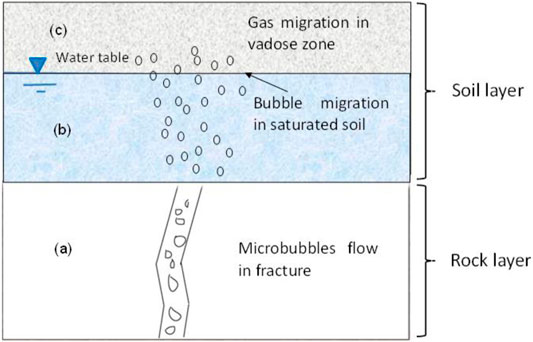
FIGURE 1. Conceptual model of the gas movement in the studied subsurface environment: (A) microbubble flow in a fracture; (B) bubble flow in the saturated soil layer; the microbubbles become more dispersive in the soil layer, and (C) gas transport in the vadose zone.

Literature Review of Numerical Models at Multiscale

Numerical simulations of gas transport in porous media have been extensively studied previously. This section reviews two conventional gas transport models: the continuum model of two-phase flow in porous media (Yan et al., 2022c) and the continuum “colloidal” discrete bubbles transport model (Ma, 2012) in order to identify their advantages and disadvantages. This review contributed to the development of a new model that could overcome those shortcomings.

The Model of Two-phase Flow in Porous Media

The two phases Darcy flow model treats both the water phase and gas phase as continuum phases (Bear, 1972). Depending on how much space each phase occupies, the two phases interact dynamically by the relative permeability and effective saturation. The governing equations for water and gas flow are given (Bear, 1972):

For the wetting phase (water):

$\nabla \cdot \left[\frac{k{k}_{r,w}}{{\mu }_w}\left(\nabla P_w+{\rho }_{w}g\nabla z\right)\right]=\varphi \frac{\mathit{\partial }S{e}_w}{\partial P_c}\frac{\partial \left(P_{nw}-P_w\right)}{\partial t};(1)$

For the nonwetting phase (gas):

$\nabla \cdot \left[\frac{k{k}_{r,nw}}{{\mu }_{nw}}\left(\nabla P_{nw}+{\rho }_{nw}g\nabla z\right)\right]=-\varphi \frac{\partial S{e}_w}{\partial P_c}\frac{\partial \left(P_{nw}-P_w\right)}{\partial t},(2)$

where subscript w is for the wetting phase (water phase); subscript nw is for the nonwetting phase (gas phase); z is the vertical coordinate, respectively; k is the media permeability [L²]; k_r is relative permeability for the wetting or nonwetting phase [-]; μ is the dynamic viscosity [M/TL]; ρ is fluid density [M/L³]; g is the magnitude of gravitational acceleration [L/T²]; Se is effective saturation (varying from 0 to 1), and P is the pressure [M/LT²]. The capillary pressure could be expressed as P_c = P_nw–P_w.

Specific capacity is defined as:

$C_w=-C_{nw}=\varphi \frac{\partial S{e}_w}{\partial P_c},(3)$

where C is the specific capacity [LT²/M] and $\varphi$ is the porosity [L³/L³]. The $\varphi$, C, Se, k and P_c vary simultaneously. Mualem (1976) and Van Genuchten (1980) applied the soil water retention and relative permeability functions to express changes in the $\varphi$, C, Se and k as functions of P_c. The capillary pressure was transformed to the equivalent water head as Hc= P_c/(ρ_water g).

The hydraulic properties relative to the wetting fluid are given below:

If Hc>0 (unsaturated zone):

$\begin{array}{l}{\varphi }_w={\varphi }_{r,w}+Se\left({\varphi }_{s,w}-{\varphi }_{r,w}\right)\\ S{e}_w=\frac{1}{{\left[1+{\left|\alpha Hc\right|}^n\right]}^m}\\ C_w=\frac{\alpha m}{1-m}\left({\varphi }_{s,w}-{\varphi }_{r,w}\right)S{e}_w^{\frac{1}{m}}{\left(1-S{e}_w^{\frac{1}{m}}\right)}^m\\ k_{r,w}=S{e}_w^L{\left(1-{\left(1-S{e}_w^{\frac{1}{m}}\right)}^m\right)}^2\end{array};(4)$

If Hc≤0 (saturated zone):

$\begin{array}{l}{\varphi }_w={\varphi }_{s,w}\\ S{e}_w=1\\ C_w=0\\ k_{r,w}=1\end{array};(5)$

For the nonwetting fluid:

$\begin{array}{l}{\varphi }_{nw}={\varphi }_{s,w}-{\varphi }_w\\ S{e}_{nw}=1-S{e}_w\\ C_{nw}=-C_w\\ k_{r,nw}={\left(1-S{e}_w\right)}^L{\left(1-S{e}_w^{\frac{1}{m}}\right)}^{2m}\end{array},(6)$

where ϕ_s is the total porosity; ϕ_r is the residual porosity to the total porosity; α, n, m and L are the Van Genuchten (1980) parameters, which depend on the soil type. These parameters could be determined using unsaturated soil tests, including standard tests and soil column tests (Yan et al., 2021a) with various unsaturated soil sensors (Yan et al., 2022a).

This approach described above can simulate continuous gas phase transport in the soil layer, driven by pressure. However, bubbles are driven by the buoyancy force and travel discretely in the porous media in terms of bubble migration. As a result, the gas relative permeability could not be applied to describe discontinuous bubble flow. Furthermore, this approach does not provide information on gas concentration, although bubble concentration is significant for interpreting the concentration mapping of soil gas. Therefore, different approaches to quantifying the microbubble flow are highly demanded and reviewed below.

The Continuum “Colloidal” Discrete Bubbles Transport

Price (1986) conducted qualitative experiments to study bubble flow in porous media, observing that large gas bubbles stuck to surfaces and were trapped at pore throats. These large bubbles then block the pathway of smaller rising bubbles. However, the bubbles considered in the present study are discrete bubbles in colloidal sizes. MacElvain, (1969) suggested that if bubbles are in colloidal sizes (in the range between 0.7 and 20 µm), Brownian motion will prevent them from sticking to the solid particle surfaces, and they could continue to move upward. Wan et al. (2001) tested this hypothesis using laboratory experiments to generate stable discrete bubbles and measure their transport properties in porous media. The results indicated that the surface interaction between sand grains and bubbles was not favourable for deposition. Under such surface interaction, bubbles can travel over significant distances in the subsurface environment. Furthermore, the individual gas bubbles can be seen as finite fluid particles within the liquid continuum. Therefore, microbubble transport in porous media may be treated as a particular case of colloid transport (Wan et al., 2001):

$R\frac{\partial C}{\partial t}=D\frac{{\partial }^{2}C}{\partial z^2}-v_o\frac{\partial C}{\partial z}-k_{a}C,(7)$

where C is the bubble concentration [M/L³]; R is the retardation factor for local sorption equilibrium; t is the time [T]; v_o is the gas velocity [L/T]; D is the dispersion coefficient [L²/T] and $k_a$ is the trapping coefficient. As for applying the above colloidal transport equation, an important question arises regarding defining the dispersion coefficient and the microbubble flow velocity. Every single bubble has an individual dispersion ability and velocity. In an infinite viscous media without walls or other particles, the bubble movement in static water is assumed to follow Stoke’s law [22], which is applied to calculate the bubble velocity given by

$v=d^{2}g\frac{{\rho }_w-{\rho }_g}{18\mu },(8)$

where ν is the bubble velocity relative to the water [L/T], d is the bubble diameter [L], ρ_w is the water density [M/L³], ρ_g is the gas density [M/L³], and µ is the dynamic viscosity of water [M/TL].

Stoke’s law is only applicable to small bubbles with an immobile surface. Eq 8 shows that the bubble velocity is directly related to the bubble diameter. The bubble radius grows when the hydrostatic pressure decreases, consequentially increasing bubble velocity. The bubble velocity given by Stokes’s law is only applicable to a single bubble motion. It does not consider interference by the other bubbles and the wall effect induced by the fracture/porous media.

When the bubbles come into close contact with walls, the terminal bubble velocities decrease. The viscous drag increases since the fluid, displaced by the rising bubble, is squeezed into a narrower cross-sectional area between the wall and particle, increasing the viscous resistance to flow. Happel and Brenner (1983), who investigated the wall effects on the motion of a single particle, found that the wall effects are minor if the particle size is significantly smaller than the aperture. The bubbles velocity within a narrow fracture/pore space, including the wall effect, can be described by the following equation (Brown, 2000):

$v_w/v=1-1.004\left(r/b\right)+0.418{\left(r/b\right)}^3-0.21{\left(r/b\right)}^4-0.169{\left(r/b\right)}^5,(9)$

where r is the bubble radius [L], b is half the size of the fracture aperture [L], $v_w$ is the bubble velocity [L/T] along the fracture and $v$ is Stoke’s velocity without wall effect [L/T].

The interplay of bubble rebound and coalescence could be necessary when a group of bubbles migrate in the form of bubble trains. The bubble coalescence and rebound are controlled by three actions: attractive surface forces, hydrodynamic interaction, and dynamic bubble collisions (Vakarelski et al., 2010). When gas fluxes increase, bubbles can coalesce and produce vertically elongated bubbles, called “slugs”, creating continuous gas streams within the porous media (Etiope and Martinelli, 2002). In general, the maximum size of a bubble is constrained by the minimum cross-section area of the flow pathway, such as the throat of the fracture/granular porous media. Várhegyi et al. (1986) established a model to estimate maximum bubble size as a function of the porosity and the grain size:

$d=1.26d_G\varphi \left(\varphi +0.21\right),(10)$

where $d$ is the bubble diameter [L]; $d_G$ is the mean grain size [L], and $\varphi$ is the media porosity.

This population colloidal microbubble transport model is efficient for modelling bubble flow in porous media. Nonetheless, this approach does not include the dynamic interaction between the bubble and ambient water flow. As prior experimental work by Ma et al. (2015) concluded, the ambient pore water flow may interact with bubble flow strongly.

Numerical Methodology

Multiphase Computational Fluid Dynamics

Considering the disadvantages of the aforementioned two models, we selected a two-phase bubbly flow model for this study. This pore-scale two-phase flow model described by the Navier-Stokes equation can simulate the buoyancy force and the dynamic interaction between bubbles and water. A numerical model using COMSOL Multiphysics engineering simulation software is developed. COMSOL is a finite element simulation software (Li et al., 2009). It originated from the MATLAB toolbox and has been well integrated with MATLAB, which provides convenience for pre-processing and post-processing. The program has been applied and tested extensively for a wide range of gas transport problems in saturated and vadose zones (Abreu and Johnson, 2005; You et al., 2011). A pore-scale numerical model was conducted to simulate bubbly flow in a two-dimensional (2D) porous media, equivalent to the laboratory geophysical modelling published by Ma et al. (2015). Compared to other two-phase flow models simulating the gas phase in continuous form (Yan et al., 2021b; Yan et al., 2022b), this model can simulate discrete bubbles without coalescence.

Continuum models with mass and momentum conservation equations describe two-phase bubbly flow in porous media at the pore scale. Mass conservation (continuity) equations:

$\frac{\partial }{\partial t}\left({\varphi }_l{\rho }_l\right)+\nabla \cdot \left({\varphi }_l{\rho }_l{u}_l\right)=0;(11)$

$\frac{\partial }{\partial t}\left({\varphi }_g{\rho }_g\right)+\nabla \cdot \left({\varphi }_g{\rho }_g{u}_g\right)=0.(12)$

Momentum conservation equations (Navier–Stokes equation):

$\frac{\partial }{\partial t}\left({\varphi }_l{\rho }_l{u}_l\right)+{\varphi }_l{\rho }_l{u}_l\cdot \nabla u_l=-{\varphi }_l\nabla p+{\varphi }_l{\rho }_{l}g+\nabla \cdot \left[{\varphi }_l{\mu }_l\left(\nabla u_l+\nabla u_l^t\right)\right],(13)$

where subscript $l$ denotes a liquid phase; subscript g denotes a gas phase; $\rho$ is the density; $\varphi$ is the phase volume fraction; $u$ is the phase velocity; µ is the dynamic viscosity; $p$ is the phase pressure; $\frac{\partial }{\partial t}\left(\varphi \rho u\right)$ is the local acceleration term; $\varphi \rho u\cdot \nabla u$ is the convective acceleration term; $\varphi \nabla p$ is the pressure gradient; $\varphi \rho g$ is the gravitational force and $\nabla \cdot \left[\varphi \mu \left(\nabla u+\nabla u^T\right)\right]$ is the viscosity force.

This numerical work follows the previous experimental setup from Ma et al. (2015). The released bubbles remained spherical shape (the bubble size is around 300 µm) through the experiments and were about one order of magnitude smaller than hydrogel beads. In addition, no trapping and attachment of bubbles to solid matrixes were visually observed. Consequently, there is no direct contact between gas and solid matrixes throughout the experiments, leading to no capillary actions involving solid matrixes. Accordingly, capillary effects are not included in the bubble transport numerical model. Therefore, the Navier-Stokes equation is adequate and appropriate to simulate ambient pore water flow around discrete bubble transport. The discrete bubbles were simulated as spherical particles floating upward following a gas bubble model described by Eqs 14–17.

According to the mass and momentum conservation equation, $u_g$ could be calculated as

$u_g=u_l+u_{slip},(14)$

where $u_{slip}$ is the velocity difference between the gas phase and liquid phase. The drag force exerted on each bubble is given by Crowe et al., 1998).

$\frac{3}{4}\frac{C_d}{d_b}{\rho }_l|u_{slip}|u_{slip}=-\nabla p,(15)$

where $C_d$ is the drag force and $d_b$ is the diameter of the bubbles (Kitanidis, 1997; Crowe et al., 1998; Clift et al., 2005). The Hadamard-Rybczynski formula (Hadamard, 1911; Rybczynski, 1911) can be applied to calculate $C_d$ :

$C_d=\frac{16{\mu }_l}{d_b{\rho }_l{u}_{slip}}.(16)$

The gas density is calculated from the ideal gas laws:

${\rho }_g=\frac{pM}{RT},(17)$

where p is the pressure of the gas, M is the amount of substance of gas, R is the universal gas constant, and T is the absolute temperature of the gas. The relationship between the gas volume fraction and liquid volume fraction is:

${\varphi }_l+{\varphi }_g=1.(18)$

Numerical Simulation Setup and Settings

As shown in Figure 2, a two-dimensional water-saturated domain was created with the dimensions of 700×900 mm² (width $\times$ height), the same size as the experimental flume from Ma et al. (2015). There are approximately 7,000 spherical particles preset in the domain in order to simulate the transparent granular soil as a porous media (Yan et al., 2022d), which yields a porosity of 0.494. All solid particles were not movable and rotatable. Then, a sequential sphere packing method was applied to establish the pore-scale domain. This packing method employs trilateration equations to pack spheres with a predefined grain size distribution (GSD of hydrogel beads) and a given porosity (To et al., 2016). In addition, the boundary conditions are specified, as shown in Figure 2.

FIGURE 2

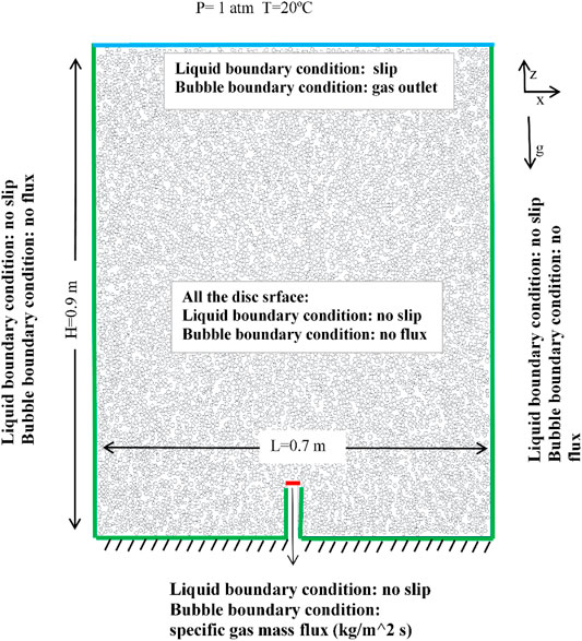
FIGURE 2. Schematic sketch of geometry and boundary conditions for the current numerical study: no-water flow boundary conditions for the domain bottom boundary, the no-slip solid side boundaries and particle surface; specified gas flux is set as the bubble gas diffuser point (red line at the bottom).

A series of numerical experiments with different gas release rates $\left(Q\right)$ of 5, 10, 20 and 30 ml/min were conducted. The gas inlet diffuser is a gas flux boundary. Thus, the gas release rates were converted into the gas flux of $1.78\times {10}^{-4}$ , $3.57\times {10}^{-4}$ , $7.15\times {10}^{-4}$ and $11\times {10}^{-4}$ kg/(m²·s) corresponding to the gas release rates and bubble diffuser setting applied in the laboratory experiments by Ma et al. (2015).

Results and Discussion

Validation of Mass Conservation

In order to test the model performance, mass conservation is examined. As shown in Figure 3, the total gas flux at the top boundary of the domain was plotted over time with different gas release rates. The evolution of the gas flux over time exhibits a rapid increase and sharp overshoots in the initial stage. After the gas breakthrough, gas fluxes were stabilized and kept at a plateau under steady-state conditions. The overshoot could be caused by massive ambient gas transporting together with a bubble plume during a short time right after the gas breakthrough, but this local disturbance quickly fades away. Although the input gas fluxes are labelled for different gas release rates on each curve, they all match well with gas output fluxes at the steady-state conditions. Therefore, the model is manifested to be mass conservative.

FIGURE 3

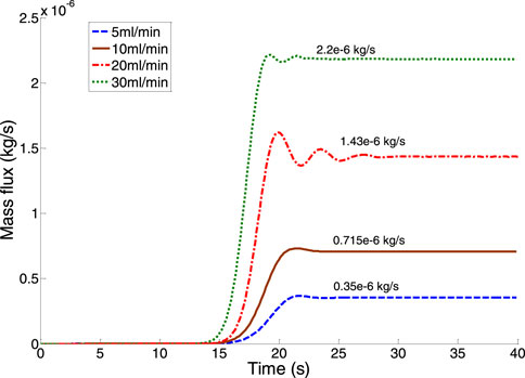
FIGURE 3. Evolution of gas mass flux on the top boundary over time.

Bubble Plume Width Development

In order to examine results simulated by the numerical models in comparison with the laboratory experiments carried out by Ma et al. (2015), the simulation results are analyzed following the procedure for analyzing the experimental data in the previous work (Ma et al., 2015). The width variations of the estimated bubble plume at the top of the domain against gas release rates $\left(W_{top}-Q\right)$ are shown in Figure 3A after the bubble plume breakthrough and reaching the steady-state conditions. The slope of the $W_{top}-Q$ trendline is 1.65, which is around 1.6 times that of the laboratory $W_{top}-Q$ trendline (slope = 1). Figure 4.

FIGURE 4

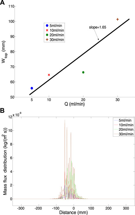
FIGURE 4. (A) The width of the bubble plume $\left(W_{top}\right)$ at the top boundary of the domain; (B) the gas mass flux distribution at the top boundary of the domain.

Gas flux distributions at the top boundary of the domain are plotted to understand this inconsistency. Figure 3B shows that the gas flux variation at the top boundary corresponds with the increasing gas release rate. The modelled $W_{top}$ is narrower than the laboratory results provided by Ma et al. (2015) for a low gas release rate of 5 ml/min. However, for a high gas release rate of 30 ml/min, the modelled $W_{top}$ is wider than the laboratory results, which leads to a steeper $W_{top}-Q$ trendline slope. These discrepancies could be attributed to differences between the 2D granular porous media in this simulation and the quasi-2D (actual 3D) transparent soil in the previous experiment by Ma et al. (2015).

Gas Distribution on the Top Boundary

As Ma et al. (2015) previously discussed, there are 11 divisions in the upper part of the laboratory flume. Therefore, in order to compare against the laboratory results, modelled gas fluxes at the top boundary were assigned and normalized into 11 divisions corresponding to 11 cells at the top of the laboratory flume. As Ma et al. (2015) observed during the laboratory experiment, the gas discharge from the top of the domain concentrated over the plume area with only three middle cells receiving gas. The maximum rate occurred at the centre above the gas release point. However, the distributions are flatter regarding the modelled gas flux variations and exhibit a symmetrical spreading. Additionally, according to laboratory results, the gas discharge rate decreased with the gas release rate in the centre cell. Still, it increased in the neighbouring cells on both sides, whereas modelling results are more random without a consistent tendency (see Figure 5).

FIGURE 5

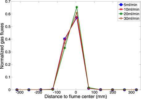
FIGURE 5. Normalized gas fluxes at the top boundary of the domain based on the simulation outcomes.

Bubble Plume Fronts Evolution

The evolution of the plume front was defined by a fixed gas volume fraction, which is equal to 20% of the maximum gas volume fraction. Note that the gas volume fraction is defined within a Representative Elementary Volume (REV) of $8\times 8$ mm², consistent with the REV applied for analyzing the laboratory data by Ma et al. (2015). As shown in Figure 6, H_t is the distance of the plume front from the release point before the bubble breakthrough. The evolution of the plume front over time exhibits an advancing speed that is analogous to 5 and 10 ml/min. The advancing speed also behaved similarly for the gas release rates of 20 and 30 ml/min, but both slightly increased compared with the results for the low gas release rates. Unlike the laboratory results given by Ma et al. (2015), there is no consistent advancing speed among the results for the various gas release rates.

FIGURE 6

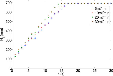
FIGURE 6. Temporal evolution of the bubbles plume fronts under various gas release rates.

The plume breakthrough times were obtained for all cases with different gas release rates by tracking the bubble plume front. In order to test if the numerical results also follow the scaling solutions proposed for the laboratory experiments conditions by Ma et al. (2015), $\ln \left(t\ast \right)$ versus $\ln \left(Q\right)$ was plotted. The slope for the trendline between $\ln \left(t\ast \right)$ and $\ln \left(Q\right)$ is -0.137, which is three times smaller than that of the scaling solution proposed for the laboratory experiment (–0.4) by Ma et al. (2015). The overall $t\ast$ is around 3–5 s smaller than the laboratory results of Ma et al. (2015), as shown in Figure 7.

FIGURE 7

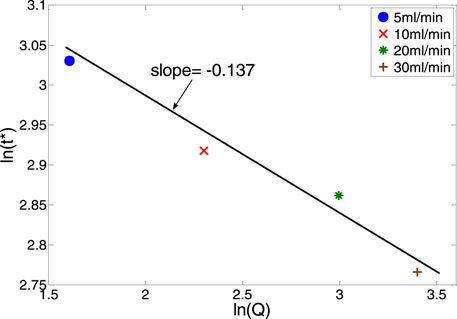
FIGURE 7. Characteristic time $\left(\ln \left(t\ast \right)\right)$ versus gas release rate $\left(\ln \left(Q\right)\right)$.

Bubble Plume Lateral Width Evolution

The mean lateral width of the bubble plume was tracked over time, as shown in Figure 8. The lateral width of the bubble plume gradually increased with the gas release rate. At the initial stage of the plume development (less than 15 s before the bubble plume front breakthrough), the higher gas release rates produced wider plume widths. At the later stage of the plume development, the plume width approached steady-state conditions with time. The temporal variation of the plume width standard deviation exhibited a gradual increase followed by a relatively constant level, especially after the plume breakthrough. Attempts were also given to apply a characteristic width to normalize/non-dimensionalize the numerical results. However, it failed to find a suitable characteristic width to converge all curves into a relatively uniform trend.

FIGURE 8

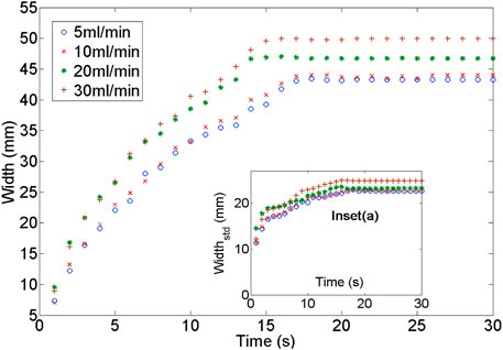
FIGURE 8. The bubble plume lateral width evolution with its standard deviation (inset (a)).

Bubble Plume-Induced Pore Water Movement

The numerical model also demonstrated pore water flows associated with gas ebullition. Circulation was clearly illustrated due to the lift-up of pore water inside the bubble plume and the draw-down of pore water outside the plume. As shown in Figure 9, the vertical pore water flow velocities were plotted along transects at various heights of the simulation domain. Pore water was also descending beside the ascending pore water in the domain centre (more likely within the bubble plume). This descending pore water could be caused by localized circulations inside the plume, which may confine the bubble plume size. Outside the bubble plume, almost all of the water flows downward, and the higher gas release rate leads to a faster pore water velocity.

FIGURE 9

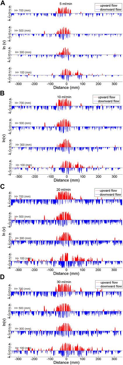
FIGURE 9. The bubble plume-induced pore-water velocity (ln(v)) in the vertical direction under various gas release rates: (A) 5 ml/min; (B) 10 ml/min; (C) 20 ml/min; (D) 30 ml/min. The red lines represent the upward pore water flow, and the blue lines show the downward pore water flow.

The Inconsistency With Prior Experimental Outcomes

The average pore water velocity $\left(v\right)$ over the cross-sectional area outside the bubble plume was plotted versus the gas release rate in Figure 10. Based on the scaling solution described by Ma et al. (2015), $v$ is proportional to $Q^{0.6}$. The numerical results were tested by plotting a trendline with an exponent of 0.6. Unfortunately, the slope of 0.6 underestimated the actual trend, which is better fitted by an incline of 0.8.

FIGURE 10

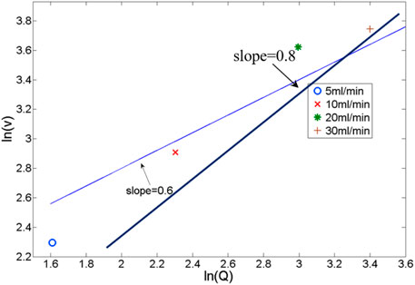
FIGURE 10. Averaged pore water velocity over the cross-sectional area outside the bubble plume.

Compared with laboratory conditions from Ma et al. (2015), the inconsistent modelled results of the bubble plume width and the breakthrough time could be influenced by the drag coefficients $C_d$ applied in the model. A simple numerical experiment was conducted to examine the $C_d$ influence on the bubble plume width. The drag coefficient in Figure 11B is 100 times larger than that of the drag coefficient in Figure 11A. Consequently, the lateral bubble plume width is almost doubled in Figure 11B. As a result, we exert more resistance force on bubbles by applying a more significant drag coefficient. Thus, the vertical velocity of the bubble plume would be reduced, prolonging the bubble plume breakthrough time and enhancing bubble dispersion. Those effects may lead to more realistic results than the laboratory data from Ma et al. (2015). The bubble plume breakthrough time modelled in this work is less than the breakthrough time observed in the laboratory experiments from Ma et al. (2015) by approximately 3–5 s.

FIGURE 11

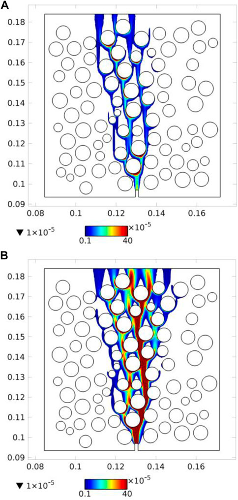
FIGURE 11. The gas volume fraction distributions under two drag coefficients: the $C_d$ in Figure 11 (B) is 100 times larger than the $C_d$ in Figure 11 (A). The round circles are the particles in the domain.

Further investigations are required to better understand the impacts of drag coefficients on the bubble transporting behaviour and ambient pore water flow and develop a proper drag coefficient function to replicate the laboratory experiments. A parametric and sensitivity study might also need to be carried out for those purposes in the future. However, this does not undermine the value of this numerical modelling work as the first attempt because it is still a good initiation in addition to the prior physical modelling.

Conclusion and Reflections

A pore-scale two-phase bubbly flow model was developed and tested in this study. The numerical model was applied to replicate the laboratory experiments and allow more detailed studies, which were not feasible in the laboratory experiments. The preliminary numerical results have revealed that the proposed continuum numerical method can simulate bubbly flow events and bubble-water dynamic interaction phenomena. This numerical model was validated by conserving the gas mass in the simulating domain. The simulation results provide more physical insights into complex bubble transport behaviour in porous media through specific plume parameters. The breakthrough time of the bubble plume and the cross-sectional averaged velocity of ambient pore water flow were manifested to be proportional to the gas release rates in the logarithmic scales. Also, the bubble plume width was also observed to be proportional to the gas release rates. Moreover, the gas distribution on the top boundary could be observed.

This study examined the numerical outcomes against laboratory results and the scaling solution described in our previous experimental works. Although the modelling results do not match the laboratory data quantitatively, the modelled results capture bubble plumes’ trends/tendencies/features under various gas release rates, such as the plume width, plume breakthrough time, and pore water flow velocity.

The proposed numerical method has a relatively high computing cost, with around one million elements needed to represent the domain. This requires approximately 1 week to complete one gas release rate simulation case. As it was demonstrated that the drag coefficient applied in the model impacts the bubble transport behaviour, further studies should be carried out to focus on the drag coefficient effects. In addition, the solid particles packing method should also be investigated further in the future.

Scaling solutions proposed in the prior experimental study may only be applicable for discrete bubble transport in porous media with a specific range of porosity and permeability. Therefore, further studies are required to examine the hydrodynamic interactions between bubble ebullition and pore water under different boundary conditions within different types of porous media. Furthermore, the effects of the water table on microbubble transport behaviour could also be studied.

Bubble transport in the porous media has been studied with a minimal ratio of bubble size to solid particle size without observing bubble trapping. By increasing this ratio, the porous media could trap the bubbles in the pore space or pore throat. This bubble trapping would certainly change bubble transport behaviour and the hydrodynamic interactions between bubbles and ambient pore water. Further studies are required to investigate various ratios between bubbles and solid particle sizes. Thus a bubble phase diagram could be produced to determine the correlation between the bubbles’ trapping and velocity.

Data Availability Statement

The raw data supporting the conclusion of this article will be made available by the authors, without undue reservation.

Author Contributions

Conceptual design: YM and GY; Modelling method: YM; Writing: YM and GY; Editing: GY; Supervision: AS.

Funding

The work was funded by the National Key Research and Development Program of China (2021YFB2601100) and Fundamental Research Funds for DMU 3132022168. This work was also funded by the Linkage Project (LP120100662), Multiscale two-phase flow in complex coal seam systems, funded by the Australian Research Council and supported by a Queensland Science Fellowship awarded to AS.

Conflict of Interest

The authors declare that the research was conducted in the absence of any commercial or financial relationships that could be construed as a potential conflict of interest.

Publisher’s Note

All claims expressed in this article are solely those of the authors and do not necessarily represent those of their affiliated organizations, or those of the publisher, the editors and the reviewers. Any product that may be evaluated in this article, or claim that may be made by its manufacturer, is not guaranteed or endorsed by the publisher.

Acknowledgments

The authors would like to acknowledge support from the Geotechnical Engineering Centre (GEC), School of Civil Engineering, the University of Queensland, Australia.

References

Abreu, L. D. V., and Johnson, P. C. (2005). Effect of Vapor Source−Building Separation and Building Construction on Soil Vapor Intrusion as Studied with a Three-Dimensional Numerical Model. Environ. Sci. Technol. 39 (12), 4550–4561. doi:10.1021/es049781k

PubMed Abstract | CrossRef Full Text | Google Scholar

Annunziatellis, A., Beaubien, S., Bigi, S., Ciotoli, G., Coltella, M., and Lombardi, S. (2008). Gas Migration along Fault Systems and through the Vadose Zone in the Latera Caldera (Central Italy): Implications for CO2 Geological Storage. Int. J. Greenh. Gas Control 2 (3), 353–372. doi:10.1016/j.ijggc.2008.02.003

CrossRef Full Text | Google Scholar

Bear, J. (1972). Dynamics of Fluids in Porous Media. New York, USA: American Elsevier Publishing Company, Inc., Environmental science series.

Google Scholar

Brown, A. (2000). Evaluation of Possible Gas Microseepage Mechanisms. AAPG Bull. 84 (11), 1775–1789. doi:10.1306/8626c389-173b-11d7-8645000102c1865d

CrossRef Full Text | Google Scholar

Chang, K. A., and Lindquist, W. B. (2020). The Dynamics of Gas-Bubble Formation at Saturated Conditions in Porous Media Flow. Sci. Rep. 10 (1), 13175. doi:10.1038/s41598-020-69506-w

PubMed Abstract | CrossRef Full Text | Google Scholar

Charbeneau, R., and Sherif, S. (2002). Groundwater Hydraulics and Pollutant Transport. Appl. Mech. Rev. 55 (2), B38–B39. doi:10.1115/1.1451232

CrossRef Full Text | Google Scholar

Clift, R., Grace, J. R., and Weber, M. E. (2005). Bubbles, Drops, and Particles. USA: Dover Publications.

Google Scholar

Crowe, C., Sommerfeld, M., and Tsuji, Y. (1998). Multiphase Flows with Droplets and Particles. Florida, United States: CRC Press.

Google Scholar

Duddridge, G. A., Grainger, P., and Durrance, E. M. (1991). Fault Detection Using Soil Gas Geochemistry. Q. J. Eng. Geol. Hydrogeology 24 (4), 427–435. doi:10.1144/gsl.qjeg.1991.024.04.09

CrossRef Full Text | Google Scholar

Etiope, G., and Martinelli, G. (2002). Migration of Carrier and Trace Gases in the Geosphere: an Overview. Phys. earth Planet. interiors 129 (3-4), 185–204. doi:10.1016/s0031-9201(01)00292-8

CrossRef Full Text | Google Scholar

Fleischer, R. L., and Mogro-Campero, A. (1978). Mapping of Integrated Radon Emanation for Detection of Long-Distance Migration of Gases within the Earth: Techniques and Principles. J. Geophys. Res. 83 (B7), 3539–3549. doi:10.1029/jb083ib07p03539

CrossRef Full Text | Google Scholar

Fleischer, R. L., and Mogro-Campero, A. (1979). Radon Enhancements in the Earth: Evidence for Intermittent Upflows? Geophys. Res. Lett. 6 (5), 361–364. doi:10.1029/gl006i005p00361

CrossRef Full Text | Google Scholar

Hadamard, J. (1911). Mouvement permanent lent d'une sphere liquid et visqueuse dans un liquide visqueux: CR Hebd. Seances Acad. Sci. Paris 152, 1735–1738.

Google Scholar

Happel, J., and Brenner, H. (1983). Low Reynolds Number Hydrodynamics: With Special Applications to Particulate Media. Dordrecht, Netherlands: Springer Netherlands.

Google Scholar

Kitanidis, P. K. (1997). Introduction to Geostatistics: Applications in Hydrogeology. Cambridge, United Kingdom: Cambridge University Press.

Google Scholar

Kristiansson, K., and Malmqvist, L. (1984). The Depth-Dependence of the Concentration of 86222Rn in Soil Gas Near the Surface and its Implication for Exploration. Geoexploration 22 (1), 17–41. doi:10.1016/0016-7142(84)90003-6

CrossRef Full Text | Google Scholar

Li, Q., Ito, K., Wu, Z., Lowry, C. S., and Loheide II, S. P. (2009). COMSOL Multiphysics: A Novel Approach to Ground Water Modeling. Groundwater 47 (4), 480–487. doi:10.1111/j.1745-6584.2009.00584.x

CrossRef Full Text | Google Scholar

Ma, Y., Kong, X.-Z., Scheuermann, A., Galindo-Torres, S. A., Bringemeier, D., and Li, L. (2015). Microbubble Transport in Water-Saturated Porous Media. Water Resour. Res. 51 (6), 4359–4373. doi:10.1002/2014wr016019

CrossRef Full Text | Google Scholar

Ma, Y. (2015). Preferential Flow Paths in A Complex Coal Seam System [PhD Graduation Thesis. Australia: University of Queensland, 141.

Google Scholar

Ma, Y. (2012). Preferential Flow Paths in a Complex Coal Seam System: Australia. Australia: University of Queensland, 66.

Google Scholar

MacElvain, R. (1969). Mechanics of Gaseous Ascension through a Sedimentary Column: Unconventional Methods in Exploration for Petroleum and Natural Gas. Editor W. B. Heroy. (Dallas, TX, United Kingdom: Southern Methodist University Press), 15–28.

Google Scholar

Mahabadi, N., Zheng, X., Yun, T. S., van Paassen, L., and Jang, J. (2018). Gas Bubble Migration and Trapping in Porous Media: Pore-Scale Simulation. J. Geophys. Res. Solid Earth 123 (2), 1060–1071. doi:10.1002/2017jb015331

CrossRef Full Text | Google Scholar

Mualem, Y. (1976). A New Model for Predicting the Hydraulic Conductivity of Unsaturated Porous Media. Water Resour. Res. 12 (3), 513–522. doi:10.1029/wr012i003p00513

CrossRef Full Text | Google Scholar

Price, L. C. (1986). A Critical Overview and Proposed Working Model of Surface Geochemical Exploration: Unconventional Methods in Exploration for Petroleum and Natural Gas IV. Editor M. J. Davidson. (Dallas, TX, United Kingdom: Southern Methodist University Press), 245–309.

Google Scholar

Rybczynski, W. (1911). Uber die fortschreitende Bewegung einer flussigen Kugel in einem zahen Medium. Bull. Acad. Sci. Crac. A 1, 40–46.

Google Scholar

Saunders, D. F., Burson, K. R., and Thompson, C. K. (1999). Model for Hydrocarbon Microseepage and Related Near-Surface Alterations. AAPG Bull. 83 (1), 170–185. doi:10.1306/00aa9a34-1730-11d7-8645000102c1865d

CrossRef Full Text | Google Scholar

To, H. D., Galindo-Torres, S. A., and Scheuermann, A. (2016). Sequential Sphere Packing by Trilateration Equations. Granul. Matter 18 (3), 1–14. doi:10.1007/s10035-016-0666-5

CrossRef Full Text | Google Scholar

Vakarelski, I. U., Manica, R., Tang, X., O’Shea, S. J., Stevens, G. W., Grieser, F., et al. (2010). Dynamic Interactions between Microbubbles in Water. Proc. Natl. Acad. Sci. U.S.A. 107 (25), 11177–11182. doi:10.1073/pnas.1005937107

PubMed Abstract | CrossRef Full Text | Google Scholar

Van Genuchten, M. T. (1980). A Closed-form Equation for Predicting the Hydraulic Conductivity of Unsaturated Soils. Soil Sci. Soc. Am. J. 44 (5), 892–898. doi:10.2136/sssaj1980.03615995004400050002x

CrossRef Full Text | Google Scholar

Várhegyi, A., Baranyi, I., and Somogyi, G. (1986). A Model for the Vertical Subsurface Radon Transport in “Geogas” Microbubbles. Geophys. Trans. 32 (3), 235–253.

Google Scholar

Wan, J., Veerapaneni, S., Gadelle, F., and Tokunaga, T. K. (2001). Generation of Stable Microbubbles and Their Transport through Porous Media. Water Resour. Res. 37 (5), 1173–1182. doi:10.1029/2000wr900331

CrossRef Full Text | Google Scholar

Yan, G., Bore, T., Bhuyan, H., Schlaeger, S., and Scheuermann, A. (2022a). The Technical Challenges for Applying Unsaturated Soil Sensors to Conduct Laboratory-Scale Seepage Experiments. Sensors 22 (10), 3724. doi:10.3390/s22103724

PubMed Abstract | CrossRef Full Text | Google Scholar

Yan, G., Bore, T., Li, Z., Schlaeger, S., Scheuermann, A., and Li, L. (2021a). Application of Spatial Time Domain Reflectometry for Investigating Moisture Content Dynamics in Unsaturated Loamy Sand for Gravitational Drainage. Appl. Sci. 11 (7), 2994. doi:10.3390/app11072994

CrossRef Full Text | Google Scholar

Yan, G., Li, Z., Bore, T., Galindo Torres, S. A., Scheuermann, A., and Li, L. (2022b). A Lattice Boltzmann Exploration of Two-phase Displacement in 2D Porous Media under Various Pressure Boundary Conditions. J. Rock Mech. Geotechnical Eng.. doi:10.1016/j.jrmge.2022.05.003

CrossRef Full Text | Google Scholar

Yan, G., Li, Z., Bore, T., Torres, S. A. G., Scheuermann, A., and Li, L. (2021b). Discovery of Dynamic Two-phase Flow in Porous Media Using Two-Dimensional Multiphase Lattice Boltzmann Simulation. Energies 14 (13), 4044. doi:10.3390/en14134044

CrossRef Full Text | Google Scholar

Yan, G., Li, Z., Galindo Torres, S. A., Scheuermann, A., and Li, L. (2022c). Transient Two-phase Flow in Porous Media: A Literature Review and Engineering Application in Geotechnics. Geotechnics 2 (1), 32–90. doi:10.3390/geotechnics2010003

CrossRef Full Text | Google Scholar

Yan, G., Ma, Y., Scheuermann, A., and Li, L. (2022d). The Hydraulic Properties of Aquabeads Considering Forchheimer Flow and Local Heterogeneity. Geotechnical Test. J. 45, 4. doi:10.1520/gtj20210234

CrossRef Full Text | Google Scholar

Yi, T., Yang, G., Wang, B., Zhuan, R., Huang, Y., and Wu, J. (2022). Dynamics of a Gas Bubble Penetrating through Porous Media. Phys. Fluids 34 (1), 012103. doi:10.1063/5.0076298

CrossRef Full Text | Google Scholar

You, K., Zhan, H., and Li, J. (2011). Gas Flow to a Barometric Pumping Well in a Multilayer Unsaturated Zone. Water Resour. Res. 47–5. doi:10.1029/2010wr009411

CrossRef Full Text | Google Scholar