 Zhenghong Song
 Xiangfang Zeng
 Benxin Chi
 Feng Bao1
 Abayomi Gaius Osotuyi
- 1State Key Laboratory of Geodesy and Earth’s Dynamics, Innovation Academy for Precision Measurement Science and Technology, Chinese Academy of Sciences, Wuhan, China
- 2School of Earth and Space Sciences, University of Science and Technology of China, Hefei, China
Distributed acoustic sensing (DAS) is a novel seismological observation technology based on the fiber-optic sensing method, and can transform existing urban fiber-optic cables into ultra-dense array for urban seismological researches, thus opening abundant opportunities for resolving fine details of near surface structures. While high frequency ambient noise recorded on DAS has been applied in surface wave tomography, it is often difficult to extract a clear dispersion curve for the data recorded by urban internet cable because of the effect of precursor signals on noise correlation functions due to uneven distribution of noise sources, and weak coupling between the cable and the solid earth. In this study, we investigate the performance of the three-station interferometry method for improving the noise cross-correlation functions of the linear array. We applied this method to a DAS dataset acquired in an urban area, suppressed the precursor signal, improved the measurement of the dispersion curve, and constructed a 2D S-wave profile that reveals the hidden fault beneath the city. We also observed that the convergence of noise cross-correlation functions with weak coupling was significantly accelerated using this method. We employed this method to improve the signal quality of surface waves at far offset for the long segment, thus obtaining a more accurate dispersion curve. In conclusion, the three-station interferometry is an effective method to enhance the surface wave signal and suppress the precursor signal retrieved from the data recorded by urban internet cable, which could help in providing high resolution images of shallow structures in built-up areas.
Introduction
High-resolution imaging of subsurface structures plays an important role in urban construction planning (e.g., underground space utilization, (Bobylev, 2010)), and geological disaster prevention (e.g., sinkhole detection (Cueto et al., 2018) and earthquake intensity estimation (Chen et al., 2009)). The seismic method is an effective tool to achieve high-precision subsurface imaging by analyzing the seismic wave signals generated from controlled active sources or natural sources. Subsurface anomalies can be identified using active sources with high signal-to-noise ratio (SNR) ratio and desirable observation system (Zandomeneghi et al., 2013). At the same time, reliable results have also been achieved using passive source imaging from ambient noise which is due to human activity (e.g., Lin et al., 2013; Zeng et al., 2021; Mi et al., 2022). Moreover, thickness and shear velocity structure in the top dozens of meters beneath permanent seismic stations have been resolved from modeling converted high frequency seismic phases from local earthquakes (Li et al., 2014; Ni et al., 2014), and their studies demonstrate a few times of ground motion amplification due to near surface low shear velocity structures. Obtaining a high-resolution subsurface structure relies on short seismic wavelength requiring denser observations, which is a huge challenge in seismic data acquisitions using traditional seismometers. Distributed acoustic sensing (DAS) is a recently developed novel seismic observation system, which measures the seismic signals by analyzing the phase shift of the backscattered pulse in the optical fiber (Zhan, 2020). It is noteworthy to mention that DAS can easily be incorporated with existing urban fiber-optic cables, thereby turning the fiber-optic networks into dense seismographic networks with meter-scale spacing (Parker et al., 2014). DAS has found broad applications and has demonstrated to be a valuable tool in seismological studies such as in signal detection (e.g., Lindsey et al., 2017; Zhu and Stensrud 2019; Wang et al., 2020) and near-surface characterization (e.g., Ajo-Franklin et al., 2019; Spica et al., 2020).
Ambient noise tomography, widely used for urban subsurface structure detection, is achieved via calculating the cross-correlation of continuous ambient noise records (noise cross-correlation function, NCF) and stacking them to extract surface wave signals for inversion (Bensen et al., 2007). However, the precursor signals produced by heterogeneous noise distribution in urban areas seriously affect the quality of NCF and the results of ambient noise tomography (Galetti and Curtis, 2012; Retailleau and Beroza 2021). The noise excited by vehicles traveling along the fiber-optic cable is contributive, while the noise generated by vehicles across the cable and persistent localized human activities are adverse for ambient noise tomography (Song et al., 2021). Furthermore, the urban existing fiber-optic cables are packaged with different structures and deployed in a variety of ways, so the transfer function of the coupling is influenced by many factors and needed to be further studied (e.g., Lindsey et al., 2020b). We assumed that the coupling of the fiber-optic cables lying in the same polyvinyl chloride pipe is uniform but the coupling of pipeline to soil is various and the changes in phase response are ignorable. As a result of weak coupling, the amplitude response is low, which decreases the SNR of effective noise signals, and it would require a longer time span stacking to obtain a stable NCF (Lin et al., 2021). However, long-time span stacking may not obtain the correct NCF when the traffic signal is too weak to exceed the instrument’s self-noise level.
Therefore, it is necessary to enhance the surface wave and suppress the precursor signals for the NCF. Stehly et al. (2008) reconstructed the surface wave signal between two stations by calculating the cross-correlation of the coda waves of the NCF between the stations with a third station (C3). Froment et al. (2011) demonstrated that C3 can well suppress the effects caused by distributions of non-isotropic sources by analyzing 150 continuously recording stations. Curtis and Halliday (2010) proposed three-station interferometry for direct wave (TSI), which used the entire NCF rather than the coda wave of the NCF. The convolution of the entire NCFs was calculated when the third station lies between the two stations, while the cross-correlation was calculated when the third station is located outside the two stations. Zhang et al., (2020a) compared the surface wave signals extracted from C3 and TSI, and suggested there are small biases in the dispersion curve. The biases arise from the geometry of the stations, which assumes the distance difference equal to 0 (distance difference is the difference between the distance of two stations and the sum/difference of the distances from the third station to the two stations when the third station lie in/out the two stations). The influence of distance difference might be negligible for a nearly straight linear array (Lin et al., 2008). Qiu et al. (2021) successfully enhanced the surface wave signals extracted from the NCF of a linear array using the TSI method, thereby making the method potentially applicable to improve ambient noise tomography results for urban linear DAS array.
In this study, we adopted the TSI method on a real-world DAS dataset and analyzed its improvement in ambient noise tomography. First, we showed a set of NCFs retrieved from the data recorded by urban internet cable in a built-up area and estimated the noise intensity and distribution around the fiber-optic cable. Then, we introduced the TSI method and used this method to denoise the precursor signals. The surface wave signals were enhanced significantly, and clear dispersion curves can be obtained to construct the subsurface structure. Finally, we demonstrate that the TSI method can effectively improve the temporal and spatial resolution of ambient noise tomography by discussing the coupling and length of the segment.
Data and methods
The experiment was carried out in Binchuan county, Yunnan Province, southwest of China (Figure 1). A 5.2 km long internet fiber-optic cable lying in a polyvinyl chloride (PVC) pipe, which was buried at about 30 cm beneath two streets (Taihe Road and Jinniu Road, Wang et al., 2021a), was used in the experiment. The Helios Theta DAS Interrogator was connected to one end of the fiber-optic cable, with a spacing of 7.5 m (gauge length is set at 10.9 m), for 16-h continuous strain data acquisition. A previous study suggested that the noise source in the Taihe Road is distributed along the fiber-optic cable, which benefits for imaging, and the 2D S wave velocity profile has been constructed to reveal the low velocity zone along the road (Song et al., 2021). However, it is difficult to obtain clear dispersion curves along the Jinniu Road for ambient noise tomography, and we suspect this is due to the heterogeneous distribution of noise.
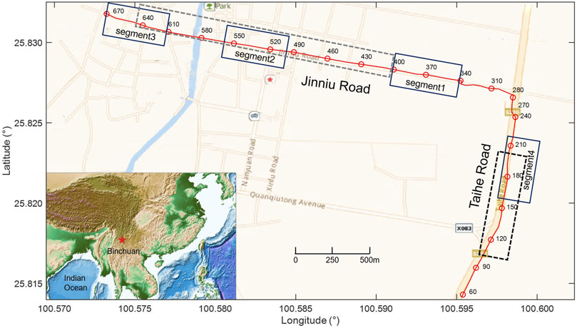
FIGURE 1. The location of the experiment. The red line is fiber-optic cable, which is distributed along two streets (Taihe Road and Jinniu Road). The numbers around the red circles are the channel indexes. The segments framed by the solid and dashed lines are used for analysis in the later section.
For instance, we choose three segments along the Jinniu Road for our analysis (segment 1, CH340-400, segment 2, CH500-560, and segment 3, CH610-670, in Figure 1). The first channel of each segment was used as the virtual source, and the other channels were virtual receivers to calculate the NCF. Song et al. (2021) suggested that the frequency range of ambient noise is 1–30 Hz and a stable NCF can be obtained with 4-h ambient noise data during the daytime. Therefore, for every channel, we resampled a 4-h continuous dataset from 500 to 100 Hz to reduce computing time and bandpass filtered it into 1–30 Hz. The dataset was cut into 30 s time windows, and normalized in time and frequency domains. Then, we calculated the cross-correlation function for each window of the virtual source and virtual receiver. The final NCF was obtained by stacking all the cross-correlation functions. The combination of the NCFs of all the virtual receivers and the virtual source is a common virtual-shot gather. Figures 2A–C are the common virtual-shot gathers of the previous three segments. For segment 1, the surface wave appears in the negative lag of the NCFs, indicating that the noise mainly comes from the direction of Taihe Road. However, the precursor seismic phases appear before the direct surface wave for segments 2 and 3 (Figure 2), and it is produced by complex traffic activities. We stacked the positive and negative lags to reduce the effects of the asymmetric noise source distribution and employed the multi-channel analysis of the surface wave method (MASW, Park et al., 1999) to extract the corresponding dispersion curve (Figures 2D–F). A low frequency (1–5 Hz) dispersion curve was achieved for segment 1, but it is difficult to obtain a continuous dispersion curve for segments 2 and 3.
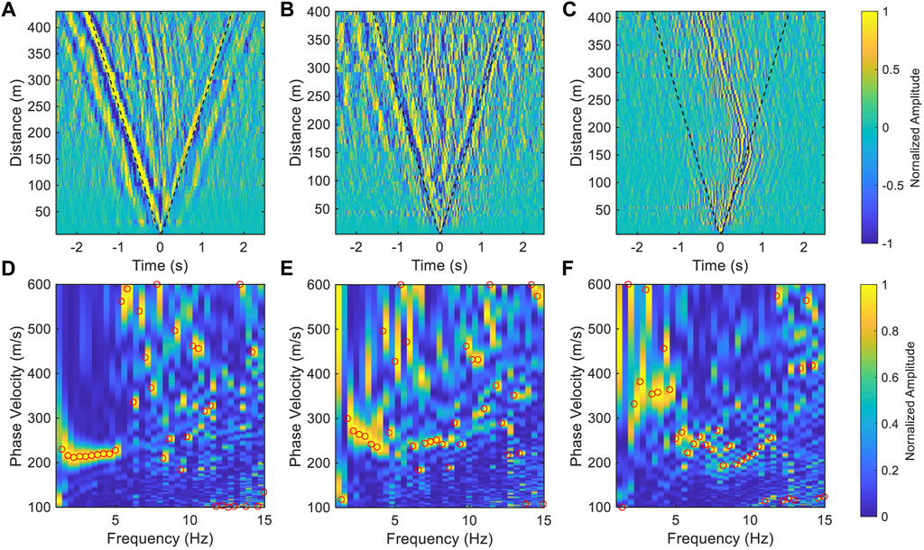
FIGURE 2. The example of common virtual-shot gathers and the dispersion spectra. (A–C) are the NCF waveform for segments 1, 2, and 3 in Figure 1, respectively. The black dashed lines in (A–C) represent a velocity of 250 m/s. (D–F) are the dispersion spectra of the three segments, respectively. The red circles indicate the maximum energy at each frequency.
To analyze the generation of the precursor signals, we estimated the noise intensity distribution around the fiber-optic cables by the back projection method (e.g., Li et al., 2020; Rabade et al., 2022). To estimate the noise intensity, we establish a 600 by 600 m2 area where we set up the location of the virtual source as the origin and the direction of the cable as the y-axis. For any particular location within this area, the difference between the distance from such location to the virtual source and the virtual receiver was calculated. The difference in arrival time was obtained according to the velocity of the surface wave (about 250 m/s, Figure 2). We used a 0.2 s time window centered around the time shift in the NCF (time shift equals the value of arrival time difference), and subsequently calculated the root mean square of the waveform within the time window. The noise intensity of this particular location was obtained by the summation of all the root mean squares of the common virtual-shot gather. The ambient noise intensity distribution was derived by calculating all the locations in this area, and the results are shown in Figure 3. As mentioned earlier, the noises of segment 1 are concentrated in the direction of Taihe road. The noise intensity on the left and right sides of the fiber-optic cables cannot be distinguished because of the linear array. The noise around segment 2 comes from different directions controlled by multiple location noise sources, especially, near the two crossings (Figure 3). In contrast, the noise of segment 3 is dominated by the persistent localized noise source in the array.
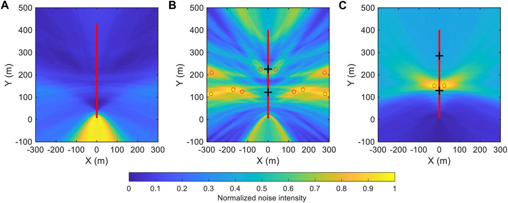
FIGURE 3. The ambient noise intensity around the fiber-optic cable. (A–C) are the noise intensity of segment 1, 2, and 3, respectively in Figure 1. The red lines indicate the fiber-optic cable. The black crosses in (B,C) are the road intersections, while the red circles are the local maxima of noise intensity.
To suppress the precursor seismic phases and enhance the surface waves, the TSI method was employed in this study. Figure 4 is a simplified schematic showing the processing flow as follows: First, for the two channels (Si and Sj) whose NCF is to be enhanced, a third channel (Sk) was selected to calculate the NCFs with these two channels, respectively. Then, we stacked the positive and negative lags and computed the convolution of the two NCFs to obtain the interferometry waveform if Sk lies between Si and Sj (inner-source zone), otherwise, we computed the cross-correlation (outer-source zone) (Eq. 1). The denoised NCF of the two stations (Si and Sj) is obtained by looping all third channels and stacking the interferometry waveforms (Eq. 2). We arrived at the enhanced NCF between all stations by changing the channels of Si and Sj, and by this, an iteration is completed. The same cycle is repeated until a stable result is achieved. It is worth noting that there is a pi/4 phase shift between the calculated NCF and true NCF when the source and receiver are linearly distributed (Halliday and Curtis, 2008; Lin et al., 2008; Qiu et al., 2021). The MASW method, however, measures the phase difference of the multi-channel surface wave signals to determine the phase velocity dispersion curve, so the effect of the pi/4 phase difference could be eliminated.
where the
where the
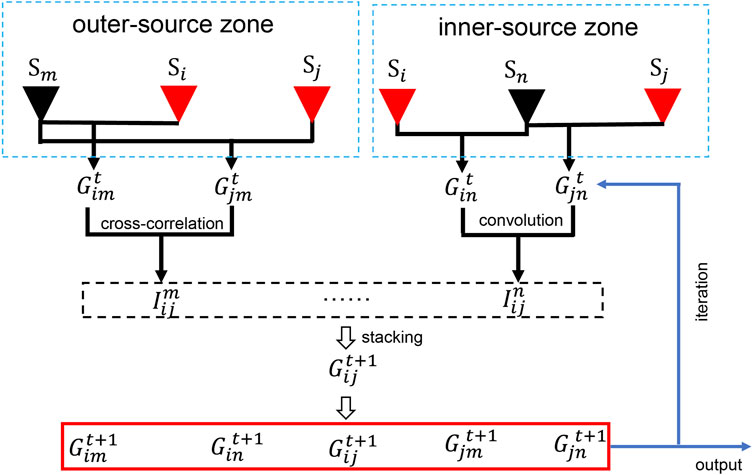
FIGURE 4. Sketch of the TSI method. The red triangles (Si and Sj) indicate the channel pair whose NCF is to be enhanced, and the black triangles are the third channel.
Results
Figure 5A shows the variation of the iterated waveforms of a common virtual-shot gather, when the virtual source is located at CH630. The raw NCF waveforms were tapered within a range of 100–800 m/s to decrease the unwanted body waves or noise signals. The signals at far offset were enhanced significantly and the surface waves dominated in the NCFs after 2 iterations. The improvement becomes little after several iterations and the signals converge to a stable result. The SNR, which is defined as the ratio of the maximum amplitude of the signal windows and the root mean square of the noise windows, increases up to 6 as the iteration increases (Figure 5A). The L1-norm of the difference in the model update is as low as 0.3% while the average of the correlation coefficient before and after model update of all virtual-shot gathers is up to 99.7% after 5 iterations (Figure 5B). The denoised waveforms of the three segments are shown in Figure 6. For segment 1, even if it is not affected by the noise source distribution, the random noise in the NCF was suppressed significantly. The surface wave in high frequency was improved and the frequency band of the dispersion curve was also extended to provide a higher resolution of shallow structure. For the other segments, the precursor seismic phases were removed and the surface waves were enhanced. The 1–10 Hz clear Rayleigh wave phase velocity dispersion curve was extracted to construct the S-wave velocity structure.
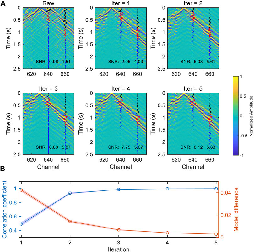
FIGURE 5. (A) The variation of the waveform of segment 3 with the iteration using the TSI method. The virtual source is located at CH630. The blue lines are the waveforms of CH640 and CH660, the black and red lines represent noise and signal windows, respectively. (B) The variation of model correlation coefficient and model difference with iteration. The blue and red shading represent 95% confidence intervals for the correlation coefficient and model difference, respectively.
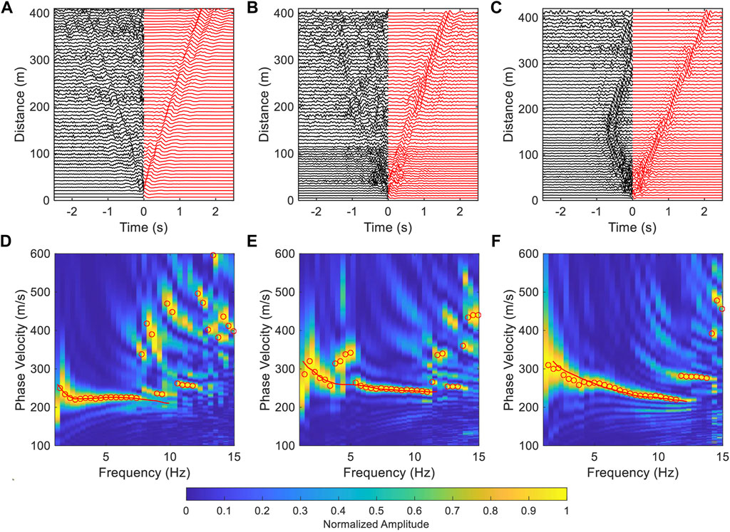
FIGURE 6. The waveform and dispersion spectra after the TSI method. (A–C) are the waveforms of segment 1, 2, and 3, respectively. The black lines are the symmetric to the positive lag of the raw NCFs while the red lines are the denoised NCFs. (D–F) are the dispersion spectra of the denoised waveforms of (A–C), respectively. In (D–F), the red circles represent the maximum energy at each frequency and the red lines are the picked dispersion curves.
The TSI method was utilized to enhance the surface wave along the Jinniu Road for ambient noise tomography. The array was divided into 70 segments and each segment consists of 40 channels (about 300 m) while the overlap between two consecutive segments is 35-channel long (about 262.5 m). 70 dispersion curves were extracted for 1D substructure inversion after the calculation and reconstruction of the surface wave. Typically, the maximum inversion depth is less than half of the maximum wavelength (Song et al., 2021), and in this study, the maximum wavelength is about 300 m according to the dispersion curve (Figure 6), which reveals the top 100 m subsurface structure. For the inversion, the model consists of five layers, including two 20-m layers, two 30-m layers, and a half space. Due to the lack of accurate P-wave velocity structure for this region and that the surface wave dispersion curve is not very sensitive to the P-wave velocity structure and density (Song et al., 2018), the P-wave velocity and density were determined by an empirical relationship (Brocher, 2005, Equation (3) and (4), and only the S-wave velocity was inverted.
where the Vp and Vs are the P-wave and S-wave velocity, respectively.
The neighborhood algorithm (Sambridge 1999), a global search method was utilized for the inversion, and the forward modeling of the dispersion curve was conducted with the Computer Programs for Seismology (Herrmann 2013). The 2D profile beneath the Jinniu Road was obtained by assembling all 1D models (Figure 7A). The shallow structure (<20 m) along the Jinniu Road is homogeneous, indicating the sediment coverage is evenly distributed in the shallow layer. But, the deep structure (>20 m) changes greatly in the lateral direction, and the velocity on the east side is lower, which is consistent with the result of Taihe Road (Song et al., 2021). The dispersion curves fitted well (Figures 7B–E) and suggested that the phase velocity at low frequency on the east side is lower than that on the west side. The north-south trending mountains on both sides of the Binchuan county cause significant velocity differences in the east-west direction. Zhang et al., 2020b suggested that there may be a hidden fault in the west of the county, which is consistent with our results. This result indicated that the combination of urban internet fiber-optic cables with DAS technology, using the TSI method for ambient noise tomography, is highly plausible for achieving ultra-high-density observations, which can be used to produce high-precision images of urban subsurface structures.
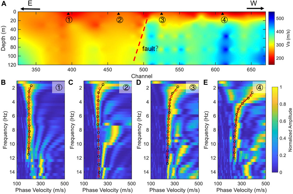
FIGURE 7. (A) The S-wave structure beneath the Jinniu Road. (B–E) are the dispersion curves fitting, corresponding to the positions of the four triangles in (A). The black lines and red lines indicate the observed dispersion curves and the theoretical dispersion curves predicted by the inverted models, respectively.
Discussion
In addition to the distribution of ambient noise, the coupling of the fiber-optic cables is also an important factor that influence ambient noise tomography in urban areas. Most of the urban fiber-optic cables are laid in the PVC pipe, and some parts are directly buried in the soil or hung in the air. It often takes stacking of data acquired over a long time span to obtain a clear surface wave signal on the NCF because of the weak coupling between the cable in the casing pipe and the solid earth (Lin et al., 2021), which decreases the temporal resolution of ambient noise tomography. Furthermore, we discussed the effect of the TSI method on the enhancement of the coherence surface wave signals in the case of weak coupling. The ambient noise in the vicinity of Taihe Road is distributed along the fiber-optic cable, and the clear surface wave signals emerged on the NCF for a 4-h data (Song et al., 2021). Assuming that the responses of all channels are the same, weak coupling reduces the SNR of the NCF for the same time span stacking. We selected a section of the fiber-optic cable (CH160-210, segment 4 in Figure 1), and used the NCF calculated with 4-h and 30-s data to simulate the results of good and weak coupling for the same time span stacking, respectively. The coherent surface wave signals cannot be seen for the weak coupling, and a continuous and accurate dispersion curve cannot be obtained (Figures 8A,D). We used the TSI method to further process the 30-s NCF result, and the surface wave signal was enhanced significantly (Figure 8C). The dispersion curve of the 30-s NCF was observed to be consistent with the results obtained from the 4-h data (Figures 8E,F). This result indicated that the TSI method is suitable for an imperfectly coupled cable setup and can improve the temporal resolution of ambient noise tomography by accelerating the convergence of the NCF.
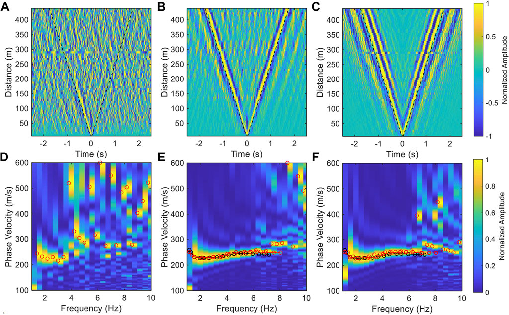
FIGURE 8. Speed-up convergence of NCF via the TSI. (A,B) are the common virtual-shot gather of segment 4 calculated with 30-s and 4-h data, respectively. (C) is the denoised result of (A), and the negative lag of (C) is symmetric to its positive lag. The black dashed lines represent a velocity of 250 m/s. (D–F) are the dispersion spectra of (A–C), respectively. The red and black lines are the picked dispersion curves of (E,F), respectively.
Forbriger et al. (2003) demonstrated that the resolution of the dispersion spectrum is related to the frequency and the length of the segment used for MASW (Eq. 5). That is, with a fixed length segment, the resolution of high frequency is significantly higher than that of low frequency, which has been demonstrated in the previous results (Figure 6). Therefore, increasing the length of the segment is beneficial to improving the accuracy of the dispersion curve in the low frequency range. However, due to the effect of coupling and ambient noise attenuation, the SNR at far offset is low in the real data (CH100-200, ∼750 m, black dashed box in Figure 1), which limits the extraction of the dispersion curve (Figure 9). We processed this dataset with the TSI method and successfully enhanced the surface wave signal at far offset (Figure 9D). The uncertainty of the dispersion curve decreases significantly as the length of the segment increases (Figures 9E,F). Due to MASW measures the average dispersion curve of the segment, there is a tradeoff between the lateral resolution of subsurface structure and the resolution of dispersion spectrum. We can use the long segment combined with the TSI method to obtain a dispersion curve that provides a reference for the short segments. Thereby, this improves the accuracy of dispersion curve extraction without reducing the spatial resolution.
where d represents the relative value of resolution in the dispersion curve, which is expressed as the width of 90% maximum energy of the dispersion spectrum in this paper; f is the frequency and L is the length of the segment.
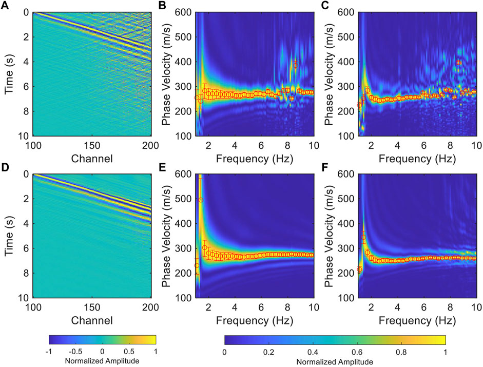
FIGURE 9. The improvement of the resolution of dispersion spectra of the long segment with the TSI method. (A) The NCFs of a long segment (black dashed box in Figure 1). (B) The dispersion spectrum is calculated using the waveforms of CH100-150, the red bars are the picked uncertainties which is defined as the zone with 90% of the maximum energy of each frequency. (C) is same as (B) but for CH100-200. (D–F) same as (A–C) but for the denoised waveforms using the TSI method.
The dispersion curve extracted by the MASW method represents the average velocity beneath the investigated segment, hence, the dispersion curve cannot be obtained when there are significant variations in the subsurface structure. However, surface wave signals with high signal-to-noise ratio are useful for other seismological imaging methods such as full waveform inversion (e.g., Liu et al., 2017). The imaging result of the short segments shows that there are obvious differences in the subsurface structure beneath the Jinniu Road (Figure 7A), at the same time, the SNR of the surface wave is also lower than that in the Taihe Road (Figure 10A). Furthermore, we selected a long segment in the Jinniu Road (CH400-650, ∼1875 m, gray dashed box in Figure 1) to establish whether the TSI method is effective in the case of uneven subsurface structure. We observed a significant improvement on the raw data, revealing that the surface wave signals at the far offset are well reconstructed via the TSI method (Figure 10B). Because the velocity on the east side of the profile (channel index < CH500) is lower than that on the west side (channel index > CH500), we calculated the dispersion curve for the waveform of the sub-segments. Between CH400-500 (sub-segment i in Figure 10B) and CH500-600 (sub-segment ii in Figure 10B), we arrived at the respective corresponding dispersion curves shown in Figures 10C,D. The relative magnitude of the phase velocity is consistent with the previous result (Figure 7A). To verify the reliability of the results, we first separated CH400-500 and CH500-600 into different segments and thereafter utilized the TSI method to process each of the segments, individually, and extracted their dispersion curves (Figures 10E–H). The dispersion curves are very close to the previous results in Figures 10C,D, thus indicating that the TSI method is effective in resolving the uneven subsurface structure below the array.
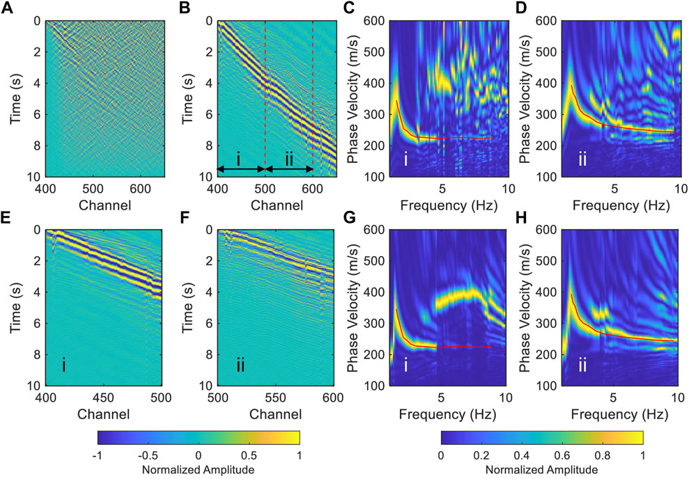
FIGURE 10. The feasibility test of the TSI method in the heterogeneous subsurface structure. (A) The raw common virtual-shot gather of the long segment (gray dashed box in Figure 1). (B) The NCFs after the TSI method. The red dashed lines divided the long segment into sub-segments i (CH400-500) and ii (CH500-600) for dispersion curve calculation. (C,D) are the dispersion spectra of the sub-segment (i) and (ii) cut from (B). (E,F) are the denoised waveforms of the segments of (i) and (ii), respectively. (G) and (H) are the dispersion spectra of (E,F), respectively. The red lines in (C,G) are the dispersion curves extracted from (C), while the red lines in (D,H) are the dispersion curves extracted from (D).
We successfully suppressed the influence of the noise source distribution on ambient noise tomography using the TSI method. However, the characteristics of noise sources are also a common concern in seismological research (e.g., McNamara and Buland, 2004; Retailleau and Beroza, 2021; Song et al., 2021). Determining the properties and distribution of noise sources enables non-intrusive monitoring of human activities and helps to understand the signals that emerge on the NCF. In the past, researchers have analyzed traffic signals recorded by the urban internet cables in application to traffic flow monitoring (e.g., Martin et al., 2018; Lindsey et al., 2020a; Wang et al., 2021b) and vehicle classification (e.g., Liu et al., 2019). High resolution subsurface structures can now better serve in the study of noise sources. Also, an inversion of the distribution of noise sources and the shallow structure can be conducted at the same time (Lehujeur et al., 2016).
Conclusion
In this study, we analyzed the ambient noise data recorded by an urban internet fiber-optic cable. The estimation of the noise intensity near the fiber-optic cable indicates significant influence from crossing traffic. Affected by the uneven noise source distribution and imperfect coupling, it is difficult to extract clear surface wave dispersion for conventional ambient noise tomography with inter-station correlation. We adopted the TSI method to this dataset and successfully suppressed the precursor seismic phases, enhanced the surface wave signals leading to better measurement of dispersion, constructed the shallow shear velocity structure, and revealed a hidden fault. Furthermore, we demonstrated that the TSI method is effective for imperfect coupling, and substantially improved the convergence of the NCF, which enhanced the temporal resolution of ambient noise tomography. For a long segment, the SNR of surface wave signals at far offset is weak due to the effect of coupling and ambient noise attenuation, which limits the accuracy of the dispersion curve extraction. The TSI method can enhance the surface wave signal at the far offset, even though there are significant differences in the subsurface structure. The TSI can improve the ambient noise tomography to construct high resolution structure, which in turn can be used for the study of noise source intensity and distribution, as well as a better understanding of the effect of the noise source distribution on the NCF. In conclusion, the TSI method is an effective method to suppress the effects of uneven noise distribution and enhance the surface wave. Using existing fiber-optic cable in combination with the TSI method for urban ambient noise tomography can produce high-resolution imaging, thus providing helpful information on subsurface structures for civil engineering construction and disaster prevention.
Data availability statement
The raw data supporting the conclusion of this article will be made available by the authors, without undue reservation.
Author contributions
ZS carried out the data processing and wrote the manuscript. XZ led the project design and supervised the data analysis. BC advised on method and commented on the manuscript. FB acquired the data. AO edited the manuscript.
Funding
National Key R&D Program of China (2021YFA0716802), National Natural Science Foundation of China (41974067).
Conflict of interest
The authors declare that the research was conducted in the absence of any commercial or financial relationships that could be construed as a potential conflict of interest.
Publisher’s note
All claims expressed in this article are solely those of the authors and do not necessarily represent those of their affiliated organizations, or those of the publisher, the editors and the reviewers. Any product that may be evaluated in this article, or claim that may be made by its manufacturer, is not guaranteed or endorsed by the publisher.
References
Ajo-Franklin, J. B., Dou, S., Lindsey, N. J., Monga, I., Tracy, C., Robertson, M., et al. (2019). Distributed acoustic sensing using dark fiber for near-surface characterization and broadband seismic event detection. Sci. Rep. 9 (1), 1328. doi:10.1038/s41598-018-36675-8
Bensen, G. D., Ritzwoller, M. H., Barmin, M. P., Levshin, A. L., Lin, F., Moschetti, M. P., et al. (2007). Processing seismic ambient noise data to obtain reliable broad-band surface wave dispersion measurements. Geophys. J. Int. 169 (3), 1239–1260. doi:10.1111/j.1365-246x.2007.03374.x
Bobylev, N. (2010). Underground space in the Alexanderplatz area, Berlin: Research into the quantification of urban underground space use. Tunn. Undergr. Space Technol. 25 (5), 495–507. doi:10.1016/j.tust.2010.02.013
Brocher, T. M. (2005). Empirical relations between elastic wavespeeds and density in the Earth's crust. Bull. Seismol. Soc. Am. 95 (6), 2081–2092. doi:10.1785/0120050077
Chen, Q., Liu, L., Wang, W., and Rohrbach, E. (2009). Site effects on earthquake ground motion based on microtremor measurements for metropolitan Beijing. Sci. Bull. (Beijing). 54 (2), 280–287. doi:10.1007/s11434-008-0422-2
Cueto, M., Olona, J., Fernández‐Viejo, G., Pando, L., and López-Fernández, C. (2018). Karst‐induced sinkhole detection using an integrated geophysical survey: A case study along the riyadh metro line 3 (Saudi arabia). Near Surf. Geophys. 16 (3), 270–281. doi:10.3997/1873-0604.2018003
Curtis, A., and Halliday, D. (2010). Source-receiver wave field interferometry. Phys. Rev. E 81 (4), 046601. doi:10.1103/physreve.81.046601
Froment, B., Campillo, M., and Roux, P. (2011). Reconstructing the Green's function through iteration of correlations. Comptes Rendus Geosci. 343 (8-9), 623–632. doi:10.1016/j.crte.2011.03.001
Forbriger, T. (2003). Inversion of shallow-seismic wavefields: I. Wavefield transformation. Geophysical Journal International 153 (3), 719–734. doi:10.1046/j.1365-246X.2003.01929.x
Galetti, E., and Curtis, A. (2012). Generalised receiver functions and seismic interferometry. Tectonophysics 532, 1–26. doi:10.1016/j.tecto.2011.12.004
Halliday, D., and Curtis, A. (2008). Seismic interferometry, surface waves and source distribution. Geophys. J. Int. 175 (3), 1067–1087. doi:10.1111/j.1365-246x.2008.03918.x
Herrmann, R. B. (2013). Computer programs in seismology: An evolving tool for instruction and research. Seismol. Res. Lett. 84 (6), 1081–1088. doi:10.1785/0220110096
Lehujeur, M., Vergne, J., Maggi, A., and Schmittbuhl, J. (2016). Ambient noise tomography with non-uniform noise sources and low aperture networks: Case study of deep geothermal reservoirs in northern alsace, France. Geophys. J. Int. 208 (1), 193–210. doi:10.1093/gji/ggw373
Li, Z., Ni, S., and Somerville, P. (2014). Resolving shallow shear‐wave velocity structure beneath station CBN by waveform modeling of the M w 5.8 Mineral, Virginia, earthquake sequence. Bull. Seismol. Soc. Am. 104 (2), 944–952. doi:10.1785/0120130190
Li, L., Tan, J., Schwarz, B., Staněk, F., Poiata, N., Shi, P., et al. (2020). Recent advances and challenges of waveform‐based seismic location methods at multiple scales. Rev. Geophys. 58 (1), e2019RG000667. doi:10.1029/2019rg000667
Lin, F. C., Moschetti, M. P., and Ritzwoller, M. H. (2008). Surface wave tomography of the Western United States from ambient seismic noise: Rayleigh and love wave phase velocity maps. Geophys. J. Int. 173 (1), 281–298. doi:10.1111/j.1365-246x.2008.03720.x
Lin, F. C., Li, D., Clayton, R. W., and Hollis, D. (2013). High-resolution 3D shallow crustal structure in Long Beach, California: Application of ambient noise tomography on a dense seismic array. Geophysics 78 (4), Q45–Q56. doi:10.1190/geo2012-0453.1
Lin, R., Bao, F., Xie, J., Zhang, G., Song, Z., and Zeng, X. (2021). The influence of cable installment on DAS active and passive source records. Chinese Journal of Geophysics in press. doi:10.6038/cjg2022P0444
Lindsey, N. J., Martin, E. R., Dreger, D. S., Freifeld, B., Cole, S., James, S. R., et al. (2017). Fiber‐optic network observations of earthquake wavefields. Geophys. Res. Lett. 44 (23), 11–792. doi:10.1002/2017gl075722
Lindsey, N. J., Yuan, S., Lellouch, A., Gualtieri, L., Lecocq, T., and Biondi, B. (2020a). City-scale dark fiber DAS measurements of infrastructure use during the COVID-19 pandemic. Geophys. Res. Lett. 47 (16), e2020GL089931. doi:10.1029/2020gl089931
Lindsey, N. J., Rademacher, H., and Ajo‐Franklin, J. B. (2020b). On the broadband instrument response of fiber‐optic DAS arrays. J. Geophys. Res. Solid Earth 125 (2), e2019JB018145. doi:10.1029/2019jb018145
Liu, H., Ma, J., Xu, T., Yan, W., Ma, L., and Zhang, X. (2019). Vehicle detection and classification using distributed fiber optic acoustic sensing. IEEE Trans. Veh. Technol. 69 (2), 1363–1374. doi:10.1109/tvt.2019.2962334
Liu, Y., Teng, J., Xu, T., Wang, Y., Liu, Q., and Badal, J. (2017). Robust time-domain full waveform inversion with normalized zero-lag cross-correlation objective function. Geophys. J. Int. 209 (1), 106–122. doi:10.1093/gji/ggw485
Martin, E. R., Huot, F., Ma, Y., Cieplicki, R., Cole, S., Karrenbach, M., et al. (2018). A seismic shift in scalable acquisition demands new processing: Fiber-optic seismic signal retrieval in urban areas with unsupervised learning for coherent noise removal. IEEE Signal Processing Magazine 35 (2), 31–40. doi:10.1109/MSP.2017.2783381
McNamara, D. E., and Buland, R. P. (2004). Ambient noise levels in the continental United States. Bull. Seismol. Soc. Am. 94 (4), 1517–1527. doi:10.1785/012003001
Mi, B., Xia, J., Tian, G., Shi, Z., Xing, H., Chang, X., et al. (2022). Near-surface imaging from traffic-induced surface waves with dense linear arrays: An application in the urban area of Hangzhou, China. Geophysics 87 (2), B145–B158. doi:10.1190/geo2021-0184.1
Ni, S., Li, Z., and Somerville, P. (2014). Estimating subsurface shear velocity with radial to vertical ratio of local P waves. Seismol. Res. Lett. 85 (1), 82–90. doi:10.1785/0220130128
Park, C. B., Miller, R. D., and Xia, J. (1999). Multichannel analysis of surface waves. Geophysics 64 (3), 800–808. doi:10.1190/1.1444590
Parker, T., Shatalin, S., and Farhadiroushan, M. (2014). Distributed Acoustic Sensing–a new tool for seismic applications. first break 32 (2), 34. doi:10.3997/1365-2397.2013034
Qiu, H., Niu, F., and Qin, L. (2021). Denoising surface waves extracted from ambient noise recorded by 1-D linear array using three-station interferometry of direct waves. JGR. Solid Earth 126 (8), e2021JB021712. doi:10.1029/2021jb021712
Rabade, S., Wu, S. M., Lin, F. C., and Chambers, D. J. (2022). Isolating and tracking noise sources across an active longwall mine using seismic interferometry. Bull. Seismol. Soc. Am. in press. doi:10.1785/0120220031
Retailleau, L., and Beroza, G. C. (2021). Towards structural imaging using seismic ambient field correlation artefacts. Geophys. J. Int. 225 (2), 1453–1465. doi:10.1093/gji/ggab038
Sambridge, M. (1999). Geophysical inversion with a neighbourhood algorithm-I. Searching a parameter space. Geophys. J. Int. 138 (2), 479–494. doi:10.1046/j.1365-246x.1999.00876.x
Song, Z., Zeng, X., Thurber, C. H., Wang, H. F., and Fratta, D. (2018). Imaging shallow structure with active-source surface wave signal recorded by distributed acoustic sensing arrays. Earthq. Sci. 31, 208–214. doi:10.29382/eqs-2018-0208-4
Song, Z., Zeng, X., Xie, J., Bao, F., and Zhang, G. (2021). Sensing shallow structure and traffic noise with fiber-optic internet cables in an urban area. Surv. Geophys. 42 (6), 1401–1423. doi:10.1007/s10712-021-09678-w
Spica, Z. J., Perton, M., Martin, E. R., Beroza, G. C., and Biondi, B. (2020). Urban seismic site characterization by fiber‐optic seismology. J. Geophys. Res. Solid Earth 125 (3), e2019JB018656. doi:10.1029/2019jb018656
Stehly, L., Campillo, M., Froment, B., and Weaver, R. L. (2008). Reconstructing Green's function by correlation of the coda of the correlation (C3) of ambient seismic noise. J. Geophys. Res. 113 (B11), B11306. doi:10.1029/2008jb005693
Wang, B., Zeng, X., Song, Z., Li, X., and Yang, J. (2021a). Seismic observation and subsurface imaging using an urban telecommunication optic-fiber cable. Chin. Sci. Bull. 66, 2590–2595. doi:10.1360/tb-2020-1427
Wang, X., Williams, E. F., Karrenbach, M., Herráez, M. G., Martins, H. F., and Zhan, Z. (2020). Rose Parade seismology: Signatures of floats and bands on optical fiber. Seismol. Res. Lett. 91 (4), 2395–2398. doi:10.1785/0220200091
Wang, X., Zhan, Z., Williams, E. F., Herráez, M. G., Martins, H. F., and Karrenbach, M. (2021b). Ground vibrations recorded by fiber-optic cables reveal traffic response to COVID-19 lockdown measures in Pasadena, California. Commun. Earth Environ. 2 (1), 160–169. doi:10.1038/s43247-021-00234-3
Zhang, Y., Wang, B., Lin, G., Wang, W., Ywang, W., and Wu, Z. (2020b). Upper crustal velocity structure of Binchuan, Yunnan revealed by dense array local seismic tomography. Chin. J. Geophys. 63 (9), 3292–3306. doi:10.6038/cjg2020N0455
Zandomeneghi, D., Aster, R., Kyle, P., Barclay, A., Chaput, J., and Knox, H. (2013). Internal structure of Erebus volcano, Antarctica imaged by high‐resolution active‐source seismic tomography and coda interferometry. J. Geophys. Res. Solid Earth 118 (3), 1067–1078. doi:10.1002/jgrb.50073
Zeng, X., Thurber, C. H., Wang, H. F., Fratta, D., and Feigl, K. L. (2021). “High-resolution shallow structure at brady hot springs using ambient noise tomography (ANT) on a trenched distributed acoustic sensing (DAS) array,” in Distributed acoustic sensing in Geophysics: Methods and applications, 101–110. doi:10.1002/9781119521808.ch8
Zhan, Z. (2020). Distributed acoustic sensing turns fiber‐optic cables into sensitive seismic antennas. Seismol. Res. Lett. 91 (1), 1–15. doi:10.1785/0220190112
Zhang, S., Feng, L., and Ritzwoller, M. H. (2020a). Three-station interferometry and tomography: Coda versus direct waves. Geophys. J. Int. 221 (1), 521–541. doi:10.1093/gji/ggaa046
Keywords: distributed acoustic sensing, urban fiber-optic cable, ambient noise tomography, noise cross-correlation function, three-station interferometry
Citation: Song Z, Zeng X, Chi B, Bao F and Osotuyi AG (2022) Using the three-station interferometry method to improve urban DAS ambient noise tomography. Front. Earth Sci. 10:952410. doi: 10.3389/feart.2022.952410
Received: 25 May 2022; Accepted: 15 August 2022;
Published: 06 September 2022.
Edited by:
Michael Zhdanov, The University of Utah, United StatesReviewed by:
Andrew Curtis, University of Edinburgh, United KingdomLeonardo Sigalotti, Metropolitan Autonomous University, Mexico
Copyright © 2022 Song, Zeng, Chi, Bao and Osotuyi. This is an open-access article distributed under the terms of the Creative Commons Attribution License (CC BY). The use, distribution or reproduction in other forums is permitted, provided the original author(s) and the copyright owner(s) are credited and that the original publication in this journal is cited, in accordance with accepted academic practice. No use, distribution or reproduction is permitted which does not comply with these terms.
*Correspondence: Xiangfang Zeng, emVuZ3hmQHdoaWdnLmFjLmNu