 Luca Malagnini
 Tom Parsons
 Irene Munafò
 Simone Mancini3
 Eric L. Geist
- 1Istituto Nazionale di Geofisica e Vulcanologia, Sezione di Roma 1, Rome, Italy
- 2United States Geological Survey, Moffett Field, CA, United States
- 3Scuola Superiore Meridionale, Università Degli Studi di Napoli Federico II, Naples, Italy
- 4British Geological Survey, Edinburgh, United Kingdom
We use amplitude ratios from narrowband-filtered earthquake seismograms to measure variations of seismic attenuation over time, providing unique insights into the dynamic state of stress in the Earth’s crust at depth. Our dataset from earthquakes of the 2016–2017 Central Apennines sequence allows us to obtain high-resolution time histories of seismic attenuation (frequency band: 0.5–30 Hz) characterized by strong earthquake dilatation-induced fluctuations at seismogenic depths, caused by the cumulative elastic stress drop after the sequence, as well as damage-induced ones at shallow depths caused by energetic surface waves. Cumulative stress drop causes negative dilatation, reduced permeability, and seismic attenuation, whereas strong-motion surface waves produce an increase in crack density, and so in permeability and seismic attenuation. In the aftermath of the main shocks of the sequence, we show that the M ≥ 3.5 earthquake occurrence vs. time and distance is consistent with fluid diffusion: diffusion signatures are associated with changes in seismic attenuation during the first days of the Amatrice, Visso-Norcia, and Capitignano sub-sequences. We hypothesize that coseismic permeability changes create fluid diffusion pathways that are at least partly responsible for triggering multi-mainshock seismic sequences. Here we show that anelastic seismic attenuation fluctuates coherently with our hypothesis.
1 Introduction
Until recently, seismic attenuation was considered constant in time; at least it was studied as such (e.g., Malagnini and Dreger, 2016). Previous work on temporally changing attenuation was performed in volcanic settings (Titzschkau et al., 2010), or after strong-motion events (e.g., Kelly et al., 2013; Chen et al., 2015). Then a study by Malagnini et al., (2019) demonstrated for the first time that total seismic attenuation fluctuates periodically, responding to slow-varying seasonal stresses and solid Earth tides. They also showed sharp increases of the attenuation parameter
Malagnini and Parsons (2020) interpreted the fluctuations of
Seismic attenuation has two fundamental components (Akinci et al., 2020): redistribution of seismic radiation in time and space by scattering, behind the wavefront of interest (either direct P or S, e.g., Hoshiba 1995; Akinci et al., 2020; Amato et al., 1998), and anelasticity, which transforms the elastic energy carried by stress waves into heat. Gabrielli et al. (2021) investigated scattering and intrinsic/anelastic attenuation in the exact same area of the Central Apennines that is investigated here, and demonstrated that the anelastic contribution to seismic attenuation dominates; based on their findings we assume that the changes in the attenuation parameter over time that are documented here are mostly relative to anelastic attenuation, and the effect of scattering can be neglected.
In turn, dissipated seismic energy (that converted into heat) may be divided in two portions (a): the elastic energy dissipated in the immediate vicinity of the fault, especially at high frequency, and (b): the elastic energy dissipated along the path traveled between the surface of the volume that encapsulates the source (see previous point) and the receiver. By definition, dissipation of the first kind cannot be observed, and is inevitably included in a more general budget named “breakdown work” (Tinti et al., 2005) that contains the frictional heat generated by fault slip, or slip-rate, during the weakening phase, and the energy spent on changing surfaces, including the making of new fault surface, the surface obtained by the formation of new fragments and by the comminution of existing ones, all the way to the formation of fault gouge.
Another distinction can be made between two different contributions to attenuation of elastic energy of traveling stress waves that are of roughly equivalent importance (Hanks, 1982; Kilb et al., 2012): the energy dissipated along the crustal path, and that dissipated in the immediate vicinity of the free surface (assuming a surface recording device). Our study deals only with dissipation occurring along crustal propagation. Lastly, for the sake of completeness, we remind the reader that in very shallow, fluid-rich environments, bubble production induced by traveling stress-waves may also cause significant attenuation (Tisato et al., 2015).
Crustal fluids are thought to play a primary role in anelastic attenuation along crustal paths. In fact, it is believed (e.g., O’Connell and Budiansky, 1977) that the elastic energy carried by stress waves is dissipated through two mechanisms: viscous damping acting on the pore fluids that are forced to move within isolated cracks, and stress-induced fluid flow between interconnected cracks. The dimensions of rock-permeating cracks, the characteristics of their statistical distribution, and the degree of their interconnection (i.e., the permeability of crustal rocks), completely define the frequency dependence of the anelastic attenuation parameter
Depending on the frequency of oscillation, the interconnection of cracks within the network and the level of saturation, pore fluids oscillate within and between cracks in saturated or partially saturated rocks at low frequencies. A drained regime is attained when the period of oscillation is large enough (in units of fluid relaxation time) to allow inter-crack flow. Alternatively, they can oscillate within the same crack at intermediate frequencies in either saturated or partially saturated rocks. An isolated regime is attained when there is not enough time (in units of fluid relaxation time) to oscillate between cracks, although there is enough time for intra-crack oscillations. A glued regime occurs when the period of oscillation is shorter than the relaxation time of the viscous fluid within the crack, and the fluid causes negligible dissipation (O’Connell and Budiansky, 1977). Transitions between different regimes may be observed by sweeping through a wide frequency band, where peaks in the attenuation parameter
Due to the nature of anelastic seismic attenuation summarized above, our working hypothesis is that seismic attenuation is closely related to the characteristics of the crack population that permeates crustal rocks. Although the crack-fluid interaction under the excitation of traveling stress waves represents a difficult problem to be solved quantitatively, either numerically or analytically, we propose a meaningful physical interpretation about the nature of the variations of the empirical observation of attenuation changes over time.
We start by noting that sharp drops of
If crack density and connectivity directly determine the bulk permeability of crustal rocks, the average crack orientation determines its anisotropic behavior, and its sensitivity to static stress changes, like the stress transfer from a seismic dislocation occurred on a nearby fault. An interesting example of this effect is exhibited after the unclamping of the San Andreas Fault (SAF) induced by the M6.5 San Simeon earthquake (Johanson and Bürgmann, 2010; Malagnini et al., 2019). In addition to static stress variations, weak motions excited by large distant earthquakes (at regional and teleseismic distances) can influence the permeability of crustal rocks if they radiate enough energy at relatively low-frequency (∼0.05 Hz, see Roeloffs, 1998). The proposed mechanism is that of breaking, and subsequently flushing away, colloidal deposits that clog rock pores and cracks, resulting in large increases in rock permeability, stream discharge, (Roeloffs, 1998; Brodsky et al., 2003; Manga and Brodsky, 2006; Manga et al., 2012), and increased seismic attenuation (Malagnini et al., 2019). The same mechanism may be responsible for triggering distant earthquakes by teleseismic waves through fluid diffusion caused by increased permeability (Parsons et al., 2017). Finally, the results of a numerical experiment performed by Barbosa et al. (2019) show that seismically induced viscous shearing within cracks of the order of those initiating unclogging (0.1–1 Pa) are plausible for strain magnitudes and frequencies typically observed in field and laboratory measurements.
The colloidal particles mobilized in a specific crustal volume by the fluid flow-induced shear stresses during some weak shaking may re-deposit within adjacent rock volumes, especially if the latter are bounded by an impermeable surface (like the case of the SAF at Parkfield, as documented by Malagnini and Parsons, 2020), decreasing rock permeability and the attenuation parameter. The described effect has been observed in lab experiments by Liu and Manga (2009), who stated that lab experiments confirm that dynamic stresses and time-varying flow can change permeability, and both permeability increases and decreases may be possible. We feel that the data set available here (no borehole sensors; density of recording sites insufficient for the task) does not permit the clear detection of weak-motion-induced unclogging/clogging phenomena.
Another physical mechanism responsible for the increased seismic attenuation observed after shaking is that of strong motion-induced rock damage (Rubinstein and Beroza, 2005; Kelly et al., 2013; Malagnini and Parsons, 2020). As shown along the SAF at Parkfield by Kelly et al. (2013) and Malagnini et al. (2019), rock damage heals over several years, most probably by the precipitation of minerals and colloidal particles into the crack network, and the consequent reduction of permeability. We expect that shaking-induced rock damage is intimately linked to rock permeability at shallow depths.
In this paper we measure anelastic attenuation based on peak amplitude ratios calculated at two different hypocentral distances. Peak amplitudes are from weak-motion, narrowband-filtered time histories. Although Malagnini et al. (2011) have shown that strong-motion accelerograms may successfully be used in similar ground-motion studies, we chose not to include such data because they cover a very limited number of events, and their contribution would have been negligible in the present study (or even problematic, due to possible trade-offs).
Interpolations at specific hypocentral distances are calculated through simple regressions made possible by a mathematical tool called Random Vibration Theory (Cartwright and Longuet-Higgins, 1956, see later). As mathematically demonstrated by Malagnini and Dreger (2016), the latter, together with the Parseval equality, allows the use of the Convolution Theorem on peak amplitudes, the same way we use it to separate the different contributions to Fourier amplitudes of source excitation, crustal wave propagation, and site effect.
2 Materials and methods
2.1 Data
2.1.1 The 2016–2017 Amatrice-Visso-Norcia seismic sequence of the Central Apennines (Italy)
On 24 August 2016, at 01:36 UTC, an M5.97 earthquake struck the town of Amatrice. The main shock started a long seismic sequence characterized by two more main events (M5.87 Visso, on 26 October 2016, at 19:18 UTC, and M6.33 Norcia, on 30 October 2016, at 06:40 UTC; Figure 1A). The seismic sequence affected a large region (see the seismicity distribution shown in Figure 1A), and lasted until the end of January 2017. On 18 January 2017, a sequence of smaller shocks (M5.43 the largest) marched through the deep part of the Campotosto fault, with epicenter near Capitignano (e.g., Cheloni et al., 2019; Falcucci et al., 2018; Gori et al., 2019), with four events with M>5 (Figure 1A). After the Capitignano subsequence, the seismic activity of the region faded away and returned to the background level by late 2017.
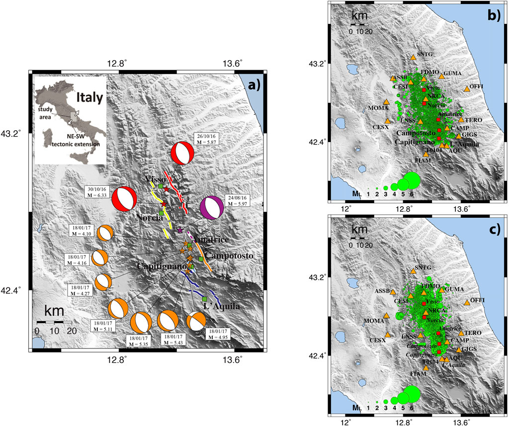
FIGURE 1. Representation of the data set. (A): Mechanisms of selected earthquakes: the mainshocks of Amatrice, Visso and Norcia, and the seven largest events of Capitignano subsequence (from http://eqinfo.eas.slu.edu/eqc/eqc_mt/MECH.IT/). Fault traces are represented by colored lines (fault strands with the same color pertain to the same seismogenic fault system, from Gori et al., 2019). Fault systems are matched with the corresponding focal solutions using the same color; stars correspond to the location of the mainshocks, and green squares represent the main cities of the area. (B) and (C): Locations and magnitudes of the 13,980 earthquakes used in this study (1.1 < M < 6.0) occurred in the time window between 01/01/2012 and 23/08/2016 (B)) and between 24/08/2016 and 05/05/2022 (C)); orange triangles in (B) and (C) indicate the positions of the 21 seismic stations listed in Table S1 of the Supplementary Material.
The AVN seismic sequence contained the largest earthquake ever recorded in the Central Apennines. The sequence was recorded by a relatively dense modern network of seismometers and accelerometers, and the collected data set provides a unique opportunity to study earthquake-related phenomena in the region. Together with the one collected during the 2009 L’Aquila seismic sequence, the AVN data set allows us to study the earthquake sources and the crustal wave propagation with unprecedented accuracy for this region.
The final data set used here for attenuation calculations consists of 13,980 earthquakes recorded by 21 weak-motion 3-component stations belonging to Rete Sismica Nazionale (RSN), run by Istituto Nazionale di Geofisica e Vulcanologia (INGV, Figures 1B,C; see the earthquake catalog provided as a Supplementary Material). A station list, with all the information on the instrumentation installed at each site, is provided as Supplementary Material. The histograms in Figure 2 describe the distributions of: the magnitudes (ML) of the events in our data set, the hypocentral depths, and the hypocentral distances of the recorded seismograms.
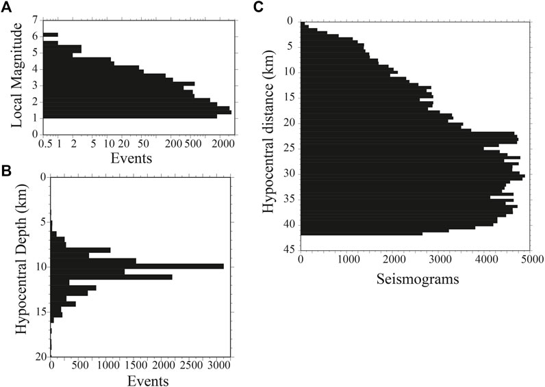
FIGURE 2. Histograms describing our data set: (A) local magnitudes (ML); (B) hypocentral depths, relative to free surface; (C) source-receiver hypocentral distances.
We only used seismograms with one individual event, no glitches, no holes, no spurious noise. Seismograms with multiple (overlapping) events were either cut in the time window containing the specific event only, or removed from the data set. A total of 226,908 high-quality seismograms without glitches, spurious peaks, data gaps, etc., were selected from a data set of over half-a-million time histories generated by 13,980 earthquakes with 1.1 ≤ M ≤ 6.0 occurred between January 1st 2012 and May 5th 2022. Data selection was performed by visually inspecting the individual time histories (done either by Irene Munafò or Luca Malagnini). A signal-to-noise (S/N) ratio analysis was performed on the spectral content of each individual seismogram, as described by Malagnini et al. (2000). Also, during the sequence the magnitudes of the events in the data set are higher (and so is the S/N ratio). Finally, we used Random Vibration Theory in order to maximize the S/N ratio (we use peak values, not spectral amplitudes, see Malagnini and Dreger, 2016 for details).
By using peak amplitude ratios obtained (via a formal regression) at two different, arbitrary hypocentral distances of 40 and 15 km we eliminate most issues related either to site misbehaviors or to variations of source characteristics (i.e., different stress drops) over time. A visual example of unfiltered ground velocity recording, and some of its narrowband-filtered counterparts, is given in Figure 3.
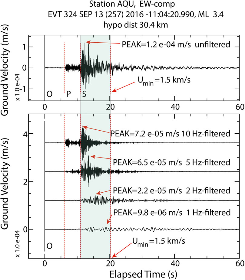
FIGURE 3. Filtering underwent by each seismogram of the data set, before harvesting peak values at a set of central frequencies. Top frame: unfiltered time history. Bottom frame: narrowband-filtered versions of the seismogram at four central frequencies (
Changes in the distribution of the recording sites over time is avoided by choosing to investigate a relatively small crustal volume, which includes only events within 30 km of either Amatrice, Visso, or Norcia, and a fixed set of stations (see list in the Supplementary Material). Among such data set, we selected only waveforms relative to crustal paths with a maximum length of 42 km.
2.2 Methods and related discussion
The technique used here evolved from the work by Raoof et al. (1999) and Malagnini et al. (2000), and its current setting is described by Malagnini et al. (2019) and Malagnini and Parsons (2020). The approach is based on a tool called Random Vibration Theory (RVT) developed by Cartwright and Longuet-Higgins (1956) for the analysis of tides, and subsequently widely used in ground motion analyses (e.g., Boore and Joyner, 1984). We chose to use RVT in order to beat down uncertainties, which is crucial in trying to make precise estimates of 1/Q as a function of time, in a wide frequency band. In fact, RVT allows the use of peak values of narrowband-filtered time histories in place of their Fourier amplitudes (for a detailed explanation, see Malagnini and Dreger, 2016, their Appendix A). Exchanging Fourier amplitudes for peak values brings a huge improvement of the signal-to-noise ratios of the data used in the regressions, which is key in studying the fluctuations of such a feeble parameter as the one that quantifies seismic attenuation. Finally, peak values are obtained from individual-component, geographically-oriented seismograms.
The disadvantage of using RVT is that we lose the information on the peak arrival time, because in theory the peak can occur anywhere in the time history. We worked around this drawback in two ways (a): we prescribed that the analysis be performed in the time window marked by the S-wave arrival, and by an arbitrary minimum group velocity of 1.5 km/s (see Figure 3); (b): we visually inspected all the seismograms of the data set. We gathered progressive groups of 40 consecutive earthquakes from our catalog by moving forward one earthquake at a time: the total number of investigated time windows is:
The issue of stability of the results vs. their time resolution is not important during a seismic sequence, when events are frequent, large, and each of them is recorded by many stations. The issue becomes more important during “regular” times, when earthquakes are infrequent, small, and do not have many recordings. By selecting smaller events, down to ML 1.1, we could gather a sufficient number of earthquakes to allow a relatively constant time resolution (Figure 4A shows the time histories of the total attenuation at the central frequencies of 1.0 and 30.0 Hz, whereas Figure 4B shows a 2-D representation of the attenuation parameter
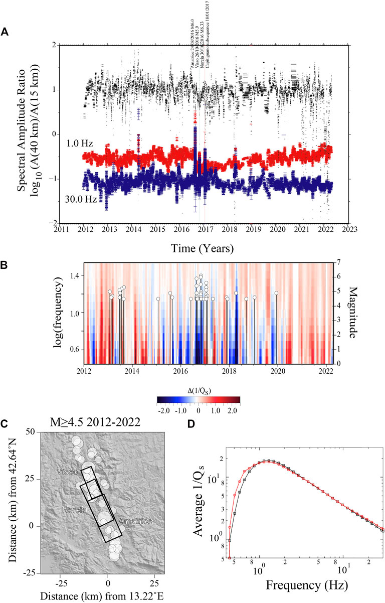
FIGURE 4. (A) Colored symbols: logarithm (base 10) of total attenuation (geometric and anelastic) calculated as a spectral amplitude ratio between the hypocentral distances of 15 and 40 km: before, during, and after the 2016–2017 sequence. Minuscule, horizontal black segments represent the durations of all the m time windows (each one contains 40 events) used to scan the entire period. Horizontal black segments go up and down in order not to overlap; no physical meaning to their elevation: they just follow (amplified) the fluctuations of the 1 Hz attenuation time series. Indicated are the times of occurrence of the main shocks of Amatrice, Visso and Norcia. Note the different behaviors shown by the total attenuation at 1.0 and 30 Hz: whereas the high-frequency time history stays relatively constant throughout the entire period, the 1-Hz one is characterized by a sharp decrease at the onset of the Amatrice main shock, followed by a linear trend of recovery (exponential healing) that appears to be still going on in mid-2022. (B) 2-D representation of the attenuation parameter
In Figure 4C are the epicentral locations of the events with M≥4.5 indicated in Figure 4B, where rectangles indicate the approximate ruptures of the three main shocks of the sequence. Finally, in Figure 4D are the time-averaged attenuation parameters
For each subset of 40 earthquakes we repeat the following steps: 1) filter the
In (1),
The parameter
The n-th row of the matrix (Eq. 1) refers to the n-th observation, the j-th column refers to the j-th seismic source, the i-th column refers to the i-th station, and k=1, … , 44 refers to the k-th regression (one regression per central frequency
Term
The inversion of (1) is performed after adding the following constraints:
where:
Constraints (Eq. 3) effectively decouples the path term (representing total attenuation: geometric and anelastic) from the combination of source and site terms. The reader should keep in mind that our working hypothesis is that the crust is laterally homogeneous in the studied region. Although this hypothesis is never true, it has worked reasonably well in many areas of the world (see studies by Malagnini and others, including those on source scaling, e.g., Mayeda and Malagnini, 2009; Malagnini et al., 2011, Malagnini et al., 2008).
Here we apply constraint (Eq. 4) on horizontal components only, whereas no constraints affect vertical seismograms: it decouples the site and source terms and gives a clear physical meaning to the latter (i.e., the source terms that would be recorded at the reference distance
Constraint (Eq. 5) is a smoothing operator applied to the crustal propagation term, which minimizes the roughness of the solution and has negligible effects on our results. Finally, note that we invert (Eq. 1) using a traditional damped least-squares technique.
For completeness, we note that the number of stations may not be strictly the same for each earthquake, adding some variability from earthquake to earthquake. Yet, they always contribute to the null average site term because the latter is not forced individually on each earthquake, but through the inversion of the matrix (Eq. 1). This is done by adding an extra row of zeros in all columns, except for all columns corresponding to the horizontal site terms, where we insert a large number, comparable to the number of data points. An extra zero is added to the data column.
It is important to note that our choice not to use strong-motion data from the Rete Accelerometrica Nazionale (RAN) contributes to the stability of the results within the time window that comprises the most energetic portion of the 2016–2017 seismic sequence. The RAN accelerograms, however numerous they may be for individual mainshocks, are available only for a handful of larger events. Our choice is based on the fact that we are not interested in source spectra; moreover, the number of available accelerograms is about three orders of magnitude smaller than the total number of seismograms used in this study, and the same proportion holds for the number of earthquakes for which accerelograms were available, compared to the total number of earthquakes.
By inverting matrix (Eq. 1), we obtain one set of source spectra, one set of site terms, and one smooth path term for each central frequency. Because of constraint (Eq. 3), the path term is equivalent to an amplitude ratio between the attenuation at distances
where g(r) is a static attenuation function, piecewise-linear in log-log space,
We can write:
We actually calculate the variations of the attenuation parameter
Figure 4A shows the total attenuation term
We can safely state that above 1 Hz all the peak values of the narrowband-filtered time histories are carried by direct S-waves. To reduce the error bars of the attenuation function, we apply a bootstrap procedure, in which 10% of the events of each time window are removed from the data set. 10 different regressions are run on the data set associated to
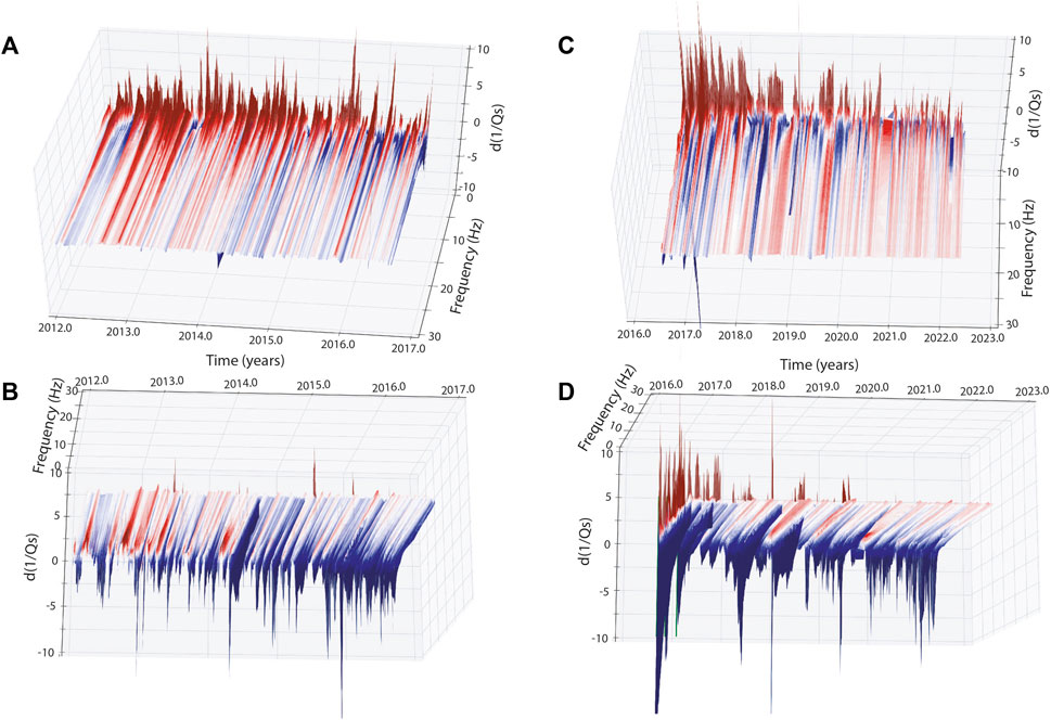
FIGURE 5. Seismic attenuation as a function of time and frequency, calculated at a hypocentral distance of 40 km. 3-D representations of the time-frequency variations of the parameter
By calculating the average attenuation over time, removing the geometric attenuation calculated by Malagnini et al. (2011), their Eq. 3 for the adjacent region that was struck by the 6 April2,009 L’Aquila earthquake, and subtracting it from Eq. 6, we obtain anomalies of
2.3 Limitations of our approach
Scientific results must be thoroughly evaluated to understand hidden limitations of techniques. We point out the existence of issues about the current application developed by Malagnini et al. (2019), and the full extent of their (limited) importance.
2.3.1 Trade-offs
Tradeoffs are the inevitable drawback of any inverse problem. What we have available is Eq. 1, and the constraints that are forced onto the matrix. With such a limited set of tools, we are able to exploit our data set in many different ways, including the assessment of temporal variations of source and site terms (Supplementary Figure S2). Some variability characterizes all terms, but their collective behavior is totally acceptable for our purposes.
Yet, our results must be affected by tradeoffs. As an example, if all sites simultaneously experienced the same amount of damage during some strong shaking, constraint (Eq. 4) would force the changes in site attenuation that are common to all sites, through constraint (Eq. 3), onto all source terms. Because shaking-related rock damage is a shallow consequence of earthquake-induced ground motion, we expect that an increase in site terms occurs at low frequency at the beginning of the sequence. Supplementary Figure S2 documents such a change, which only affects a subset of recording stations and is counterbalanced by the rest of the sites.
The availability of seismometric data in the study area is enough to study the average behavior of the seismic attenuation, and its variability over time. Moreover, the sampled crustal volume (Figure 1) is large enough and well instrumented, so that a large number of stations sample the same crustal volume illuminated by the seismic events. This is especially true for the time window that includes the seismic sequence. In comparison, the time window between 01/01/2012 and 23/08/2016 shows a remarkably constant crustal attenuation pattern (except for the seasonal fluctuations, see Figures 4B, 5), in spite of the fact that in order to obtain enough events to have a decent time resolution in the pre-Amatrice time window we needed to select anything above ML 1.2 (i.e., scattered background seismicity). An even smaller minimum magnitude ML 1.1 was used to sample the 24 days prior to the Amatrice main shock.
Source and site terms are remarkably stable over the period between 01/01/2013 and 23/08/2016 (Supplementary Figure S2), especially when compared to their behaviors during the sequence. It also appears that the more seismically active region of the Central/Northern Apennines between L’Aquila and Norcia, is (in relative terms) seismologically homogeneous, at least in terms of the velocity structure. For example, Malagnini et al., 2011 were successful in using the Central Italy Apennines (CIA) velocity model to reproduce broadband seismograms down to M2.8 - http://www.eas.slu.edu/eqc/eqc_mt/MECH.IT/). The broadband inversion of the moment tensors uses frequencies up to 0.15 Hz, that is, minimum wavelengths of 15–20 km.
We selected a set of stations located within 30 km of any of the mainshocks. Moreover, we always look at the same hypocentral distance of 40 km; recordings collected at distances larger than 40 km could still contribute (mainly through the smoothing constraint (Eq. 5)) to the value of D (r,f), so we decided to limit our data set to hypocentral distances <42 km. We however looked at the same 1/Q plots at shorter and longer hypocentral distances (30 and 80 km, the latter after regressing a different, larger data set containing waveforms recorded at hypocentral distances beyond 100 km), obtaining virtually the same results (Supplementary Figure S3 shows the time variability of 1/Q calculated at a reference distance of 80 km). Finally, regressions demonstrated to be extremely stable to random mislocations that are larger than the location precision (especially to outliers, see Supplementary Figure S4). The various arguments listed in the current subsection concur to establish confidence in our results.
2.3.2 Near-fault and off-fault effects
The effect of seismic attenuation on observed amplitudes of ground motion refers to the integral of all the individual contributions experienced along the entire crustal path, from the immediate vicinity of the fault all the way to the recording site. Because the effect is proportional to the duration that seismic waves are affected by some specific attenuation, we can write that:
As a consequence of (7), the fluctuations of Q in the fault zone could be larger than what we obtain. Note that the near-site contribution
Lastly, we interpret the sharp increase in the seismic attenuation that occurs at low frequency after the onset of the Amatrice mainshock as the effect of rock damage at shallow depths, at or below 1.0 Hz in Figure 2 (lower frame) where surface waves dominate. Due to the nature of surface waves, we expect the effects of shaking-induced rock damage to extend below the free surface, down to less than a few hundred meters.
2.3.3 Causality
We use overlapping subsets of 40 consecutive earthquakes, calculate the attenuation relative to each sub-set, and associate it to a specific time belonging to the time window spanned by the subset (in the current application, it is the time of occurrence of the first earthquake; alternative choices, not shown here, can be the average time, the median time, or even the time of occurrence of the last event). Then the time window is shifted to the next earthquake available along the time axis, and a new subset of 40 earthquakes is obtained by including the 41-st earthquake, and leaving out the first event. The second attenuation data point is calculated and associated to the occurrence time of the second earthquake of the entire data set. There will be times in which the time window spanned by 40 consecutive earthquakes is relatively long, but as soon as the first main shock hits Amatrice, the interevent times get very small, down to a fraction of an hour (Figure 4A).
If the described method is applied without exceptions, when the moving window hits the first mainshock, for 39 more time steps we would include its effects (damage and dilatation reduction) on the resulting attenuation data points, which would all result in a data point associated with an earlier time, with respect to that of the occurrence of the main shock. We would thus have a causality issue for whatever the choice of the occurrence time to associate with a specific data point. In order to avoid the described acausal effects, we broke the data set into two parts: before and after Amatrice. After the first mainshock, although the sampling of the attenuation parameter is fine we apply this procedure to eliminate the acausal effects related to the other two main events (Visso and Norcia), as well as to the Capitignano subsequence.
To aid in interpretation of attenuation observations, we add independent lines of investigation. We calculate coseismic dilatation to gain insight into where post-earthquake extension and compression occur and associated inferred crack opening or closing. We additionally conduct simple calculations of expected changes in relative fluid flow magnitudes and directions based on dilatation. We also examine the catalog for seismic patterns in time and space that are consistent with fluid diffusion signals.
2.3.4 Effects of coseismic dilatation (stress drop)
We calculate the coseismic dilatation caused by earthquakes during the 2016–2017 Amatrice-Visso-Norcia seismic sequence and the Capitignano subsequence by using a boundary element method. We use rupture plane definitions from local moment tensor solutions (see supplement for solutions and dislocations). Elastic dislocations are made from earthquake rupture areas and slip that are scaled according to the empirical regressions of Wells and Coppersmith (1994), and centered at reported hypocenters/centroids. We assume that all the events occurred on the southwest-dipping nodal planes, which are the prevailing known rupture styles. Dilatation calculations are made using the subroutines of Okada (1992). Since we are calculating dilatation strain, no friction coefficient is necessary. Results are shown in Figures 6A,B, with much of the region showing negative dilatation (compression) following the seismic sequences. Additionally, we make calculations of static stress changes on the eventual Visso and Norcia mainshock ruptures utilizing available focal mechanisms of all events beginning with the Amatrice mainshock to immediately before the Visso, and then Norcia events (after Mancini et al., 2019). This is also done using the subroutines of Okada (1992), but rather than a half-space calculation, shear, normal, and Coulomb stress change calculations are resolved on the mainshock failure planes. This is done to assess the relative influence of fluid diffusion vs. direct coseismic triggering within the mainshock sequences.
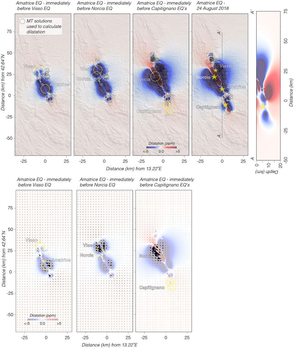
FIGURE 6. Upper Cumulative dilatation. Cumulative dilatation is calculated assuming the SW dipping moment tensor solutions of M≥3 earthquakes were the rupture planes. Dilatation is shown on horizontal planes at 5 km depth, and a cross section is also shown. If drops in
From the visual inspection of Figure 7 we establish that: 1) the attenuation enhancement occurs mostly in the low-frequency end of the investigated band; 2) 1/Q decreases before the Amatrice mainshock, and after the sequence; 3) a positive coseismic jump of the attenuation parameter is evident at the occurrence of the Amatrice main shock; 4) the attenuation parameter returns to a value lower than that observed immediately pre-Amatrice.
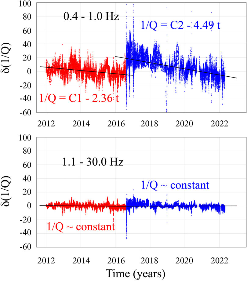
FIGURE 7. Upper: fluctuation of
Calculated changes to fluid flow directions indicate generalized migration of pore fluids away from the most negative dilatancy regions in the crust. Relative magnitudes and directions of radial flow (ur) are calculated using Darcy’s Law assuming porous flow within a confined aquifer as
where k is the permeability of the porous rock, p is pore pressure change, r is radial distance, and
where C represents assumed constants, r0 is the position of the pressure change, and r is the location of an expected flow value at a given distance. We assume changes in dilatancy and/or normal stress are proportional to changes in pore pressure and calculate expected relative flow direction and magnitude from each cell in the model to all the others (Figure 6B).
We searched high-resolution catalogs (Tan et al., 2021) for earthquake sequences in time and space that demonstrate consistency with a diffusion signal. We found that below M3.5, there are too many events likely triggered through multiple processes (e.g., static stress changes, dynamic stress changes, diffusion) to reasonably identify a diffusion process. At thresholds above M3.5 it is possible to systematically search time windows of earthquakes sorted by time and distance from mainshocks to visually identify patterns that could represent diffusion. We then conduct least-squares regressions to see if sequences are well fit to a functional form of
3 Results
3.1 Diffusion signatures on the
Episodes of fluid diffusion are widespread in the Apennines (e.g., Miller et al., 2004; Malagnini et al., 2012). An interesting question is whether they are coupled, in a coincident fashion, with temporal variations of the attenuation parameter. Moreover, it is well known that pulses of pore-fluid pressure may trigger seismic failure by reducing a fault’s shear strength. The mechanism is that the effective fault-normal stress is reduced by the counteracting effect of the fluid pressure (Terzaghi, 1923), thus reducing the fault strength (see, for example, Wang and Manga, 2010), and an interesting scientific question is whether episodes of fluid diffusion (which can possibly cause fault weakening) have detectable signatures on the attenuation parameter. Here we show cumulative evidence to support this from observed temporal changes in seismic attenuation and space-time relations amongst M≥3.5 earthquakes coupled with modeled crustal dilatation, fault-plane stress changes and fluid flow changes.
Following the approach developed by Malagnini et al. (2019), and Malagnini and Parsons (2020), we calculated anomalies of
We note that high frequency waveforms are characterized by small anomalies, indicating that what we detect in our analysis tells us something about the characteristic lengths of the shallow spatial distribution of permeability.
The visual inspection of the time-averaged attenuation (Figure 4D) shows two important aspects of our results: 1) the average anelastic attenuation <1/Q(f)> above 1.0 Hz describes a power law with negative exponent; 2) below roughly 1 Hz, <1/Q(f)> strongly diminishes with diminishing frequency; below 0.4 Hz, the average attenuation plunges to very small, meaningless values. No significant differences are found at high frequencies between the parameter <1/Q(f)> calculated before and after the Amatrice main shock.
It is well-known that surface waves dominate the ground motion at short distance below 1.0 Hz (e.g., Malagnini et al., 2000; Olsen et al., 2006), and so the dimensions of permeability elements (clusters of interconnected cracks) affecting attenuation must be comparable with the 0.4–1.0 Hz wavelengths (1–4 km). At higher frequencies we sample deeper paths because only crustal S-waves enter the calculation, and the characteristic lengths of the permeability heterogeneity distribution are smaller and comparable with the sampling wavelengths. For instance, at around 2 Hz such characteristic length may be between 0.5 and 1.5 km.
The analysis performed over the first 12 h after the Amatrice main event shows three diffusion branches that follow a functional form of
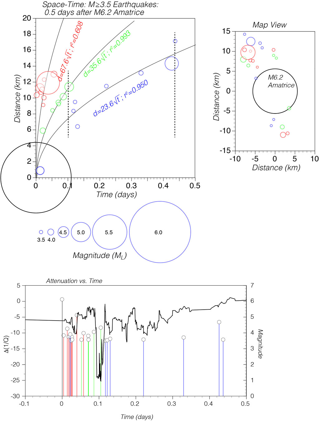
FIGURE 8. Diffusion and attenuation vs. time: Amatrice. Upper: three different simultaneous diffusion processes may be recognized mostly to the North of the Amatrice main shock. Map view to the right. Lower: 2.2 Hz seismic attenuation (black solid line) drops for about 6 h after the mainshock, then goes back to higher values (still negative). The drop in attenuation may be associated to the effect of the coseismic stress drop on the crustal cracks (coseismic crack closure is expected in normal-faulting earthquakes, see Muir-Wood and King, 1993) and thus to crustal permeability. Over a broader time window, the effects are clear and may be interpreted in terms of two competing effects: damage of shallow crustal rocks (Rubinstein and Beroza, 2005), and crack closure due to the coseismic stress drop of a normal-faulting earthquake. The colors of the vertical lines associated with earthquakes correspond with the earthquakes portrayed by colored circles in the upper panel.
As stated by Malagnini et al. (2012) for the M6.1 L’Aquila earthquake of 6 April 2009, and for the sequence of three large aftershocks that occurred on the Campotosto-Monti della Laga and Vettore-Monte Bove faults, it is likely that the tendency of the Apennines to produce diffusive episodes of crustal pore fluids inhibits large main shocks in favor of sequences of multiple, smaller events, because the fault ruptures earlier in its seismic cycle. The time history of the attenuation parameter in one narrow frequency band (2 Hz) is shown in the bottom frame of Figure 8, whereas the high-frequency time history shows fluctuations of moderate amplitude, the 2-Hz waveform shows a marked decrease (to less attenuation) that lasted a bit less than 6 h, followed by a rebound towards normal values. It is interesting that the minimum of
The same analysis is performed on a 10-day period starting at the onset of the Visso main event of 26 October 2016 (Figure 9). The Norcia earthquake (ML 6.5, M 6.33) is also included. The 2 Hz attenuation curve is characterized by a similar behavior as after the Amatrice shock. First, at the onset of each main event, the attenuation parameter plunges steeply, then it bounces back. The time scale is about 20 times wider than that following Amatrice (Figure 8), but the negative-positive swing after each main shock takes about 24 h to complete, which is roughly twice the time it took for the same swing after the Amatrice main event. Figure 10 shows yet another interesting situation, where a separate small seismic sequence hits the Campotosto fault (Falcucci et al., 2018; Cheloni et al., 2019; Gori et al., 2019) with a series of four M5+ events that occurred in less than 5 h. The sequence migrates quickly southward along the fault, with a clear diffusive signature. Potential diffusion pathways are highlighted by microseismicity from the high resolution relocated catalog of Tan et al. (2021), where fault structures are apparent in cross section view (Figure 11).
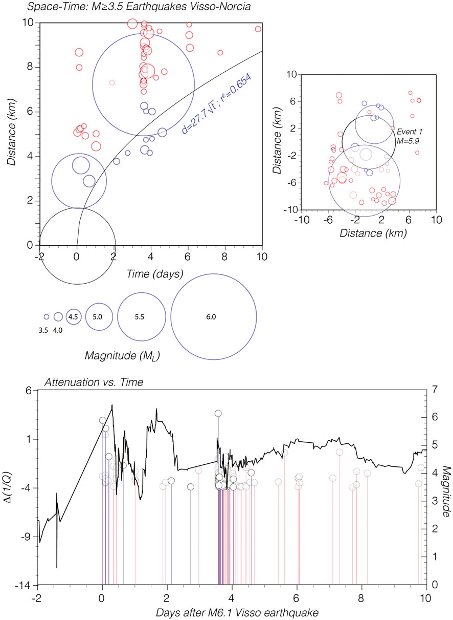
FIGURE 9. Diffusion and attenuation vs. time: Visso-Norcia. Upper: diffusion process associated to the mainshocks of Visso (26 October 2016) and Norcia (30 October 2016), with a map view to the right. Lower: 2.2 Hz fluctuation of the seismic attenuation parameter around the pre-Amatrice average. The colors of the vertical lines associated with earthquakes correspond with the earthquakes portrayed by colored circles in the upper panel.
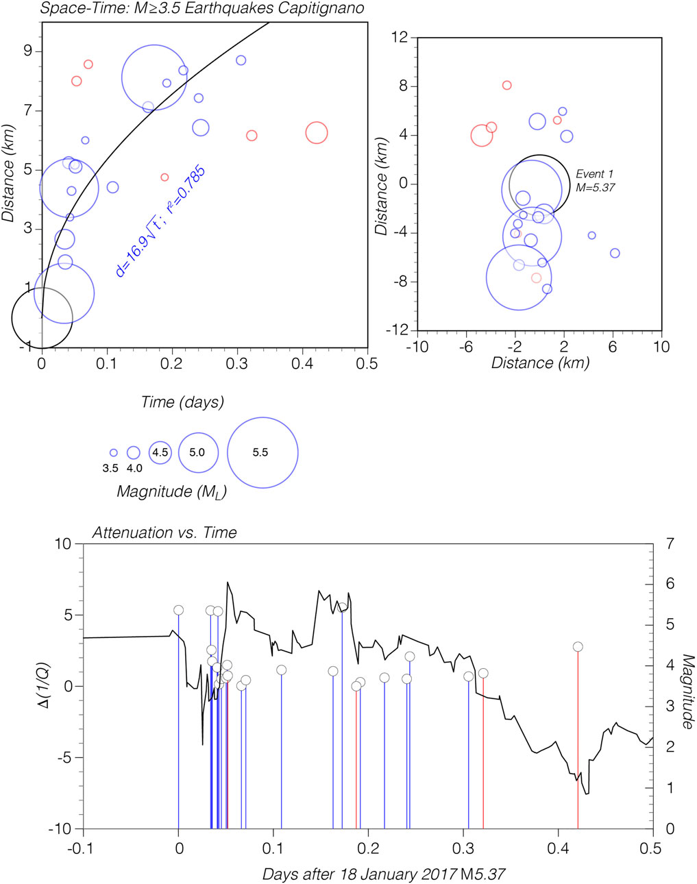
FIGURE 10. Diffusion and attenuation vs. time: Capitignano. Upper: diffusion process associated to the seismic sequence of Capitignano (18 January 2017). Map view to the right. Lower: 2.2 Hz fluctuation of the seismic attenuation parameter around the pre-Amatrice average. The colors of the vertical lines associated with earthquakes correspond with the earthquakes portrayed by colored circles in the upper panel.
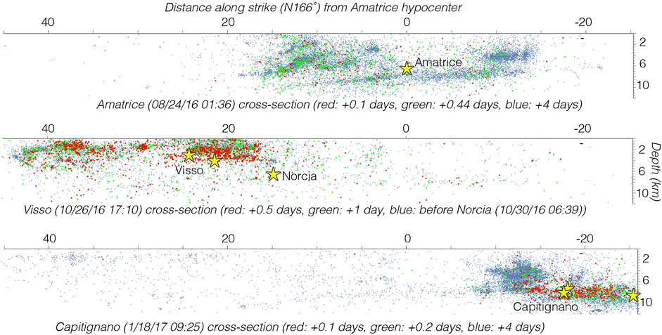
FIGURE 11. Cross-sectional views of relocated catalogs. Relocated earthquake catalogs of the Central Apennines seismic sequence (Tan et al., 2021). The top panel shows an eastward view that highlights a basal detachment at ∼10–15 km depth as well as several structures above it. Red events correspond to the first 0.1 days after the Amatrice mainshock and to the first two diffusion curves in Figure 8, and the green dots include all three diffusion events; these earthquakes highlight potential fluid diffusion pathways along faults. The red events in the center panel correspond in time with the potential diffusion event between the Visso and Norcia shocks (Figure 9). The lower panel shows potential diffusion pathways involving the Capitignano sequence of 4 M≥5 shocks (Figure 10).
In the three cases documented in Figures 8–10, the diffusion coefficient is very large, up to
For a rock compressibility
The estimates of permeability provided above are relative to critically stressed faults that just ruptured, not to the off-fault rock matrix, where we expect that the negative dilatation due to normal-faulting earthquakes would reduce crack density and thus permeability. In other words, the values of permeability found here are relative to the crustal plumbing system in the epicentral region (fault planes outlined by the seismicity in Figure 11), in the sense described by Townend and Zoback (2000), which is contained in a volume in which the bulk permeability has decreased due to the effect of the elastic stress drop from normal faulting earthquakes (Muir-Wood and King, 1993).
Seismic attenuation occurs during propagation through bulk crustal rocks, and is unaffected by the variations of permeability of the regional plumbing network. On the contrary, because episodes of macroscopic diffusion like those documented in Figures 8–10 occur along critically stressed fault planes, their parameters cannot be used to compute rocks’ bulk permeabilities.
3.2 Effects of cumulative dilatation on
In the hypothesis that time-dependent seismic attenuation depends on rock permeability, associations between earthquakes and changes in
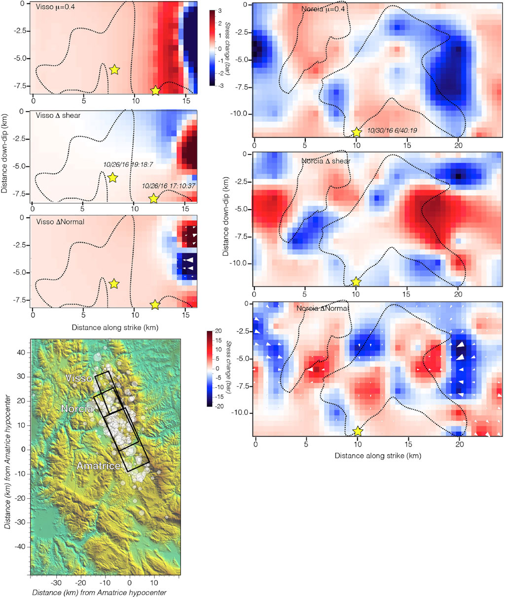
FIGURE 12. Calculated static stress changes from M≥3 earthquakes beginning with the 24 August 2016 Amatrice earthquake resolved on the ruptures of the Visso and Norcia earthquakes (left and right columns, respectively). Hypocenters are shown by yellow stars and approximate slip distributions outlined from solutions by Chiaraluce et al. (2017). Coulomb stress changes are mostly positive on the Visso plane (calculated with an intermediate friction coefficient of 0.4). Shear and normal stress changes are also shown. Expected magnitudes and directions of relative fluid flow resulting from normal stress changes are superposed on the normal stress change map for both the Visso and Norcia ruptures. The Norcia plane shows very complex patterns of stress change and fluid flow.
Similarly, after the Visso mainshock the crust around it is calculated to have a primarily compressive effect with a small gap near the Norcia earthquake (Figure 6A). Calculated fluid flow from just prior to the Norcia mainshock implies flow south towards the Norcia hypocenter as well (Figure 6B). The pattern of static stress change on the Norcia rupture is complex (Figure 12) with about equal areas of Coulomb stress increase and decrease. Areas of peak slip are shown after Chiaraluce et al. (2017), which match reasonably well with the Coulomb stress increases and perhaps slightly better with changes in normal stress. The expected fluid flow on the fault plane from normal stress changes goes towards zones of greatest slip (Figure 12). The dominant postseismic signal is the negative dilatation that is associated with crack closure, and causes fluids to migrate away from these regions (Figure 6B). This model is supported by water level and fluid diffusion observations that were made in the immediate periods following some of the larger earthquakes within the Amatrice-Visso-Norcia and Capitignano sequences (e.g., De Luca et al., 2018; Petitta et al., 2018). Finally, Chiarabba et al. (2009, 2020). Also supported the idea that increased fluid pressure weakened the slip patches of the fault plane of the Norcia main shock.
A striking similarity may be noted between the negative dilatation shown in Figure 6, and the spatial distribution of coda attenuation computed by Gabrielli et al. (2021) (
In an extensional environment, the coseismic stress-drop of a normal-faulting mainshock is expected to produce crack closure in its surrounding volume, with a sudden pore-fluid pressure increase (Muir-Wood and King, 1993). From the upper frame of Figure 7 it is clear that, between 0.4 and 1.0 Hz,
4 Discussion
Multiple physical processes are likely responsible for temporal changes in seismic attenuation, so we must thus consider multiple coseismic effects from earthquakes as we attempt to understand the observed signals that accompany seismicity. If we were to compile a list of all the things that could cause a change in the attenuation parameter
Our results indicate that the attenuation parameter is very sensitive to fluid mobility (intra- and inter-crack) and to fluid saturation, and, together with the theoretical work by O’Connell and Budiansky (1977), strongly support the idea that seismic attenuation is intimately linked to crustal bulk (not fault) permeability. From our results, it follows that crustal permeability is modulated by variations in the compressional stress (e.g., the post-earthquake compression that occurs in normal tectonics, see Muir-Wood and King, 1993), and that fluid viscosity is the reason why a substantial portion of seismic energy goes into heat in the crust. More compression must correspond to less seismic attenuation, and vice-versa. The fact that our analysis is extremely simple, and can be summarized by just Eq. 1, makes artifacts very easy to spot.
Moreover, if permeability and attenuation are linked, then the sudden coseismic increases of
Our calculations show a sizeable and stable overall decrease in the attenuation parameter
It is important to consider that we analyzed seismic attenuation at a hypocentral distance of 40 km, and verified that the variations of 1/Q were virtually identical at a hypocentral distance of 80 km (Supplementary Figure S4), and also at 30 km (not shown). We conclude that the observed variability over time of high-frequency observations of 1/Q must be relatively deep (hypocentral depths are 5–9 km). Because surface waves dominate the seismograms at frequencies f ≤ 1 Hz (see the flattening of the average 1/Q(f) below 1.0 Hz in Figure 4D), our results at low-frequencies must be about a shallower portion of the crust. We can estimate the minimum depth by considering that we use a minimum group velocity of 1.5 km/s, which represents 1.5 km-long wavelengths at 1.0 Hz. A meaningful maximum value for surface-wave group velocities at 1.0 Hz could be around 3 km/s. As a rule-of-thumb, surface waves sample the crust to 1/3 of their length, and so we conclude that, at frequencies below 1 Hz, we obtain information on the attenuation at shallow depths, down to a maximum depth of ∼1 km.
In the immediate aftermath of a mainshock, the competition between shallow rock damage and negative dilatation at depth affects the intermediate frequencies of the sampled bandwidth, where we observe a short-lived increase of the parameter
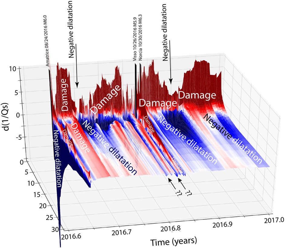
FIGURE 13. Zoom on the 3D visualization of the seismic attenuation parameter
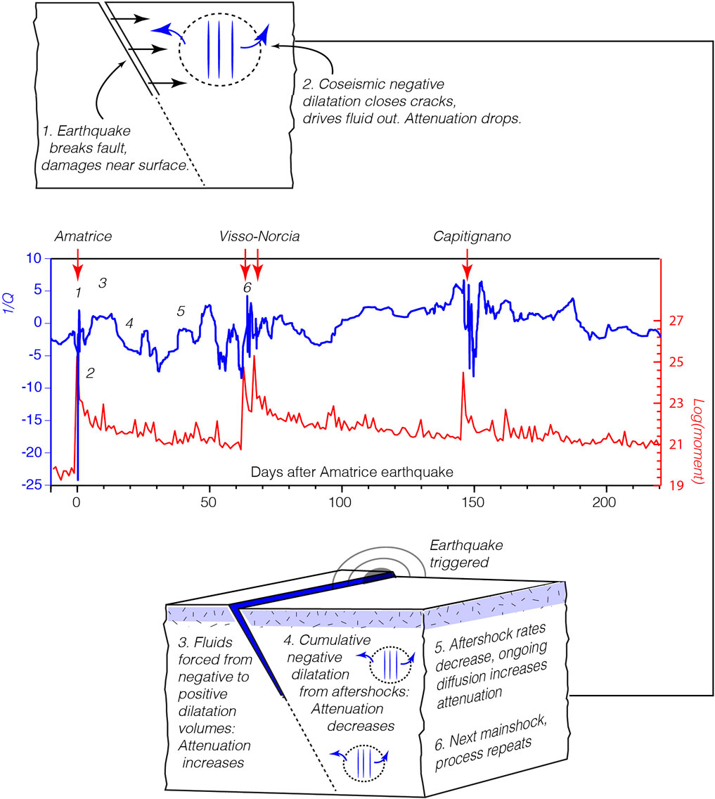
FIGURE 14. Conceptual model of fluid behavior. Scaling the attenuation vs. time curves from after the Amatrice, Norcia, and Capitignano earthquakes, we note a consistent shape. Each mainshock that initiates a sequence is associated with a sharp increase in
4.1 The 2016–2017 seismic sequence of the Central Apennines as a cascade of multiple mainshocks
We argue that a dislocation-induced pressure front generated by a large earthquake and its largest aftershocks could trigger another mainshock on either a nearby structure, or on an adjacent, locked patch of the same fault. The new event could even propagate the pressure front further away, not necessarily in the same direction, starting a cascade of events. In fact, in the multi-mainshock seismic sequences of the Central Apennines, multiple cycles of sudden attenuation drops, and more gentle attenuation recoveries suggest that the various mainshocks occurred after 24 August 2016 may have been triggered by intermittent episodes of fluid migration.
For example, we note that the Visso and Norcia earthquakes both lie on the same diffusion curve (Figure 9), meaning that it is possible that increased fluid pressure played a role in triggering the largest earthquake in the Central Apennines sequence. High-resolution catalogs of relocated earthquakes (e.g., Tan et al., 2021) highlight fault surfaces that likely act as high-permeability fluid pathways (Figure 11). The described mechanism could produce the occurrence of multi-mainshock sequences, in the Central Apennines as well as in any other extensional environment. As hypothesized by Malagnini et al. (2012), the induced fluid migration could also favor the segmentation of a major earthquake in multiple ruptures of smaller magnitudes.
Finally, a similar process could drive the preparatory phase of an isolated mainshock, where an individual fracture grows preferentially at the expense of the rest of the fracture population within the same crustal volume. The resulting reduction in crack porosity, and the generalized closing of fractures and cracks in the volume surrounding the growing fracture would cause a reduction in seismic attenuation, an increase in pore-fluid pressure, and an upward migration of pore fluids. The process culminates with the occurrence of the first main shock. Based on this idea, the upward fluid migration may cause an attenuation reduction at intermediate-to-high frequencies in the deeper volume from which fluids escape (which we observe in Figures 5A,B). We also envision a low-frequency attenuation increase in the volume where the crustal fluids diffuse (Figure 4B). Part of the low-frequency response may be outside the bandwidth available in this study, and so frequencies down to 0.2–0.15 Hz are to be included in the time window that precedes a significant mainshock. Such a bandwidth extension may be possible only in areas with a strong background seismicity. In fact, the minimum magnitude necessary to provide a sufficient sampling in the time window that contains the preparatory phase of an isolated mainshock must be substantially higher than in the M1.1 used here for the Central Apennines.
4.2 Open questions
1. Why is crustal attenuation extremely sensitive to bulk compression/dilatation? Malagnini et al. (2019) used the results by Johnson et al. (2017) and demonstrated that, at 2–4 km in depth on the SAF at Parkfield, the attenuation parameter responds to normal stress cyclic anomalies across the fault of the order of ∼100 Pa. The extreme sensitivity indicates that it is the ground motion noise that dominates the random fluctuations that affect our measurements, and not fluctuations of the physical properties of crustal rocks. Once we reduce the noise to a sufficiently low level, we only see the fluctuations of rock permeability. This demonstrates that other physical properties of crustal rocks are very stable over time. This is especially important for analyzing the effects of long-period stress periodicities, like the ones associated with seasonal loading and unloading from precipitation, multi-year wet-dry cycles, or solid Earth tides.
2. The most important aspect of this research is the potential use of our results for monitoring purposes, in the hope that precursory phenomena of large earthquakes could be detected. In fact, the evolution of the crustal crack distribution yields information about variations in strength of some portions of the crust under mounting tectonic stress, where stress tends to concentrate before a crustal rupture. If observed fluctuations of the attenuation parameter are directly linked to variations in the crack density, the latter must be in direct connection with variations of strength.
Italy already has a high-quality seismic network (the Rete Sismica Nazionale, RSN). If the station density of the RSN was improved by an order of magnitude, we would be able to monitor the variability of the attenuation parameter of small regions of specific interest. At least, it would become possible to monitor localized anomalies in the attenuation parameter. Borehole stations would allow high-quality recordings of small earthquakes, consequently a finer spatial and temporal resolution in our monitoring purposes.
A much denser seismic network made of borehole instruments could produce a huge volume of high-quality recordings, and AI algorithms would have to be developed for the analysis. They could be run in quasi-real time, in parallel with multi-frequency sets of regressions like the one presented here. The goal would be to use such tools to locate attenuation anomalies in space and time, in a quest for precursory phenomena.
5 Conclusion
The characteristics of the attenuation parameter (Figures 4, 5, 13, 14) confirm the conceptual model formulated by Malagnini and Parsons (2020), that the time variations in rock permeability modulate the variability of the attenuation parameter. In fact, Figures 4D, 5, 7 show that the average level of the background attenuation parameter between January 2013 and immediately prior to the onset of the sequence, on 24 August 2016, is higher than the background value after the sequence. Figure 6A shows that the cumulative effect of the seismic sequence (the multiple main shocks) on the study area was a negative dilatation (relative increase in compression); such an effect favored crack closure, and thus the decrease in permeability, and in anelastic attenuation as well (the latter is clearly shown in Figure 7).
The Central Apennines, a region under extensional tectonics, is prone to multi-mainshock seismic sequences behaving like a cascade of several mainshocks: for example the 2016–2017 sequence studied here, the Umbria-Marche sequence (swarm) of 1997–1998 (Amato et al., 1998; Miller et al., 2004), and the episode that occurred during the 2009 L’Aquila-Campotosto-Monti della Laga sequence (Malagnini et al., 2012).
We propose a possible physical mechanism for a cascade of multiple main shocks under extensional tectonics, characterized by two main phases: 1) a pre-seismic phase that lasts up to the first earthquake and 2) an intermediate phase, which may be cycled through several times, one for each subsequent main shock. In the first phase, the dilatancy model (Scholtz, 2019) predicts that at some point the preferential growth of one fracture takes the lead at the expense of the general population of cracks (the latter tend to close during this preliminary phase). Such behavior must have consequences on pore fluid pressure, which changes as stress affects cracks.
Pore-fluid drops imply fault strengthening, which inhibits rupture, whereas pore-fluid pressure rises imply fault weakening, which promotes rupture. In the intermediate phases that start at mainshock onsets, two main physical processes compete in defining the attenuation parameter, rock permeability and pore-fluid pressure. The driving mechanisms are damage and negative dilatation (stress drop). While damage corresponds to a drop in pore-fluid pressure in the shallow crust, negative dilatation and healing correspond to a deeper pore-pressure rise.
Muir-Wood and King (1993) observed that, in an extensional environment, the seismic stress drop of a main event always increases stream discharge, up to an order of magnitude more in volume than a reverse-fault mainshock of the same magnitude. This is because the elastic stress drop tends to close cracks oriented orthogonally to the (horizontal) direction of the minimum principal stress, causing a sudden increase in the pore-fluid pressure. A similar crack closure (pressure rise) may be envisioned in the pre-seismic phase, in which dilatancy predicts the preferential growth of one crack that is favorably oriented to the stress field, at the expense of the general population of cracks that during this preliminary phase tends to close.
Our conceptual model may be described as follows:
1. During the pre-seismic rupture growth in an extensional environment there may be a “slow” localized negative dilatation, crack closure, pore-pressure rise and migration (diffusion) along fault, and a resulting decreased fault strength that leads to the first main rupture. In all that we describe, permeability must be low enough to support local pore pressure increases, probably over a time scale of several months.
2. The first main event produces coseismic damage and negative dilatation: while the first phenomenon causes a short-lived fluid pressure drop, the second causes a persistent fluid pressure rise; 1/QS shows opposite behavior. In turn, the fluid pressure rise and migration (diffusion) is responsible for the strength reduction in nearby faults, and the occurrence of the next earthquake. The cycling over a cascade of main events ends when the system is depleted of its elastic energy below a certain threshold, when it is not able to produce any more ruptures.
Data availability statement
Publicly available datasets were analyzed in this study. This data can be found here: https://www.orfeus-eu.org/data/eida/.
Author contributions
LM: Coding for attenuation analysis, data quality control, computation of the attenuation parameter, interpretation of results, manuscript preparation; TP: Computation of crustal dilatation, interpretation of results, manuscript editing; IM: Data quality control, interpretation of results, manuscript editing; SM: Computation of stress variations on the fault planes, manuscript editing; MS: Computation of stress variations on the fault planes, manuscript editing; ELG: 3-D analysis of the seismicity, manuscript editing.
Funding
Progetti INGV di Ricerca Libera 2019 (LM), Progetto INGV “Pianeta Dinamico” (LM), Centro di Pericolosità Sismica, Triennio 2019–2021 Convenzione B1 Dipartimento della Protezione Civile—INGV (IM).
Conflict of interest
The authors declare that the research was conducted in the absence of any commercial or financial relationships that could be construed as a potential conflict of interest.
Publisher’s note
All claims expressed in this article are solely those of the authors and do not necessarily represent those of their affiliated organizations, or those of the publisher, the editors and the reviewers. Any product that may be evaluated in this article, or claim that may be made by its manufacturer, is not guaranteed or endorsed by the publisher.
Supplementary material
The Supplementary Material for this article can be found online at: https://www.frontiersin.org/articles/10.3389/feart.2022.963689/full#supplementary-material
References
Akinci, E., Del Pezzo, E., and Malagnini, L. (2020). Intrinsic and scattering seismic wave attenuation in the Central Apennines (Italy). Phys. Earth Planet. Interiors 303, 106498. doi:10.1016/j.pepi.2020.106498
Amato, A., Azzara, R., Chiarabba, C., Cimini, G. B., Cocco, M., Di Bona, M., et al. (1998). The 1997 umbria-marche, Italy, earthquake sequence: A first look at the main shocks and aftershocks. Geophys. Res. Lett. 25, 2861–2864. doi:10.1029/98gl51842
Barbosa, N. D., Hunziker, J., Lissa, S., H Saenger, E., and Lupi, M. (2019). Fracture unclogging: A numerical study of seismically induced viscous shear stresses in fluid-saturated fractured rocks. J. Geophys. Res. Solid Earth 124 (11), 11705–11727. doi:10.1029/2019JB017984
Boore, D. M., and Joyner, W. B. (1984). A note on the use of random vibration theory to predict peak amplitudes of transient signals. Bull. Seismol. Soc. Am. 74 (5), 2035–2039. doi:10.1785/bssa0740052035
Brodsky, E. E., Roeloffs, E., Gall, D. I., and Manga, M. (2003). A mechanism for sustained groundwater pressure changes induced by distant earthquakes. J. Geophys. Res. 108, 2390. doi:10.1029/2002jb002321
Cartwright, D. E., and Longuet-Higgins, M. S. (1956). The statistical distribution of the maxima of a random function. Proc. R. Soc. Lond. A 237, 212–232. doi:10.1098/rspa.1956.0173
Cheloni, D., D’Agostino, N., Scognamiglio, L., Tinti, E., Bignami, C., Avallone, A., et al. (2019). Heterogeneous behavior of the Campotosto normal fault (central Italy) imaged by InSAR GPS and strong-motion data: Insights from the 18 january 2017 events. Remote Sens. (Basel). 11, 1482. doi:10.3390/rs11121482
Chen, K. H., Furumura, T., and Rubinstein, J. (2015). Near-surface versus fault zone damage following the 1999 Chi-Chi earthquake: Observation and simulation of repeating earthquakes. J. Geophys. Res. Solid Earth 120 (4), 2426–2445. doi:10.1002/2014JB011719
Chiarabba, C., De Gori, P., Segou, M., and Cattaneo, M. (2020). Seismic velocity precursors to the 2016 Mw 6.5 Norcia (Italy) earthquake. Norcia (Italy) Earthq. Geol. 48 (9), 924–928. doi:10.1130/G47048.1
Chiarabba, C., Piccinini, D., and De Gori, P. (2009). Velocity and attenuation tomography of the Umbria Marche 1997 fault system: Evidence of a fluid-governed seismic sequence. Tectonophysics 476, 73–84. doi:10.1016/j.tecto.2009.04.004
Chiaraluce, L., Di Stefano, R., Tinti, E., Scognamiglio, L., Michele, M., Casarotti, E., et al. (2017). The 2016 central Italy seismic sequence: A first look at the mainshocks, aftershocks, and source models. Seismol. Res. Lett. 88, 757–771. doi:10.1785/0220160221
Convertito, V., De Matteis, R., Improta, L., and Pino, N. A. (2020). Fluid-triggered aftershocks in an anisotropic hydraulic conductivity geological complex: The case of the 2016 Amatrice sequence, Italy. Front. Earth Sci. (Lausanne). 8, 541323. doi:10.3389/feart.2020.541323
De Luca, G., Di Carlo, G., and Tallini, M. (2018). A record of changes in the Gran Sasso groundwater before, during and after the 2016 Amatrice earthquake, central Italy. Sci. Rep. 8, 15982. doi:10.1038/s41598-018-34444-1
Falcucci, E., Gori, S., Bignami, C., Pietrantonio, G., Melini, D., Moro, M., et al. (2018). The Campotosto seismic gap in between the 2009 and 2016-2017 seismic sequences of central Italy and the role of inherited lithospheric faults in regional seismotectonic settings. Tectonics 37, 2425–2445. doi:10.1029/2017TC004844
Gabrielli, S., Akinci, A., Ventura, G., Napolitano, F., Del Pezzo, E., and De Siena, L. (2021). Changes in seismic attenuation due to fracturing and fluid migration during the 2016-2017 Central Italy seismic sequence. JGR Solid Earth. Published Online: Thu, 29 Jul 2021. doi:10.1002/essoar.10507643.1
Galluzzo, D., La Rocca, M., Margerin, L., Del Pezzo, E., and Scarpa, R. (2015). Attenuation and velocity structure from diffuse coda waves: Constraints from underground array data. Phys. Earth Planet. Interiors 240, 34–42. doi:10.1016/j.pepi.2014.12.004
Gori, S., Munafò, I., Falcucci, E., Moro, M., Saroli, M., Malagnini, L., et al. (2019). Active faulting and seismotectonics in central Italy: Lesson learned from the past 20 years of seismicity. in Engineering clues Earthquake geotechnical engineering for protection and development of environment and constructions-silvestri & moraci. Editors F. Silvestri, and N. Moraci (Boca Raton, Florida, United States: CRC Press). ISBN 978-0-367-14328-2.
Hanks, T. C. (1982). Bulletin of the seismological society of America. fmax. 72 (6A), 1867–1879. doi:10.1785/BSSA07206A1867
Hoshiba, M. (1995). Estimation of nonisotropic scattering in Western Japan using coda wave envelopes' Application of a multiple nonisotropic scattering model. J. Geophys. Res. 100 (B1), 645–657. doi:10.1029/94jb02064
Johanson, I. A., and Bürgmann, R. (2010). Coseismic and postseismic slip from the 2003 San Simeon earthquake and their effects on backthrust slip and the 2004 Parkfield earthquake. J. Geophys. Res. 115, B07411. doi:10.1029/2009JB006599
Johnson, C. W., Fu, Y., and Bürgmann, R. (2017). Stress models of the annual hydrospheric, atmospheric, thermal, and tidal loading cycles on California faults: Perturbation of background stress and changes in seismicity. J. Geophys. Res. Solid Earth 122 (10), 605. doi:10.1002/2017JB014778
Kelly, C. M., Rietbrock, A., Faulkner, D. R., and Nadeau, R. M. (2013). Temporal changes in attenuation associated with the 2004 M6.0 Parkfield earthquake. J. Geophys. Res. Solid Earth 118, 630–645. doi:10.1002/jgrb.50088
Kilb, D., Biasi, G., Anderson, J., Brune, J., Peng, Z., and Vernon, F. L. (2012). A comparison of spectral parameter kappa from small and moderate earthquakes using southern California ANZA seismic network data. Bull. Seismol. Soc. Am. 102 (1), 284–300. doi:10.1785/0120100309
Liu, W., and Manga, M. (2009). Changes in permeability caused by dynamic stresses in fractured sandstone. Geophys. Res. Lett. 36, L20307. doi:10.1029/2009GL039852
Malagnini, L., Akinci, A., Mayeda, K., Munafo’, I., Herrmann, R. B., and Mercuri, A. (2011). Characterization of earthquake-induced ground motion from the L’Aquila seismic sequence of 2009, Italy. Geophys. J. Int. 184, 325–337. doi:10.1111/j.1365-246X.2010.04837.x
Malagnini, L., Dreger, D. S., Bürgmann, R., Munafò, I., and Sebastiani, G. (2019). Modulation of seismic attenuation at Parkfield, before and after the 2004 M6 earthquake. J. Geophys. Res. Solid Earth 124, 5836–5853. doi:10.1029/2019JB017372
Malagnini, L., and Dreger, D. S. (2016). Generalized free-surface effect and random vibration theory: A new tool for computing moment magnitudes of small earthquakes using borehole data. Geophys. J. Int. 206, 103–113. doi:10.1093/gji/ggw113
Malagnini, L., Herrmann, R. B., and Di Bona, M. (2000). Ground motion scaling in the Apennines (Italy). Bull. Seismol. Soc. Am. 90, 1062–1081. doi:10.1785/0119990152
Malagnini, L., Lucente, F., De Gori, P., Akinci, A., and Munafo', I. (2012). Control of pore-fluid pressure diffusion on fault failure mode: Insights from the 2009 L'aquila seismic sequence. J. Geophys. Res. 117, 0148–0227. doi:10.1029/.2011JB008911
Malagnini, L., and Parsons, T. (2020). Seismic attenuation monitoring of a critically stressed San Andreas fault. Geophys. Res. Lett. 47, e2020GL089201. doi:10.1029/2020GL089201
Mancini, S., Segou, M., Werner, M. J., and Cattania, C. (2019). Improving physics-based aftershock forecasts during the 2016-2017 central Italy earthquake cascade. J. Geophys. Res. Solid Earth 124, 8626–8643. doi:10.1029/2019JB017874
Manga, M., Beresnev, I., Brodsky, E. E., Elkhoury, J. E., Elsworth, D., Ingebritsen, S. E., et al. (2012). Changes in permeability caused by transient stresses: Field observations, experiments, and mechanisms. Rev. Geophys. 50, RG2004. doi:10.1029/2011RG000382
Manga, M., and Brodsky, E. (2006). Seismic triggering of eruptions in the far field: Volcanoes and geysers. Annu. Rev. Earth Planet. Sci. 34, 263–291. doi:10.1146/annurev.earth.34.031405.125125
Mayeda, K., and Malagnini, L. (2009). Apparent stress and corner frequency variations in the 1999 Taiwan (Chi‐Chi) sequence: Evidence for a step-wise increase at MW 5.5. Geophys. Res. Lett. 36, L10308. doi:10.1029/2009GL037421
Miller, S., Collettini, C., Chiaraluce, L., Cocco, M., Barchi, M., and Kaus, B. J. P. (2004). Aftershocks driven by a high-pressure CO2 source at depth. Nature 427, 724–727. doi:10.1038/nature02251
Mitchell, B. J. (1995). Anelastic structure and evolution of the continental crust and upper mantle from seismic surface wave attenuation. Rev. Geophys. 33 (4), 441–462. doi:10.1029/95RG02074
Muir-Wood, R., and King, G. C. P. (1993). Hydrological signatures of earthquake strain. J. Geophys. Res. 98 (B12), 22035–22068. doi:10.1029/93jb02219
Noir, J., Jacques, E., Békri, S., Adler, P. M., Tapponnier, P., and King, G. C. P. (1997). Fluid flow triggered migration of events in the 1989 Dobi Earthquake sequence of central Afar. Geophys. Res. Lett. 24 (18), 2335–2338. doi:10.1029/97GL02182
Nur, A., and Booker, J. R. (1971). Aftershocks caused by pore fluid flow? Science 175, 885–887. doi:10.1126/science.175.4024.885
O’Connell, R. J., and Budiansky, B. (1977). Viscoelastic properties of fluid-saturated cracked solids. J. Geophys. Res. 82, 5719–5735. doi:10.1029/jb082i036p05719
Okada, Y. (1992). Internal deformation due to shear and tensile faults in a half-space. Bulletin Seismological Society America 82 (2), 1018–1040. doi:10.1785/BSSA0820021018
Olsen, K. B., Akinci, A., Rovelli, A., Marra, F., and Malagnini, L. (2006). 3D ground-motion estimation in Rome, Italy. Bull. Seismol. Soc. Am. 96 (1), 133–146. doi:10.1785/0120030243
Parsons, T., Malagnini, L., and Akinci, A. (2017). Nucleation speed limit on remote fluid-induced earthquakes. Sci. Adv. 3 (8), e1700660. doi:10.1126/sciadv.1700660
Petitta, M., Mastrorillo, L., Preziosi, E., Banzato, F., Barberio, M. D., Billi, A., et al. (2018). Water-table and discharge changes associated with the 2016–2017 seismic sequence in central Italy: Hydrogeological data and a conceptual model for fractured carbonate aquifers. Hydrogeol. J. 26, 1009–1026. doi:10.1007/s10040-017-1717-7
Raoof, M., Herrmann, R. B., and Malagnini, L. (1999). Attenuation and excitation of three-component ground motion in southern California. Bull. Seismol. Soc. Am. 89, 888–902. doi:10.1785/bssa0890040888
Roeloffs, (1998). Persistent water level changes in a well near Parkfield, California, due to local and distant earthquakes. J. Geophys. Res. 103, 869–889. doi:10.1029/97jb02335
Rubinstein, J. L., and Beroza, G. C. (2005). Depth constraints on nonlinear strong ground motion from the 2004 Parkfield earthquake. Geophys. Res. Lett. 32, L14313. doi:10.1029/2005GL023189
Scholz, C. (2019). The Mechanics of earthquakes and faulting. Cambridge: Cambridge University Press. doi:10.1017/9781316681473
Silverii, F., D’Agostino, N., Borsa, A. A., Calcaterra, S., Gambino, P., Giuliani, R., et al. (2018). Transient crustal deformation from karst aquifers hydrologyi n the Apennines (Italy). Earth Planet. Sci. Lett. 506, 23–37. doi:10.1016/j.epsl.2018.10.019
Tan, Y. J., Waldhauser, F., Ellsworth, W. L., Zhang, M., Zhu, W., Michele, M., et al. (2021). Machine learning based high resolution earthquake catalog reveals how complex fault structures were activated during the 2016–2017 central Italy sequence. Seismic Rec. 1, 11–19. doi:10.1785/0320210001
Terzaghi, K. (1923). Die Berechnung der Durchassigkeitsziffer des Tones aus dem Verlauf der hydrodynamischen Spannungsercheinungen. Sitzungsber. Akad. Wiss. Wien Math. Naturwiss. Kl. Abt. 2A 132, 105–124.
Tinti, E., Spudich, P., and Cocco, M. (2005). Earthquake fracture energy inferred from kinematic rupture models on extended faults. J. Geophys. Res. 110, B12303. doi:10.1029/2005JB003644
Tisato, N., Quintal, B., Chapman, S., Podladchikov, Y., and Burg, J. P. (2015). Bubbles attenuate elastic waves at seismic frequencies: First experimental evidence. Geophys. Res. Lett. 42, 3880–3887. doi:10.1002/2015GL063538
Titzschkau, T., Savage, M., and Hurst, T. (2010). Changes in attenuation related to eruptions of Mt. Ruapehu Volcano, New Zealand. J. Volcanol. Geotherm. Res. 190 (1–2), 168–178. doi:10.1016/j.jvolgeores.2009.07.012
Townend, J., and Zoback, M. D. (2000). How faulting keeps the crust strong. GEOLOGY 28 (5), 399–402. doi:10.1130/0091-7613(2000)028<0399:hfktcs>2.3.co;2
Tung, S., and Masterlark, T. (2018). Delayed poroelastic triggering of the 2016 october Visso earthquake by the August Amatrice earthquake, Italy. Geophys. Res. Lett. 45, 2221–2229. doi:10.1002/2017GL076453
Turcotte, D. L., and Schubert, G. (1982). Geodynamics: Application of continuum physics to geological problems. Hoboken, NJ: Wiley, 450.
Wang, C.-Y., and Manga, M. (2010). Hydrologic responses to earthquakes and a general metric. Geofluids 10, 206–216. doi:10.1111/j.1468-8123.2009.00270.x
Keywords: attenuation parameter, central apennines, shaking-induced rock damage, negative dilatation, fluid diffusion, rock permeability, random vibration theory
Citation: Malagnini L, Parsons T, Munafò I, Mancini S, Segou M and Geist EL (2022) Crustal permeability changes inferred from seismic attenuation: Impacts on multi-mainshock sequences. Front. Earth Sci. 10:963689. doi: 10.3389/feart.2022.963689
Received: 07 June 2022; Accepted: 25 July 2022;
Published: 08 September 2022.
Edited by:
Ruizhi Wen, China Earthquake Administration, ChinaReviewed by:
Luca De Siena, Johannes Gutenberg University Mainz, GermanyHamoud Beldjoudi, Centre de Recherche en Astronomie Astrophysique et Géophysique (CRAAG), Algeria
Copyright © 2022 Malagnini, Parsons, Munafò, Mancini, Segou and Geist. This is an open-access article distributed under the terms of the Creative Commons Attribution License (CC BY). The use, distribution or reproduction in other forums is permitted, provided the original author(s) and the copyright owner(s) are credited and that the original publication in this journal is cited, in accordance with accepted academic practice. No use, distribution or reproduction is permitted which does not comply with these terms.
*Correspondence: Luca Malagnini, bHVjYS5tYWxhZ25pbmlAaW5ndi5pdA==