Detection of geological boundaries by 3D gravity inversion for density gradients in different directions

The spatial position and dip feature of the density boundary are significant to the study of fault and tectonic frameworks. Edge detection methods generally attach importance to the horizontal position of the boundary, but it is difficult to determine the dip feature expressly. A density gradient inversion method was proposed based on the corresponding relationship among the gravity forward field, forward kernel matrix, and model attributes. The inversion result of this method is that the density gradient value is different from the conventional gravity inversion. It can directly display the 3D distribution features integrated with 3D inversion results of the density gradient in different directions. The theoretical model means that the inversion results can not only identify the horizontal position of the boundary but also qualitatively determine the dip feature of faults. It has been widely applied to fault identification in the Songliao Basin. According to the joint inversion results, the strike feature and the dip feature can be quantitatively and qualitatively identified, respectively, making up for the shortcomings of sparse distribution and poor lateral resolution of existing seismic data.

Introduction

The gravity method is important in detecting the spatial distribution features of underground density and is also an emphasized geophysical prospecting method for regional geological research and energy mineral exploration. In addition, it plays an important role in investigating the geological and structural features of the bedrock, delineating the scope of the sedimentary basin, studying the fluctuation of the sedimentary rock layer or stratigraphic density interface, as well as the volcanic structure, crustal equilibrium, crustal, and upper mantle structure among others. There are many processing methods for boundary recognition and 3D inversion in gravity data processing and interpretation.

One of the important contents of gravity interpretation is to identify the spatial distribution features of geological body boundaries effectively. Gravity anomalies have a high lateral resolution, and gravity cascade belts with different scales often correspond to the boundaries of underground fault structures and geological bodies such as rock and ore bodies. The derivative operation, mathematical statistics, and multi-scale detection use gravity data to identify a geological body boundary. There are many methods based on the derivative operation, such as the vertical derivative method (VDR) (Hood and Mcclure, 1965; Hood and Teskey, 1989), a total horizontal derivative method based on x and y-direction derivatives (THDR) (Grauch and Cordell, 1987), analytical signal amplitude method based on x-, y-, and z-direction derivatives (ASM) (Nabighian, 1972; Nabighian, 1984; Li, 2006), dip angle method based on the ratio calculation of the aforementioned methods (TA) (Miller and Singh, 1994; Wang and Li, 2004), and θ diagram method (Theta Map) (Wijns et al., 2005), among others. The methods based on mathematical statistics include small domain filtering and standard deviation. Scale separation of multi-scale edge detection methods mainly includes the wavelet multi-scale decomposition (Hornby et al., 1999; Yang et al., 2015) and upward continuation transformation (Holden et al., 2000; Yan et al., 2015).

The 3D constrained gravity inversion can reduce the multi-solution of the gravity field inversion by increasing constraint conditions (Boulanger and Chouteau, 2001). When there is enough prior information, the depth and structural features of inversion results conform to the geological cognition (Camacho et al., 2000; Bosch et al., 2006). Different solutions would be obtained when different weighting factors and calculation strategies are used for constraint conditions. The main constraint methods are as follows: 1) depth constraint: it is used to cancel the natural attenuation of the kernel function with depth, eliminate the situation that the inversion density distribution does not conform to the real anomaly source due to its excessive weight near the surface, and then improve the depth resolution (Li et al., 1996, Li et al., 1998; Commer, 2011; Liu et al., 2013); 2) focus constraint: it can depict the boundary features of abnormal bodies, which is convenient for later processing and interpretation (Last et al., 1983; Portniaguine et al., 1999; Zhdanov, 2009; Wang et al., 2022); 3) physical property boundary constraint: to achieve more reasonable inversion physical property distribution, the upper and lower limit constraints of the geological physical property need to be supplemented in the process of physical property inversion, and the inversion density value is forced to be limited within a certain range (Portniaguine et al., 1999; Gao et al., 2017); 4) structural constraints: it can be used for joint constraints between different geophysical attributes, including cross gradient constraints (Gallardo and Meju, 2003; Fregoso and Gallardo, 2009; Gross, 2019) and summative gradient constraints (Molodtsov et al., 2015; Colombo and Rovetta, 2018; Liu and Zhang, 2022); 5) geostatistical constraints: regional geological characteristics and laws and geologists’ understanding of geological conditions can be added to the model (Shamsipour et al., 2010; Geng et al., 2014; Geng et al., 2019a; Geng et al., 2019b).

Random access memory and computing power are essential for large-scale 3D gravity inversion in massive datasets and this could lead to overall inefficiency. Researchers have studied from different perspectives, mainly including 1) dimension reduction methods: decreasing storage space and computation by reducing dimensions, including random sub-domain inversion (Yao et al., 2007), wavelet compression (Li et al., 2010), and polynomial-based inversion (Liu et al., 2019); 2) symmetry processing method: the geometric lattice method reduces the computational complexity by translation invariance of the gravity field forward kernel matrix (Yao et al., 2002). Jing et al. (2019) further realized a fast algorithm with spatial domain calculation accuracy and frequency domain calculation speed by the fast Fourier transform.

The actual geological body boundary is distributed and the boundary features should be studied in a 3D space. The boundary recognition methods are mainly 2D or pseudo-3D (multi-scale) methods; the processing method is used to reduce the dimension after assuming 3D geological density bodies, and the processing results often simplify the features of geological body boundaries. The 3D gravity field inversion is a 3D method in an ideal case, and its processing results can include all density features of geological bodies. A new boundary recognition method, the 3D density gradient inversion method, was proposed to improve the resolution of density boundary recognition. It directly inverts the horizontal density gradient parameter, that is, density boundary, and it has the advantage of flexible use for constraint information. The principle and technology would be explained below, and the application effect of the method would be verified using the theoretical model and measured data.

Density gradient inversion method

Relationship between the density gradient and gravity gradient

Assuming that the underground space is divided into $M\left(M=m\times n\times p\right)$ prism grids, where $m$ and $n$ are the number of grids in the $x$ (north) direction and $y$ (east) direction, respectively, and $p$ represents the number of grids in the z (vertical) direction, $N\left(N=m\times n\right)$ measuring points are observed on the surface and correspond to the center of top surfaces of prisms one by one (Figure 1).

FIGURE 1

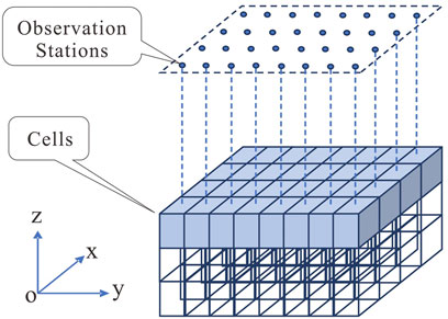
FIGURE 1. One-to-one correspondence between the model element grid and measuring point grid.

According to the forward theory of gravity field, gravity anomaly can be expressed as (Jing et al., 2019).

$\mathbf{d}={\mathbf{F}}^{-1}\left({\sum }_{k=1}^p\mathbf{F}\left({\stackrel{\sim }{\mathbf{G}}}_k\right)\cdot \mathbf{F}\left({\stackrel{\sim }{\mathbf{\rho }}}_k\right)\right),\left(1\le k\le p\right),(1)$

where $\mathbf{d}$ is the gravity anomaly of the model, $\mathbf{F}$ is the forward fast Fourier transform, ${\mathbf{F}}^{-1}$ is inverse fast Fourier Transform, ${\stackrel{\sim }{\mathbf{G}}}_k$ $\left(\left(2m-1\right)\times \left(2n-1\right)\right)$ is the prism forward kernel matrix representing the k-th layer, ${\stackrel{\sim }{\mathbf{\rho }}}_k$ $\left(\left(2m-1\right)\times \left(2n-1\right)\right)$ is the extended matrix after adding zeros to the density matrix of the k-th layer, and $″\cdot ″$ represents the Hadamard product, that is, the multiplication of corresponding elements in two matrixes of the same order.

The first $m\times n$ element in matrix ${\stackrel{\sim }{\mathbf{\rho }}}_k$ is the density matrix element of the k-th layer in the model, and the remaining elements in matrix ${\stackrel{\sim }{\mathbf{\rho }}}_k$ are zero values. The first $m\times n$ element in matrix ${\stackrel{\sim }{\mathbf{G}}}_k$ is the gravity response value of the prism ${\stackrel{\sim }{\rho }}_{m,n,k}$ numbered $\left(m,n\right)$ in the k-th density matrix at the surface measuring point (the default starting number is 1). At this time, the density of the prism ${\stackrel{\sim }{\rho }}_{m,n,k}$ is set to unit density, and the remaining elements in the matrix ${\stackrel{\sim }{\mathbf{G}}}_k$ are stored symmetrically about ${\stackrel{\sim }{\mathrm{G}}}_{m,n,k}$.

Fourier transforms Eq. 1 and multiplies it by the conversion factor $\mathbf{\phi }$ to obtain Eq. 2:

$\mathbf{F}\left({\mathbf{d}}_{\mathbf{\phi }}\right)=\stackrel{\sim }{\mathbf{\phi }}\cdot {\sum }_{k=1}^p\left[\mathbf{F}\left({\stackrel{\sim }{\mathbf{G}}}_k\right)\right]\cdot \mathbf{F}\left({\stackrel{\sim }{\mathbf{\rho }}}_k\right),(2)$

where ${\mathbf{d}}_{\mathbf{\phi }}$ is the gravity conversion field obtained by the conversion factor $\mathbf{\phi }$ of the gravity field, $\mathbf{F}\left({\stackrel{\sim }{\mathbf{d}}}_{\mathbf{\phi }}\right)=\stackrel{\sim }{\mathbf{\phi }}\cdot \mathbf{F}\left(\stackrel{\sim }{\mathbf{d}}\right)$.

When the conversion factor $\mathbf{\phi }$ is a horizontal gradient operator, its expression form is as follows:

${\stackrel{\sim }{\mathbf{\phi }}}_x=\mathit{i}\mathbf{u},(3)$

${\stackrel{\sim }{\mathbf{\phi }}}_y=\mathit{i}\mathbf{v},(4)$

where $\mathbf{u}$ and $\mathbf{v}$ are the wavenumbers in x and y directions, respectively, ${\stackrel{\sim }{\mathbf{\phi }}}_x$ is the x-direction horizontal gradient conversion factor, and ${\stackrel{\sim }{\mathbf{\phi }}}_y$ is the y-direction horizontal gradient conversion factor. Based on the physical meaning, the left term $\mathbf{F}\left({\mathbf{d}}_{\mathbf{\phi }}\right)$ in Eq. 2 represents the horizontal gradient field of gravity in the x-direction or y-direction. When the conversion factor $\stackrel{\sim }{\mathbf{\phi }}$ is combined with density $\stackrel{\sim }{\mathbf{\rho }}$, Eq. 2 is as follows:

$\mathbf{F}\left({\stackrel{\sim }{\mathbf{d}}}_{\mathbf{\phi }}\right)={\sum }_{k=1}^p\mathbf{F}\left({\stackrel{\sim }{\mathbf{G}}}_k\right)\cdot \left[\stackrel{\sim }{\mathbf{\phi }}\cdot \mathbf{F}\left({\stackrel{\sim }{\mathbf{\rho }}}_k\right)\right]={\sum }_{k=1}^p\mathbf{F}\left({\stackrel{\sim }{\mathbf{G}}}_k\right)\cdot \mathbf{F}\left({\stackrel{\sim }{\mathbf{\rho }}}_{\mathbf{\phi }k}\right),(5)$

where ${\stackrel{\sim }{\mathbf{\rho }}}_{\mathbf{\phi }k}$ is the conversion density distribution obtained by the conversion factor $\stackrel{\sim }{\mathbf{\phi }}$ of density distribution ${\stackrel{\sim }{\mathbf{\rho }}}_k$.

Eq. 5 is the relationship between the 3D density gradient and gravity gradient, in which the kernel function is the forward kernel function of the gravity field, which is fixed, and the model parameters can change with the type of observation field.

The model parameter is no longer density, but the horizontal gradient of the density parameter. Generally, the conversion factor may also be used as various conversion filters, such as vertical gradient filters, high-order derivative filters, and combinations of various filters. Different filters can theoretically highlight the different features of the density model and this is not discussed in this study.

For the case where the conversion factor is a horizontal gradient filter, a density model of concealed fracture is set up to visually demonstrate the difference between the density model and the density horizontal gradient model (Figure 2A). The horizontal gradient transformation model of the density model is obtained by summing the horizontal derivatives of the x and y directions of the density model (Figure 2B). Comparing the two models, it can be seen that the density model of concealed fracture consists of two block models and one layered model. After transformation, only one inclined plate remains in the transformed density horizontal gradient model, and the position of the inclined plate is the key feature to identify the fracture model. The horizontal gradient model of the density model can highlight the boundary features of the density model, and this is the significant theoretical foundation of the 3D density gradient inversion.

FIGURE 2

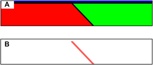
FIGURE 2. Fracture model and the horizontal gradient diagram. (A) Density model of fracture. (B) Horizontal gradient model of fracture density.

Gravity density gradient inversion

In line with the forward-thinking of Eq. 5, the objective function ${\rho }_{\phi }\left(\alpha \right)$ of Tikhonov regularization is constructed (Tikhonov and Arsenin, 1977).

${\rho }_{\phi }\left(\alpha \right)=\left\{{\Vert \mathbf{D}\left({\mathbf{d}}_{\mathbf{\phi }}-\mathbf{G}{\mathbf{\rho }}_{\mathbf{\phi }}\right)\Vert }_2^2+\alpha {\Vert \mathbf{W}\left({\mathbf{\rho }}_{\mathbf{\phi }}-{\mathbf{\rho }}_{\mathbf{\phi }0}\right)\Vert }_2^2\right\},(6)$

where ${\rho }_{\phi }\left(\alpha \right)$ is the expected density model and $\alpha$ is the regularization factor. ${\Vert \mathbf{D}\left({\mathbf{d}}_{\mathbf{\phi }}-\mathbf{G}{\mathbf{\rho }}_{\mathbf{\phi }}\right)\Vert }_2^2$ is the objective function of the fitting difference of gravity transformation data, and the matrix $\mathbf{G}$ is the sensitivity matrix (dimension is $N\times M$), and the elements in the matrix $\mathbf{G}$ corresponds to those in the matrix $\stackrel{\sim }{\mathbf{G}}$ (dimension is $\left(2m-1\right)\times \left(2n-1\right)\times p$) (Yao et al., 2003). ${\Vert \mathbf{W}\left({\mathbf{\rho }}_{\mathbf{\phi }}-{\mathbf{\rho }}_{\mathbf{\phi }0}\right)\Vert }_2^2$ is the objective function of Tikhonov regularization, $\mathbf{D}$ is the diagonal data covariance $N\times N$ matrix (dimension is $N\times N$), and the elements on the diagonal line are the estimated data noise variance. ${\mathbf{\rho }}_{\mathbf{\phi }0}$ is the reference model and $\mathbf{W}$ is the model weighting matrix (dimension is $M\times M$), including the depth weighting matrix and focusing weighting matrix.

Inversion calculation is used to find the minimum solution of the objective function equation (Equation 6). The gradient at the minimum of the objective function must be 0, and the fixed-point iterative equation of the model ${\mathbf{\rho }}_{\mathbf{\phi }}$ in the model space is obtained (Li et al., 2018).

${\mathbf{\rho }}_{\mathbf{\phi }}={\mathbf{\rho }}_{\mathbf{\phi }0}+{\left({\mathbf{G}}^{\mathbf{T}}{\mathbf{D}}^{\mathbf{T}}\mathbf{D}\mathbf{G}+\alpha {\mathbf{W}}^{\mathbf{T}}\mathbf{W}\right)}^{-1}{\mathbf{G}}^{\mathbf{T}}{\mathbf{D}}^{\mathbf{T}}\mathbf{D}\left({\mathbf{d}}_{\mathbf{\phi }}-\mathbf{G}{\mathbf{\rho }}_{\mathbf{\phi }0}\right).(7)$

The density gradient inversion results are obtained using the iterative Eq. 7 inversion calculation. Due to that, the kernel function of this inversion method remains unchanged, only the observation quantity is changed, and the inversion algorithm is consistent with the conventional inversion algorithm. Eq. 7 can also apply an optimization algorithm of 3D gravity inversion for fast inversion calculation of massive data (Jing et al., 2019). It should be noted that the setting of depth weighting function parameters in inversion calculation refers to the values in gravity gradient inversion calculation (Commer, 2011; Qin and Huang, 2016), instead of the values in gravity inversion calculation, and the reference model matrix ${\mathbf{\rho }}_{\mathbf{\phi }0}$ is set to matrix zero.

Calculation process:

(1) Preparing the gravity horizontal gradient data. The gravity data are obtained by the transformation of the 3D equivalent source.

(2) Performing the inversion results of the density gradient in two horizontal gradient directions and obtaining the inversion results of focusing density gradient according to Eq. 7.

(3) Combining the inversion results of the two horizontal gradient models to obtain the final density gradient inversion result.

Model test

The fault zone is a significant geological feature, and the two models, namely, normal fault and reverse fault, are designed to check the effect of the 3D density gradient algorithm on boundary recognition of the fault zone.

Normal fault model test

The normal fault model (Figure 3A) is made up of a north–south strike fault zone (the bottom position of the fault is indicated by dotted lines) and two small anomaly bodies, which have high density in the footwall and low density in the hanging wall. Figures 3B,C show model sections corresponding to lines I and II in Figure 3A, respectively. The underground space is divided into 201 × 121 × 15 prism units of 100 m × 100 m × 100 m. The ground observation data are located in the center of the prism plane, and the data area is the position of the dashed box, totaling 101 × 121 observation data. The gravity forward field (Figure 3D) and the gravity x-direction horizontal gradient forward field (Figure 3E) of the model are taken as the basic fields.

FIGURE 3

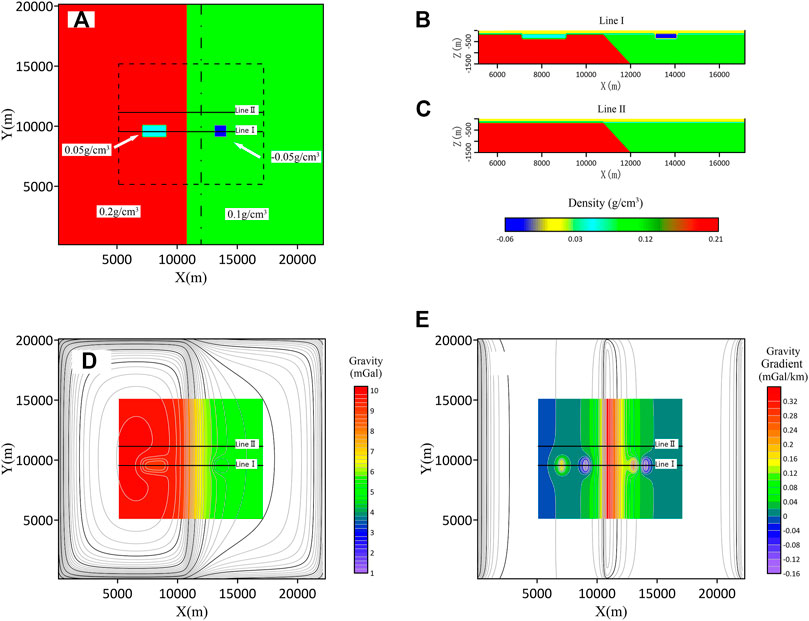
FIGURE 3. Normal fault fracture model and forward modeling field. (A) Model z = −200 m plane distribution map. (B) Model I line position profile; (C) Model II line position profile. (D) Forward gravity modeling results of the model. (E) Forward results of the horizontal gradient in the x-direction of gravity in the model.

The 3D gravity inversion and 3D density gradient inversion of the horizontal gravity gradient in the x-direction are applied in model experiments as well as further focused inversion tests. To facilitate comparison, the inversion results of the 3D density gradient in the model test are represented in absolute values.

The observation data for 3D gravity inversion have the same trend on lines I and II (Figures 4A,D). The anomaly features of gravity data are high in the west and low in the east, in which line I crosses local anomaly bodies, and there are local anomalies in the curve. For the results of unfocused inversion (Figures 4,E), it can be seen that there are longitudinal cascade zones in both sections, and the dip of cascade zones is consistent with the dip of faults (black dotted lines), and the sections of line I show local anomaly bodies to some extent. For the results of focused inversion (Figures 4C,E), it can be seen that the vertical cascade belt in the inversion slice moves down as a whole and becomes relatively gentle, and the recognition of a fault dip becomes blurred.

FIGURE 4

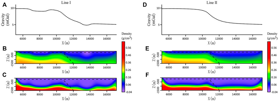
FIGURE 4. Gravity curves and inversion results profiles of line I and line II. (A) Gravity anomaly curve of line I. (B) Slice the inversion result of line I without focusing constraint. (C) Slicing of line I focusing inversion results. (D) Gravity anomaly curve of line II. (E) Slice the inversion result of line II without focusing constraint. (F) Slicing of II line focusing inversion results.

The experimental results show that for the normal fault model, the 3D gravity inversion results are in agreement with the fault dip feature of the theoretical model. However, the focused inversion reduces the coincidence.

The horizontal gradient data of the gravity x-direction for the density gradient inversion have differences in the features of lines I and II (Figures 5A,D). The features of line II data are simple, and its extreme value points correspond well to the fault position, so the horizontal position of a fault can be directly determined. The extreme value points of line I data correspond well to the boundary of the local anomaly body and the position of the fault. However, the amplitude of each extreme value point is close to each other. It is difficult to distinguish the fault zone or the boundary of the local anomaly body directly based on the extreme value points according to the features of the curve. From the results of unfocused inversion (Figures 5B,E), it can be seen that the horizontal position of the fault and the boundary position of the local anomaly are displayed in the section of line I. Although there is a certain indication of a fault dip, the features are not obvious. Section II shows that the horizontal position of the fault is relatively clear, but it does not show the features of the fault dip. From the results of focusing inversion (Figures 5C,F), it can be seen that the profiles of line I and line II clearly depict the fault features, which not only show the horizontal position of the fault but also the fault dip feature, and are close to the fault dip angle of the theoretical model. The boundary of the local anomaly body is clearly depicted by the section of line I.

FIGURE 5

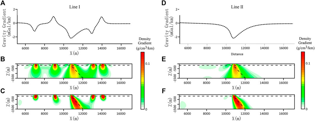
FIGURE 5. Horizontal gravity gradient curve and density gradient inversion result profile in the x-direction of line I and line II. (A) Horizontal gravity gradient anomaly curve of line I. (B) Slice the inversion result of line I without focusing constraint. (C) Line I focusing inversion result slice. (D) Horizontal gravity gradient anomaly curve of line II. (E) Slice the inversion result of line II without focusing constraint. (F) Slicing of line II focusing inversion results.

The model test results show that for the normal fault model, it is difficult to determine the dip feature of faults clearly from 3D density gradient inversion based on the x-direction, and the focus inversion based on the x-direction can enhance the dip features of faults and accurately depict the spatial distribution features of faults, which means that the focus inversion based on the x-direction can directly determine the dip of faults.

Reverse fault model test

The reverse fault model (Figure 6) is also composed of a north–south strike fault zone and two small anomaly bodies, which have a low density in the footwall and high density in the hanging wall. Other parameters are consistent with normal fault model tests. The 3D gravity inversion and horizontal density gradient inversion in the x-direction are designed, as well as the further focused inversion tests.

FIGURE 6

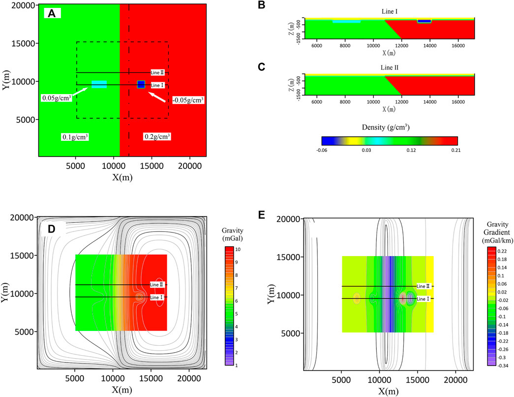
FIGURE 6. Schematic diagram of the reverse fault fracture model. (A) Model z = -200 m plane distribution map. (B) Model line I position profile, (C) Model line II position profile. (D) Forward gravity modeling results of the model. (E) Forward results of the horizontal gradient in the x-direction of gravity in the model.

The gravity inversion data have a similar trend on lines I and II (Figures 7A,D), and the anomaly features of gravity data are low in the west and high in the east, where line I crosses local anomaly bodies. In addition, there are local anomalies in the curve. From the results of unfocused inversion (Figures 7B,E), it can be seen that there are longitudinal cascade zones in both section slices, but the dip of cascade zones is opposite to that of faults (black dotted lines). The section of line I shows the local anomaly body on the east side of the fault to some extent. As for the results of focused inversions (Figures 7C,E), it can be seen that the longitudinal cascade zones in the inversion slices move down as a whole and become relatively gentle, the recognition of fault dip becomes blurred, and the dip feature also indicates reverse direction.

FIGURE 7

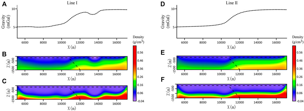
FIGURE 7. Gravity curves and inversion results profiles of lines I and II. (A) Gravity anomaly curve of line I. (B) Slice the inversion result of line I without focusing constraint. (C) Slicing of line I focusing inversion results. (D) Gravity anomaly curve of line II. (E) Slice the inversion result of line II without focusing constraint. (F) Slicing of II line focusing inversion results.

The experimental results show that for the reverse fault model, the 3D gravity inversion and focusing inversion cannot correctly identify the fault dip feature.

The x-direction horizontal gradient data for the density gradient inversion (Figures 8A,D) are consistent with those of the normal fault model, and the main difference is positive and negative symmetries (Figures 5A,D). For the results of unfocused inversion (Figures 8B,E), the section slices of lines I and II indicate the fracture dip to some extent, but the features are not obvious. The boundary of the local anomaly body in the eastern part of the fault can be displayed by the section of line I, but the boundary of the local anomaly body in the western part is weaker. For the results of focusing on inversion (Figures 8D,F), the sections of lines I and II show fracture features, and their dip angles are very close to those of the theoretical model. The section of line I depicts the boundary of the local anomaly body clearly, and it shows the boundary position of the local anomaly body in the east and west of the fault.

FIGURE 8

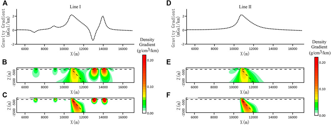
FIGURE 8. Horizontal gradient curve of gravity in the x-direction and inversion result in the profile of the density gradient on line I. (A) Horizontal gravity gradient anomaly curve of line I. (B) Slice the inversion result of line I without focusing constraint. (C) Slicing of line I focusing inversion results. (D) Horizontal gravity gradient anomaly curve of line II. (E) Slice the inversion result of line II without focusing constraint. (F) Slicing of line II focusing inversion results.

To compare with the conventional gravity inversion results, the horizontal gradient inversion calculation in the x-direction is established, and the horizontal derivative in the x-direction is obtained from the inversion density results (Figure 9). When there is no focusing constraint, it can be seen that the section slices of lines I and II (Figures 9B,G) have no indication features for the dip of the fault, and the section slices of line I have a display for the position of the local anomaly body on the east side of the fault, and weak display for that on the west. When the focus constraint is added (Figures 9C,H), the inversion results show that the cascade zone features of the section slices of lines I and II at the fault are ambiguous. The anomaly becomes wide and flat, and it is difficult to identify the transverse position of the fault. However, the position of the local anomaly on the east side of the fault is enhanced, and the local anomaly on the west side of the fault is also enhanced to a certain extent.

FIGURE 9

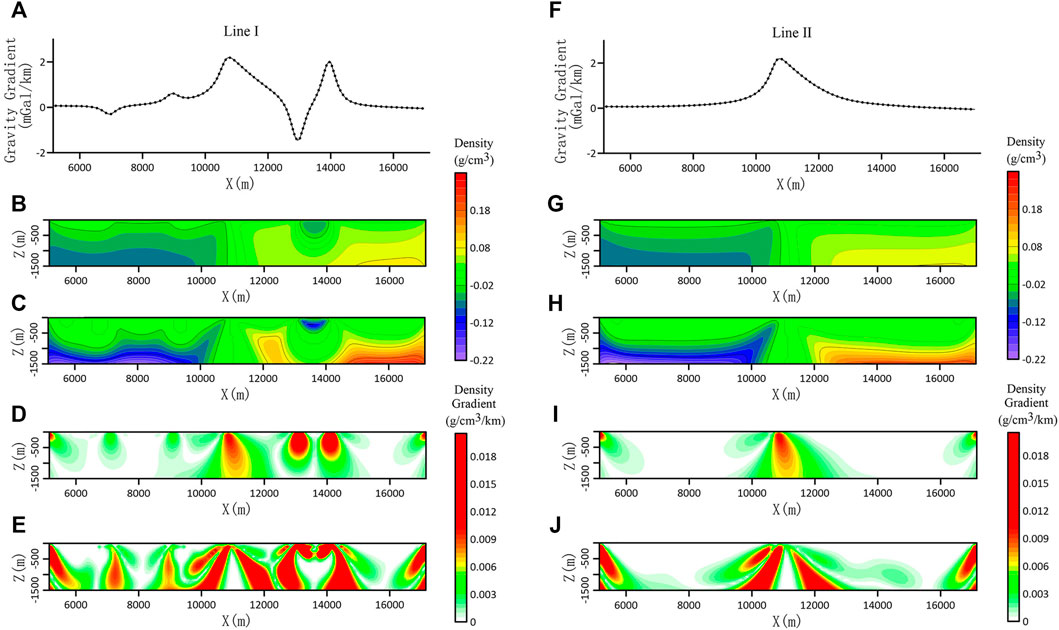
FIGURE 9. Horizontal gravity gradient curve and gradient inversion result profile in the x-direction of lines I and II. (A) Horizontal gradient anomaly curve of gravity in the x-direction on line I. (B) Slice the inversion result of line I without focusing constraint. (C) Slice of line I focusing inversion results. (D) (E) Horizontal derivative in the x-direction of Figures b and c. (F) Horizontal gradient anomaly curve of gravity in the x-direction on line II. (G) Slice the inversion result of line II without focusing constraint. (H) Slice of II line focusing inversion results. (I) (J) Horizontal derivative in the x-direction of images (G) and (H).

The horizontal derivative in the x-direction is obtained from the aforementioned inversion results. Compared with the results of gravity horizontal gradient density gradient inversion (without focusing constraint) (Figures 8B,E), the horizontal gradient results of unfocused inversion (Figures 9D,I) have a slight advantage in depicting faults and abnormal bodies. Compared with the results of gravity horizontal gradient density gradient inversion (focusing constraint) (Figures 8C,F), the horizontal gradient results from focusing constraint inversion (Figures 9E,J) are not only difficult to identify the features of faults and anomaly bodies but also show messy false anomalies. As a result, the experiments indicate that it is difficult to identify the dip features of faults by the gravity horizontal gradient inversion.

The experimental results show that for the reverse fault model, the horizontal position of the fault can be identified by 3D inversion based on the x-direction gravity gradient data, but it is difficult to accurately identify a fault dip feature. The focus inversion of the 3D density gradient based on the x-direction gravity gradient data can enhance the dip features of faults and depict the spatial distribution features of faults.

Application of measured data

The study area is located in the north-central part of the Songliao Basin in China, which is an important oil production base. The research goal was to study the fault structure in this area. This is significant to the study of sedimentation, deformation, hydrocarbon generation, and reservoir formation of basin caprocks on accurately identifying the spatial distribution features of fault structures. The gravity survey work in this study area is relatively up-to-date, and the whole area is covered by medium-scale gravity data. Moreover, the surface is mainly covered by Quaternary deposits, and the terrain is flat; therefore, the gravity anomaly caused by topographic relief can be ignored as shown in Figures 10A,B.

FIGURE 10

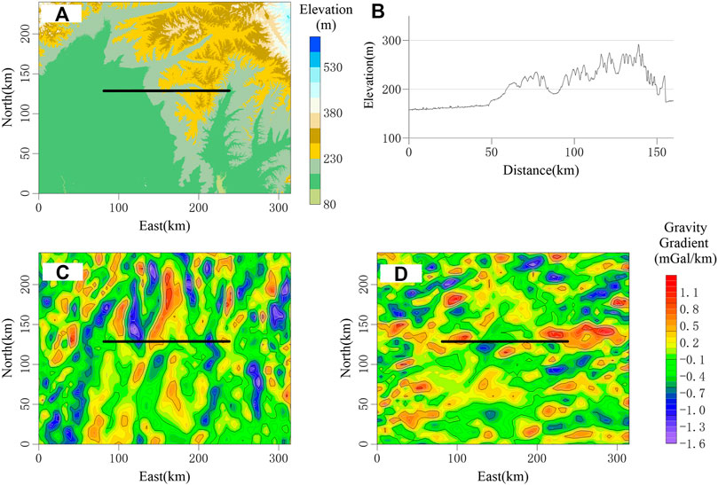
FIGURE 10. Anomaly map of horizontal gravity gradient in the study area. (A) Topographic map of the study area (https://lpdaac.usgs.gov/product_search/?collections=Terra+ASTER&status=Operational&view=list). (B) Topographic data curve at seismic line. (C) Horizontal gravity gradient in the east–west direction. (D) Horizontal gravity gradient in the north–south direction.

Figures 10C,D show the gravity horizontal gradient anomaly in the study area, calculated by the method of 3D equivalent source according to the gravity anomaly data. The structure of the study area is mainly in the north–south direction, and there is evidence that there should be fault zones from the seismic section data, which is a survey line passing through gradient zones at a large angle as shown by the black line in the figure. Figure 11 shows the inversion results of two gradient directions calculated by the method, and the inversion results of the density gradient in the study area are obtained by adding and combining. The results show that the fault development degree in this area is relatively high. The shallow results (Figure 11A) show that the NW-trending fault structure is dominant, middle-shallow results (Figure 11B) show that the NS-trending fault structure is based on the NW-trending fault structure, and middle-deep results (Figure 11C) and deep results (Figure 11D) show that the NNE and NNW-trending faults are dominant, and some EW-trending faults occur.

FIGURE 11

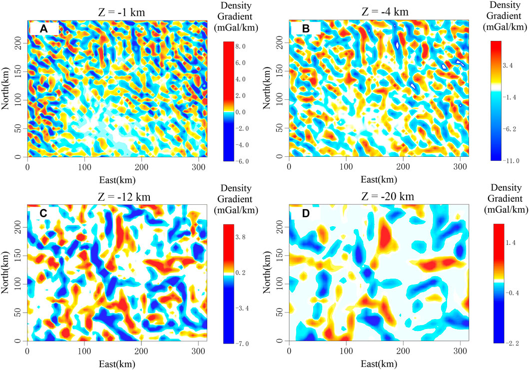
FIGURE 11. Horizontal slices of 3D focusing density gradient inversion results for different vertical depths.

Comparing the interpretation results of the seismic profiles (Figure 12C), gravity anomaly curves (Figure 12A), and gravity horizontal gradient curves (Figure 12B), it can be seen that although the three faults (F1, F2, and F3) have different corresponding relations with the cascade zones or extreme value points in each curve, it is difficult to directly ascertain the dip feature of faults according to these features.

FIGURE 12

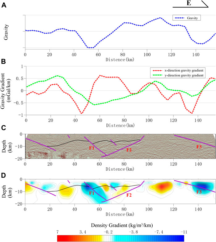
FIGURE 12. Comprehensive interpretation section. (A) Profile gravity anomaly curve. (B) Profile gravity horizontal gradient anomaly curve. (C) Seismic profiles and fault interpretation maps. (D) Inversion result slice and interpretation comparison chart.

Comparing the interpretation results of the inversion section (Figure 12D) and the seismic section (Figure 12C), it can be seen that there is a good corresponding relationship between them: the dip angle of the F3 fault in the seismic section is relatively small, and its spatial position corresponds to the positive and negative anomaly areas in the deep part of the inversion result slice, so it is impossible to judge the dip feature of the fault in the inversion slice. The F2 fault corresponds to the positive anomaly area in the inversion result slice to some extent. Although there is some disposition in the spatial position, the dip features indicated by the F2 fault are similar, and they all dip westward. The position and dip feature of the F1 fault correspond well to the negative anomaly area in the inversion result slice, that is, the F1 fault can be inferred directly from the inversion slice.

The experimental results show that the inversion results of the gravity 3D density gradient can not only identify the transverse distribution features of faults but also identify the vertical features of faults, that is, the dip features of faults. The positions with clear anomaly features in the inversion results have a high degree of coincidence with the results of seismic profile interpretation, showing that this method can identify faults with high reliability. The gravity inversion results based on this method can make up for the shortage of sparse distribution and poor lateral resolution of existing seismic data.

Conclusion

A gravity anomaly inversion method for direct inversion of the density gradient is proposed. The method has the following features:

(1) The parameter of the traditional gravity inversion model is the density attribute, and the parameter of the inversion model is the density gradient attribute. The density gradient model has a more direct correspondence with the density boundary compared with the density model.

(2) The inversion iteration equation and calculation process of this method are almost identical to the conventional gravity inversion method, and all kinds of constraint weighting functions are retained. The main difference is that gravity data are converted into gravity horizontal gradient data, so the cost of programming calculation of this method is minimal, and it is convenient to popularize and apply.

(3) The method adopts a fast algorithm, which can carry out fast inversion calculation of massive gravity data, and the inversion results are relatively stable; hence, this method is expected to become one of the basic methods of gravity processing and interpretation.

(4) The method in this study can only identify the faults with a certain scale, and the inversion results can only show the tendency of the faults. It cannot accurately or quantitatively identify the inclination of the faults.

This method has been successfully applied to fault identification in the northern-central part of the Songliao Basin. The inversion results not only show the different variation features of a fault strike at different depths but also can be directly applied to the identification of fault dip features.

Notably, this study only considers the inversion of the density gradient in two horizontal directions and can discuss the research of the vertical gradient, high-order gradient, and different gradient combinations.

Data availability statement

Requests to access these datasets should be directed to LJ. bGViZXNndWVAMTI2LmNvbQ==

Author contributions

LJ: overall responsible for the method research and numerical simulation of the manuscript. YY: project management. CY: method instruction. LQ: document editing and language polishing. DC: seismic data source. MX: data arrangement.

Funding

This study is financially supported by the National Key R&D Program of China [grant numbers: 2018YFE0208300]. China Geological Survey Project [DD20221639-03; DD20221638; DD20190030]. Engineering innovation and promotion of fine detection technology in deep Geophysical and Chemical exploration.

Acknowledgments

In particular, the authors would like to thank the reviewers and the editor-in-chief for their valuable amendments and suggestions.

Conflict of interest

The authors declare that the research was conducted in the absence of any commercial or financial relationships that could be construed as a potential conflict of interest.

Publisher’s note

All claims expressed in this article are solely those of the authors and do not necessarily represent those of their affiliated organizations, or those of the publisher, the editors, and the reviewers. Any product that may be evaluated in this article, or claim that may be made by its manufacturer, is not guaranteed or endorsed by the publisher.

References

Bosch, M., Meza, R., Jiménez, R., and Hönig, A. (2006). Joint gravity and magnetic inversion in 3D using Monte Carlo methods. Geophys. 71 (4), G153–G156. doi:10.1190/1.2209952

CrossRef Full Text | Google Scholar

Boulanger, O., and Chouteau, M. (2010). Constraints in 3D gravity inversion. Geophys. Prospect. 49 (2), 265–280. doi:10.1046/j.1365-2478.2001.00254.x

CrossRef Full Text | Google Scholar

Camacho, A. G., Montesinos, F. G., and Vieira, R. (2000). Gravity inversion by means of growing bodies[J]. Geophys. 318 (65), 655–664. doi:10.1190/1.1444729

CrossRef Full Text | Google Scholar

Colombo, D., and Rovetta, D. (2018). Coupling strategies in multiparameter geophysical joint inversion. Geophys. J. Int. 215, 1171–1184. doi:10.1093/gji/ggy341

CrossRef Full Text | Google Scholar

Commer, M. (2011). Three-dimensional gravity modelling and focusing inversion using rectangular meshes[J]. Geophys. Prospect. 59 (5), 966–979. doi:10.1111/j.1365-2478.2011.00969.x

CrossRef Full Text | Google Scholar

Fregoso, E., and Gallardo, L. A. (2009). Cross-gradients joint 3d inversion with applications to gravity and magnetic data[J]. Geophysics 74 (4), L31–L42. doi:10.1190/1.3119263

CrossRef Full Text | Google Scholar

Gallardo, L. A., and Meju, M. A. (2003). Characterization of heterogeneous near-surface materials by joint 2d inversion of dc resistivity and seismic data. Geophys. Res. Lett. 30, 1658. doi:10.1029/2003gl017370

CrossRef Full Text | Google Scholar

Gao, X.-H., and Huang, D. N. (2017). Research on 3D focusing inversion of gravity gradient tensor data based on a conjugate gradient algorithm. Chinese J. Geophys. 60 (4), 1571–1583. doi:10.6038/cjg20170429

CrossRef Full Text | Google Scholar

Geng, M., Huang, D., Yang, Q., and Liu, Y. (2014). 3D inversion of airborne gravity-gradiometry data using cokriging. Geophysics 79, G37–G47. doi:10.1190/geo2013-0393.1

CrossRef Full Text | Google Scholar

Geng, M., Welford, J. K., Farquharson, C. G., and Hu, X. (2019a). Gravity modeling for crustal-scale models of rifted continental margins using a constrained 3D inversion method. Geophysics 84, G25–G39. doi:10.1190/geo2018-0134.1

CrossRef Full Text | Google Scholar

Geng, M., Welford, J. K., Farquharson, C. G., and Peace, A. L. (2019b). 3D inversion of airborne gravity gradiometry data for the budgell harbour stock, newfoundland: A case history using a probabilistic approach. Geophysics 84, B269–B284. doi:10.1190/geo2018-0407.1

CrossRef Full Text | Google Scholar

Grauch, V. J. S., and Cordell, L. (1987). Limitations of determining density or magnetic boundaries from the horizontal gradient of gravity or pseudogravity data. Geophysics 52 (1), 118. doi:10.1190/1.1442236

CrossRef Full Text | Google Scholar

Gross, l. (2019). Weighted cross-gradient function for joint inversion with the application to regional 3-d gravity and magnetic anomalies. Geophys. J. Int. 217, 2035–2046. doi:10.1093/gji/ggz134

CrossRef Full Text | Google Scholar

Holden, D. J., Archibald, N. J., Boschetti, F., and Jessell, M. W. (2000). Inferring geological structures using wavelet-based multiscale edge analysis and forward models. Explor. Geophys. 31 (4), 617–621. doi:10.1071/eg00617

CrossRef Full Text | Google Scholar

Hood, P. J., and Teskey, D. J. (1989). Aeromagnetic gradiometer program of the geological survey of Canada. Geophysics 54 (8), 1012. doi:10.1190/1.1442726

CrossRef Full Text | Google Scholar

Hood, P., and Mcclure, D. J. (1965). Gradient measurements in ground magnetic prospecting [J]. Geophysics 30 (3), 403. doi:10.1190/1.1439592

CrossRef Full Text | Google Scholar

Hornby, P., Boschetti, F., and Horowitz, F. (1999). Analysis of potential field data in the wavelet domain. Geophys. J. Int. 137, 175–196. doi:10.1046/j.1365-246x.1999.00788.x

CrossRef Full Text | Google Scholar

Jing, L., Yao, C.-L., Yang, Y.-B., Xu, M. L., Zhang, G. Z., and Ji, R. Y. (2019). Optimization algorithm for rapid 3d gravity inversion[J]. Appl. Geophys. 16 (4), 507–518. doi:10.1007/s11770-019-0781-2

CrossRef Full Text | Google Scholar

Last, B. J., and Kubik, K. (1983). Compact gravity inversion[J]. Geophys. 48 (48), 713. doi:10.1190/1.1441501

CrossRef Full Text | Google Scholar

Li, X. (2006). Understanding 3d analytic signal amplitude [J]. Geophysics 71 (2), l13–l16. doi:10.1190/1.2184367

CrossRef Full Text | Google Scholar

Li, Y., and Oldenburg, D. W. (1996). 3-D inversion of magnetic data. Geophys. 61 (2), 394–408. doi:10.1190/1.1443968

CrossRef Full Text | Google Scholar

Li, Y., and Oldenburg, D. W. (1998). 3-D inversion of gravity data. Geophys. , 63 (1), 109–119. doi:10.1190/1.1444302

CrossRef Full Text | Google Scholar

Li, Y., Oldenburg, D. W., Wei, C., Wang, H., Sui, N., and Kirouac, G. J. (2010). Orexins in the paraventricular nucleus of the thalamus mediate anxiety-like responses in rats. Psychopharmacology 152 (2), 251–265. doi:10.1007/s00213-010-1948-y

PubMed Abstract | CrossRef Full Text | Google Scholar

Li, Z. L., Yao, C. L., and Zheng, Y.-M. (2018). Joint inversion of surface and borehole magnetic amplitude data. Chin. J. Geophys. (in Chinese) 61 (12), 4942–4953. doi:10.6038/cjg2018l0618

CrossRef Full Text | Google Scholar

Liu, J., Zhang, J., Jiang, L., Lin, Q., and Wan, L. (2019). Polynomial-based density inversion of gravity anomalies for concealed iron-deposit exploration in North China. Geophysics 84 (5), b325–b334. doi:10.1190/geo2018-0740.1

CrossRef Full Text | Google Scholar

Liu, J., and Zhang, J.-Z. (2022). Structure-guided gravity inversion for layered density modeling with an application in the Chezhen Depression, Bohai Bay Basin. Geophysics 87 (1), B45–B56. doi:10.1190/geo2021-0213.1

CrossRef Full Text | Google Scholar

Liu, Y. P., Wang, Z. W., Du, X. J., Liu, Q. H., and Xu, J. S. (2013). 3D constrained inversion of gravity data based on Extrapolation Tikhonov regularization algorithm. Chinese J. Geophys. (in Chinese) 56 (5), 1650–1659. doi:10.6038/cjp20130522

CrossRef Full Text | Google Scholar

Miller, H. G., and Singh, V. (1994). Potential field tilt—A new concept for location of potential field sources. Journal of applied geophysics 32 (2-3), 213. doi:10.1016/0926-9851(94)90022-1

CrossRef Full Text | Google Scholar

Molodtsov, D., Colombo, D., Roslov, Y. V., Troyan, V. N., and Kashtan, B. M. (2015). Comparison of structural constraints for seismic-MT joint inversion in a subsalt imaging problem. saint petersburg state university bulletin 2 (3), 230–236.

Google Scholar

Nabighian, M. N. (1972). The analytic signal of two-dimensional magnetic bodies with polygonal cross-section: Its properties and use for automated anomaly interpretation. Geophysics 37 (3), 507. doi:10.1190/1.1440276

CrossRef Full Text | Google Scholar

Nabighian, M. N. (1984). Toward a three-dimensional automatic interpretation of potential field data via generalized Hilbert transforms: Fundamental relations. Geophysics 49 (6), 780. doi:10.1190/1.1441706

CrossRef Full Text | Google Scholar

Portniaguine, O., and Zhdanov, M. S. (1999). Focusing geophysical inversion images. Geophys., 64, 874–887. doi:10.1190/1.1444596

CrossRef Full Text | Google Scholar

Qin, P.-B., and Huang, D.-N. (2016). Integrated gravity and gravity gradient data focusing inversion[J]. Chinese journal of geophysics (in Chinese) 59 (6), 2203–2224. doi:10.6038/cjg20160624

CrossRef Full Text | Google Scholar

Shamsipour, P., Marcotte, D., Chouteau, M., and Keating, P. (2010). 3D stochastic inversion of gravity data using cokriging and cosimulation. Geophysics 75, I1–I10. doi:10.1190/1.3295745

CrossRef Full Text | Google Scholar

Tikhonov, A. N., and Arsenin, V. V. (1977). Solutions of Ill Posed Problems. Washington DC: V. H. Winston & Sons. doi:10.1190/1.3295745

CrossRef Full Text | Google Scholar

Wang, X., and Li, T.-L. (2004). Locating the boundaries of magnetic or gravity sources with Tdr and Tdr -Thdr methods[J]. Progress in geophysics 19 (3), 625–630.

Google Scholar

Wang, Y. C., Liu, L.-T., and Xu, H.-Z. (2022). Integrated focusing inversion of gravity and gravity gradients with multi-scale source grids[J]. Geomatics and information science of Wuhan university 47 (2), 181–188. doi:10.13203/j.whugis20190263

CrossRef Full Text | Google Scholar

Wijns, C., Perez, C., and Kowalczyk, P. (2005). Theta map: Edge detection in magnetic data. Geophysics 70 (4), L39–L43. doi:10.1190/1.1988184

CrossRef Full Text | Google Scholar

Yan, J.-Y., Lv, Q.-T., Chen, M.-C., Deng, Z., Qi, G., Zhang, K., et al. (2015). Identification and extraction of geological structure information based on multi-scale edge detection of gravity and magnetic fields: An example of the tongling ore concentration area[J]. Chinese journal of geophysics (in Chinese) 58 (12), 4450–4464. doi:10.6038/cjg20151210

CrossRef Full Text | Google Scholar

Yang, W.-C., Sun, Y.-Y., Hou, Z.-Z., and Yu, C.-Q. (2015). An multi-scale scratch analysis method for quantitative interpretation of regional gravity fields[J]. Chinese journal of geophysics (in Chinese) 58 (2), 520–531. doi:10.6038/cjg20150215

CrossRef Full Text | Google Scholar

Yao, C.-L., Hao, T.-Y., and Guan, Z.-N. (2002). Restrictions in gravity and magnetic inversions and technical strategy of 3d properties inversion. Geophysical and geochemical exploration 26 (4), 253–257. doi:10.1007/s11769-002-0042-8

CrossRef Full Text | Google Scholar

Yao, C.-L., Hao, T.-Y., Guan, Z.-N., and Zhang, Y.-W. (2003). High-speed computation and efficient storage in 3d gravity and magnetic inversion based on genetic algorithms[J]. Chinese journal of geophysics (in Chinese) 46 (2), 252–258. doi:10.1002/cjg2.351

CrossRef Full Text | Google Scholar

Yao, C.-L., Zheng, Y.-M., and Zhang, Y.-W. (2007). 3-d gravity and magnetic inversion for physical properties using stochastic subspaces[J]. Chinese journal of geophysics (in Chinese) 50 (5), 1576–1583.

Google Scholar

Zhdanov, M. S. (2009). New advances in regularized inversion of gravity and electromagnetic data. Geophys. Prospect. 57 (4), 463–478. doi:10.1111/j.1365-2478.2008.00763.x

CrossRef Full Text | Google Scholar