Spatiotemporal forecasting model based on hybrid convolution for local weather prediction post-processing

Future weather conditions can be obtained based on numerical weather prediction (NWP); however, NWP is unsatisfied with precise local weather prediction. In this study, we propose a spatiotemporal convolutional network (STCNet) based on spatiotemporal modeling for local weather prediction post-processing. To model the spatiotemporal information, we use a convolutional neural network and an interactive convolutional module, which use two-dimensional convolution for spatial feature extraction and one-dimensional convolution for time-series processing, respectively. We performed experiments at several stations, and the results show that our model considerably outperforms the traditional recurrent neural network–based Seq2Seq model while demonstrating the effectiveness of the fusion of observation and forecast data. By investigating the influences of seasonal changes and station differences, we conclude that the STCNet model has high prediction accuracy and stability. Finally, we completed the hour-by-hour local weather prediction using the 3-h forecast data and attained similar results to the 3-h local weather prediction that efficiently compensated for the temporal resolution of the forecast data. Thus, our model can enhance the spatial and temporal resolutions of forecast data and achieve remarkable local weather prediction.

1 Introduction

Weather has always affected people’s production and lives, and some harsh weather events even pose a serious threat to people’s life and normal order of society (Aryal and Zhu, 2021; Villén-Peréz et al., 2020). Weather forecasts offer crucial support for people to know future weather conditions. According to complex physical dynamics laws, NWP has successfully simulated atmospheric motion and evolution; thus, it has become an important tool (Charney et al., 1990). The NWP idea was first proposed in the early 20th century (Bjerknes, 1904). With the fast development of computer technology, NWP models have made breakthroughs in forecast accuracy and forecast duration (Richardson, 2007). However, NWP has some unavoidable errors, including initial condition error and calculation error (Ehrendorfer, 1997). Data assimilation is used for the correction of initial condition, which uses various data, such as station data, radar data, and satellite remote-sensing data, to offer a more precise initial state of the atmosphere (Reichle, 2008; Wang et al., 2000). The most representative approaches include three-dimensional variational approaches and filtering approaches. Some studies also enhance the model calculation process to reduce the calculation error of NWP. As a new approach, ensemble forecasting enhances the predictability of weather forecasts by developing multiple forecast objects to simulate atmospheric evolution (Zhu, 2005).

Weather prediction post-processing has been practiced to obtain more accurate weather forecasts. Typical post-processing approaches for weather prediction include model output statistics (MOS) (Glahn, 2014; Qishu et al., 2016), Kalman filter (Nerini et al., 2019), anomaly numerical correction with observations (Peng et al., 2014), and model output machine learning method (MOML) (Li H. et al., 2019). With the successful practice of deep learning in the field of meteorology, a post-processing approach for weather prediction based on deep learning has been proposed. Grönquist et al. (2021) propose a mixed model that employs only a subset of the original weather trajectories linked to a post-processing step using deep investing neural networks, enabling the model to account for nonlinear relations that are not captured when using current numerical models or post-processing approaches.

For local weather prediction, the discretization of the numerical calculation process and the limitation of computational resources make the resolution of the forecast results unable to meet the requirements of a certain station. Conventional meteorological stations can observe local meteorological elements and become a dependable means to explain the real local atmospheric state (Feng et al., 2004). Chen et al. (2020) proposed an end-to-end post-processing approach for understanding the mapping relation between the NWP temperature output and the observation temperature field based on a deep convolutional neural network (CNN) to update forecast output. Their results show that the corrected temperature field of NWP using the deep CNN has a lower root mean square error (RMSE) than the errors obtained when using MOS and MOML. At the same time, meteorological observations are used to predict meteorological elements. In addition to machine learning, including the support vector machine (Cifuentes et al., 2020), multilayer perceptron, long short-term memory (LSTM) network, and stacked LSTM, were used for air temperature prediction (Li C. et al., 2019; Roy, 2020), and several experiments have shown that the deep learning model has more accurate prediction results than machine learning methods. Using multisite observation data, the changing trends of meteorological elements can be built in the time dimension and the distribution characteristics meteorological elements can be determined in space. Based on the graph neural network, Lin et al. (2022) proposed a conditional local spatiotemporal graph network. Based on the characteristics of spherical meteorological signals, a local conditional graph convolution kernel computing unit was developed to complete the temperature prediction of the station with an error of less than 2 °C.

The spatiotemporal prediction model can utilize both the spatial distribution characteristics and the temporal evolution of the atmospheric state; therefore, it is extensively used in the meteorology field. Instead of using convolutional LSTM (Shi et al., 2015), Zhang et al. (2021) proposed a novel multi-input multi-output recurrent neural network model based on multimodal fusion and spatiotemporal prediction for 0–4-h precipitation nowcasting; this model has evident benefits in heavy precipitation nowcasting. Because convolution is a position-invariant filter, Shi et al. (2017) proposed a trajectory gate recurrent unit model, which can actively understand the location-variant structure of recurrent connections for precipitation nowcasting. To predict lightning, Geng et al. (2019) proposed a data-driven lightning prediction model based on a deep neural network that extracts spatiotemporal features of the simulations and observations through dual encoders and uses a spatiotemporal decoder to make forecasts. Yu et al. (2021) proposed a novel air-temperature forecasting framework that integrates the graph attention network and a gated recurrent unit. The graph network is used to examine the topological structure of the environmental data network for spatial dependence modeling, and the gate recurrent unit cell is adopted to evaluate the dynamic variation of environmental data to model temporal dependence.

NWP data face the challenge of meeting the requirement for local weather prediction because of the existence of errors and low spatial resolution. The historical station data represent the current local weather state. Although the historical station data can be used to predict the local atmosphere, it is challenging to obtain the characteristics of nonlinear change trend in the atmosphere. NWP is designed to simulate this process, providing future weather data. However, NWP is based on discretized numerical calculation, so the results of NWP are grid data with errors, making it difficult to obtain accurate local weather results. Thus, the use of NWP data combined with historical station data can provide their complete respective benefits and accomplish the task of local weather prediction. In this study, we propose a novel spatiotemporal prediction model to complete local weather prediction post-processing. We use historical station data to offer the historical state of local atmosphere and use the forecast data to provide the future atmospheric change trend as the background information. The time series comprising meteorological elements changes continuously. We discard the traditional recurrent neural network and the emerging transformer networks and use the one-dimensional convolution filter to extract the local correlation of the time series. Meanwhile, we build a hierarchical framework to extract temporal correlations at numerous temporal resolutions. To extract spatial features of the forecast data, we extracted the grid point data from the forecast data with the station located at the center and used the CNN we constructed to extract the spatial features of forecast data. Because various spatial distributions are extracted for various stations, our model can be used to perform experiments at several stations simultaneously.

2 Data description

2.1 Historical station data

Historical station data are near-surface meteorological elements observed at the surface meteorological stations. These data are usually recorded at specific intervals. For each station, our historical station data are recorded as X

$X=\left\{x_n^l\right\}l=\mathrm{1,2},\dots ,L,n=\mathrm{1,2},\dots ,N(1)$

where L denotes the length of the observed time series (the time interval is usually 1 or 3 h) and N denotes the number of observed meteorological elements. The meteorological elements comprise temperature, air pressure, precipitation, dewpoint temperature, wind direction and speed, and total cloud cover, etc.

We used meteorological station data in China, which is obtained from the National Climatic Data Center of the United States. Figure 1 shows more than 400 stations across China from which data records were obtained. The time interval for most of the data is 3 h, and the time interval for a small amount of data is 1 h. To make up for the missing values in the data, we use the linear interpolation approach as the supplement. To investigate the performance of the model we proposed in a certain area with several stations, we selected 13 stations in Hunan Province (Figure 2). After removing the wrong station records, we used the collected 11 stations to jointly build a dataset, which can make the model appropriate for use in multistation weather prediction. To complete the local weather prediction, we use the historical station data before the start forecast time as part of the input and the data after the start forecast time as the ground truth of prediction.

FIGURE 1

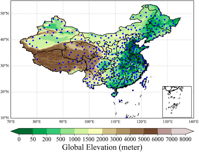
FIGURE 1. Spatial distribution of meteorological stations in China. The blue dots represent the stations.

FIGURE 2

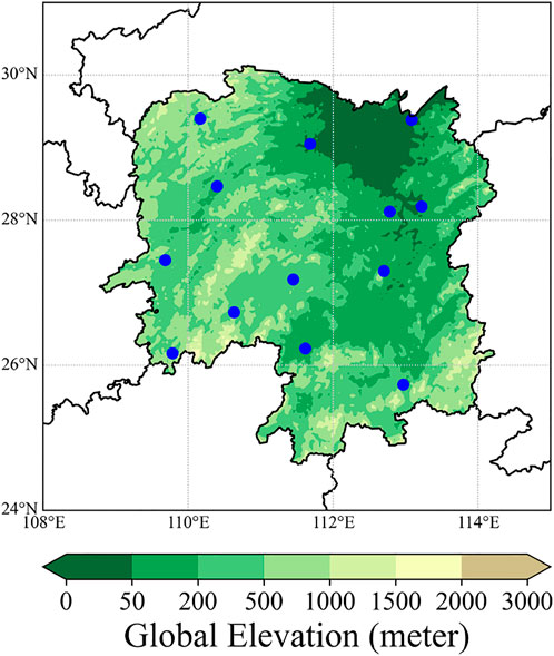
FIGURE 2. Spatial distribution of meteorological stations in Hunan Province.

2.2 Numerical weather prediction data

NWP is a quantitative and objective forecasting approach. Under certain initial and boundary conditions, NWP predicts the state of atmospheric motion for a specific period in the future by solving the hydrodynamics and thermodynamics equations, which explain the weather evolution process. Owing to the discretization of numerical calculation, the numerical weather forecast data are grid point data and it is challenging to precisely generate the atmospheric state for nongrid points. The elements of NWP comprise temperature, humidity, snowfall depth, total cloud cover, etc. NWP can generate the atmospheric state for a certain time in the future, and we assume that the forecast time series length is T. At the same time, the NWP data also have time intervals. If the time interval is 3 h, the maximum time limit of each forecast is 3*T. We record forecast data as p

$P={\left\{p_{n^{\prime },w\times h}^{l^{\prime }}\right\}}_{n^{\prime }=\mathrm{1,2},\dots ,N^{\prime },w=\mathrm{1,2},\dots ,W,h=\mathrm{1,2},\dots ,H}^{l^{\prime }=\mathrm{1,2},\dots ,L^{\prime }}(2)$

where L′ denotes the length of the forecast time series, N′ denotes the number of meteorological elements, and W × H denotes the grid size of the forecast.

The National Centers for Environmental Prediction (NCEP) operational Global Forecast System (GFS) forecast grids are used as another part of the input in our study (National Centers for Environmental Prediction et al., 2015). The GFS data are presented on a 0.25 by 0.25 global latitude–longitude grid, which comprises time steps at a 3-h interval from 0 to 240 h and a 12-h interval from 240 to 384 h. Model forecast runs occur at 00, 06, 12, and 18 UTC every day. We selected data from January 15, 2015 to January 31, 2018, to construct the dataset. Because the forecast error increases with time, we select a forecast period of 72 h for each forecast event.

3 Methodology

3.1 Data preprocessing

3.1.1 Historical observation data

For each station, we use the historical station data of 72 h before the initial forecast time, including 2-m temperature, 2-m dewpoint temperature, air pressure, wind direction, and wind speed. We normalize each meteorological element using zero-mean normalization, which is a normalization approach employing mean and standard deviation, to enhance the convergence ability of the model. At each station, numerous meteorological elements are recorded. The model input considerably affects the performance of the model. Eliminating unnecessary input features can decrease the complexity of the model and avoid noise to a certain extent, making the model more effective (Chakraborty et al., 2017).To extract more appropriate meteorological elements as input features, we investigated the effect of various meteorological elements on forecast elements based on random forest. Random forest is an ensemble classifier, which is built randomly and contains several decision trees, and its output is evaluated using the votes of each tree (Rigatti, 2017). Random forest can be used for solving classification and regression problems. For a certain feature, random forest determines the importance of the feature by adding noise to the feature; the larger the loss of the model, the more critical the feature after the addition of noise. We take a meteorological element as the target and other meteorological elements as the input to investigate the importance of the input variable to the target variable. Taking the 2-m temperature as the target, the results are shown in Table 1.

TABLE 1

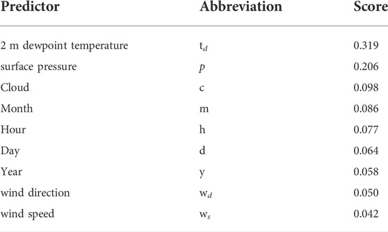
TABLE 1. Importance scores of variables.

3.1.2 Numerical weather prediction grid data

For NWP data, we selected the variables consistent with the forecast target elements. We did not select upper-air meteorological elements because the observation data obtained from stations are all near-surface data and the selected variables can well reveal the future state of the forecast target elements. We must extract the grid forecast data associated with each station. In this study, as shown in Figure 3, we extract the grid point data of 1° × 1° that is 9 × 9 with the station located at the center. Then, we use the CNN we constructed to propose the feature extraction that can extract more spatial distribution information of NWP and fully reflect the atmospheric state near the station. At the same time, zero-mean normalization is used to normalize the data.

FIGURE 3

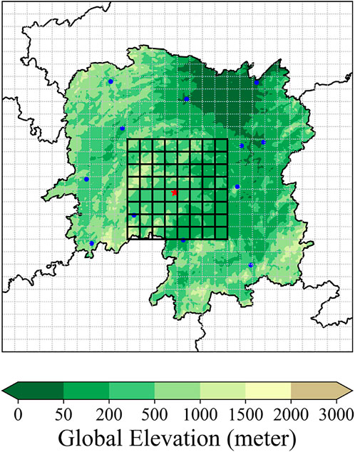
FIGURE 3. Extraction of GFS grid forecast data for a station.

3.2 Spatiotemporal convolution network

Based on the CNN and interactive convolution module, we built a spatiotemporal convolutional network (STCNet) to obtain the local weather forecast, as shown in Figure 4. The CNN is used to extract the spatial features of each forecast moment via two-dimensional convolution and convert the forecast data into time-series features. The interactive convolution module is used to process time series (Liu et al., 2021), which is done using one-dimensional convolution. First, for obtaining the historical station data, we use meteorological elements with high contributions as input using random forest; then, the input is processed by the interactive convolution module to generate features related to forecasting times. Second, for obtaining the forecast data, we use the CNN module to extract spatial features and use the interactive convolution module to update the time-series dimension for generating forecast features. These operations are presented as follows:

$X_f=ICM\left(X\right)and(3)$

$P_f=ICM\left(CNN\left(P\right)\right),(4)$

where X denotes the historical station data comprising meteorological elements with high contributions and p denotes the forecast data.

FIGURE 4

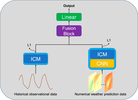
FIGURE 4. Overall structure of the spatiotemporal convolutional network.

For features X_f, P_f obtained from the two branches of our proposed model, we develop a gating module as a fusion module for feature fusion. We propose a gating unit K to weigh the contribution of various features, and feature weights are assigned using the gating unit. Finally, we fuse the features to generate the final prediction results using a fully-connected layer:

$K=sigmoid\left(W\ast X_f+W\ast P_f\right),(5)$

$Y=\left(1-K\right)\odot \left(W\ast X_f\right)+K\odot \left(W\ast P_f\right),and(6)$

$Y^{\prime }=Linear\left(Y\right),(7)$

where W denotes the one-dimensional convolution, K denotes the gating unit, and Y denotes the final fusion feature. Using temporal convolution, one-dimensional convolution can update the time-series relation and map features to hidden dimensions, whereas the fully-connected layer only implements linear mapping, so we choose one-dimensional convolution. sigmoid is the sigmoid function that maps the value to [0, 1], ⊙ is the Hadamard product, and Linear denotes the fully-connected layer.

We can convert the fusion process into the following formulas:

$Y=\left(W\ast X_f\right)+K\odot \left(W\ast P_f-W\ast X_f\right)and(8)$

$K=sigmoid\left(W\ast X_f+W\ast P_f\right).(9)$

The above shows that the fusion process is similar to the Kalman filter approach. We use the forecast feature X_f of the historical station data and feature P_f of the forecast data to generate the optimal estimate. The largest difference compared to the Kalman filter approach is that the gain matrix K is generated by learning.

3.3 Convolutional neural network

CNNs have always played a crucial role in computer vision (Chua, 1997). Convolution kernel has a local receptive field that can capture local features and conduct spatial downsampling to continuously extract more detailed features (O’Shea and Nash, 2015). For forecast grid data, we can perform convolutional operation to extract the meteorological element information from the forecast data. Traditionally, to generate the future atmospheric state of a certain station, we usually replace atmospheric state of the station with the adjacent grid data or use the adjacent grid data to interpolate to this station. In this study, by exploiting the local receptive field and spatial downsampling of convolution kernel, we build a module to extract feature information of forecast data near a station and match it with historical station data.

For a certain station, we selected a grid of 9 × 9, i.e., 1° × 1°, as the forecast information of meteorological elements near the station. Using the multilayer convolution operation, we constructed a CNN to extract features from the forecast grid data at each time t, then expand output into one-dimensional information, and finally pass through the fully-connected layer. The Relu activation was used between each layer, and the full structure of CNN is shown in Figure 5.

FIGURE 5

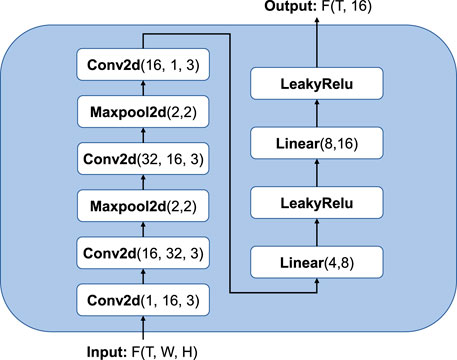
FIGURE 5. Structure of convolutional neural network. Conv2d represents the two-dimensional convolution, where the parameters represent the input channel, output channel, and convolution kernel size. The parameters of maxpool represent the pool size, and the parameters of linear represent the input and output dimensions.

3.4 Interactive convolution module

For realizing time-series forecasting tasks, recurrent neural networks are traditionally used (Shi et al., 2017; Li C. et al., 2019). A recurrent neural network is an iterated multistep evaluation approach that suffers from error accumulation. At the same time, gradient disappearance/explosion and information constraints also hinder the application efficiency if the model (Rangapuram et al., 2018). Therefore, we discard the recurrent neural network and use the interactive convolution module (ICM), which employs the convolution filter to capture the time-series changes in a short time (Liu et al., 2021).

The detailed structure of the ICM is shown in Figure 6. First, we downsample the sequence to generate two subsequences using odd–even splitting operation, and the downsampling process is recorded as

$X_{\mathit{odd}}=X_{2i-1},i=\mathrm{1,2},\dots ,L/2and(10)$

$X_{\mathit{even}}=X_{2i},i=\mathrm{1,2},\dots ,L/2,(11)$

where X_odd, X_even denotes the subsequences after downsampling. Downsampling the original sequence in the temporal dimension allows us to investigate dynamic information at different temporal resolutions.

FIGURE 6

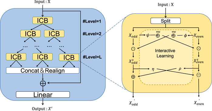
FIGURE 6. Structure of the interactive convolution module.

According to the ability of convolution to extract time information from time series, we develop a convolution extraction network, as shown in Figure 7, that comprises a series of one-dimensional convolutions, LeakyRelu activation, and a dropout layer. Time-series data represent continuous change within a short duration, which can be effectively captured by convolutions.

FIGURE 7

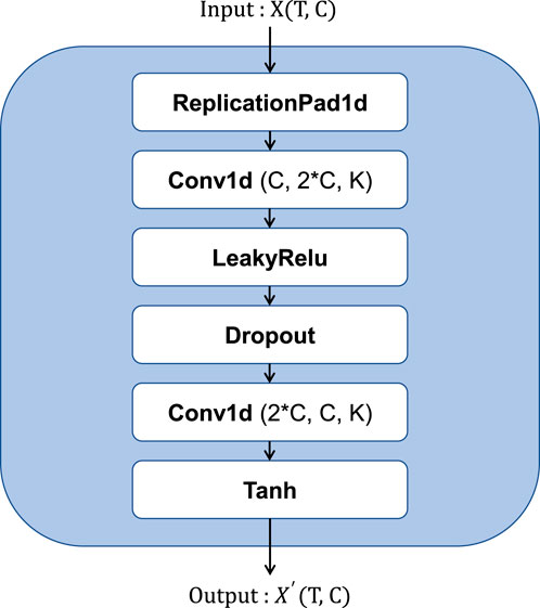
FIGURE 7. Structure of the convolution operation. Conv1d represents the one-dimensional convolution, where the parameters represent the input channel, output channel, and convolution kernel size.

To compensate for the information loss during downsampling, we use an interactive learning technique, which exchanges information between subsequences by learning affine transformation parameters. As shown on the right side of Figure 6, first, we transform X_odd and X_even extracted using the convolution extraction network into the form of exp, and then interact to X_even and X_odd with the element-wise product. Second, by repeating the convolution operation, $X_{\mathit{odd}}^s$ and $X_{\mathit{even}}^s$ are projected to the hidden state and then added to $X_{\mathit{odd}}^s$ and $X_{\mathit{even}}^s$. The detailed operations are as follows:

$X_{\mathit{odd}}^s=X_{\mathit{odd}}\ast \mathit{exp}\left(\varphi \left(X_{\mathit{even}}\right)\right),X_{\mathit{even}}^s=X_{\mathit{even}}\ast \mathit{exp}\left(\psi \left(X_{\mathit{odd}}\right)\right)and(12)$

$X_{\mathit{odd}}^{\prime }=X_{\mathit{odd}}^s+\rho \left(X_{\mathit{even}}^s\right),X_{\mathit{even}}^{\prime }=X_{\mathit{even}}^s+\eta \left(X_{\mathit{odd}}^s\right),(13)$

where ϕ, ψ, ρ, andη are all convolution extraction networks.

Finally, after repeated downsampling, the sequences of various time resolutions are updated via convolution feature extraction and interactive learning. Then we rearrange the subsequences by reversing the odd–even splitting operation and concatenate them into a new sequence representation, which is added to the original sequence through a residual connection (He et al., 2016). Further, the final output is generated through the connected layer. The specific operations are given as follows:

$X^{\prime }=\left(X_{\mathit{odd}}^{\prime },X_{\mathit{even}}^{\prime }\right)and(14)$

$X_{\mathit{out}}=Linear\left(X+X^{\prime }\right),(15)$

where X′ denotes the new sequence representation, X_out denotes the final output, and Linear represents the fully-connected layer.

3.5 Loss function

In this study, the historical station data and GFS forecast data are fused for local weather prediction and we process the two types of data separately. Further, we build the loss function based on intermediate supervision (Bai et al., 2018). In addition to supervising the final output results of the model, we supervise the two intermediate processing results of historical station data and GFS forecast data. The loss function is specifically expressed as follows:

$L=\alpha L_1\left(p_{\mathit{obs}}-p_{\mathit{true}}\right)+\beta L_1\left(p_{\mathit{gfs}}-p_{\mathit{true}}\right)+L_1\left(p-p_{\mathit{true}}\right),(16)$

where L₁ () denotes the Loss1 loss function and p_obs and p_true denote the intermediate processing results of historical station data and GFS forecast data, respectively, which are mapped from high-dimensional space to one-dimensional space using linear mapping. αandβ represent the trade-off parameters for various losses, we set both of them to 0.2.

4 Experiment

4.1 Data split

Since the forecast error increases with time, the longer the forecast period, the larger the error. For each forecast result, we only use the first 24 time values of forecast data as the input of NWP data and at the same time, use the 72 time values of historical station data before the start forecast time as another part of the input to build a sample. The next 72-h historical station data after start forecast time is used as ground truth. At the same time, we have selected 11 stations and we can get 48 samples per day. We have generated 50,000 samples in total. Specifically, the data from January 15, 2015 to November 30, 2016 are used as the training set, the data from December 1, 2016 to June 30, 2017 are used as the validation set, and the data from July 1 2017 to January 31 2018 are used as the test set. Finally, we divide the data set into the sets of training, validation, and test by time with a ratio of 6:2:2.

4.2 Evaluation indicators

To compute and estimate the performance of the various approaches, we used RMSE, mean absolute error (MAE), and accuracy (Acc). The RMSE is a common indicator for estimating regression problems, and MAE can be used to evaluate the deviation of the predicted value from the actual value. For a certain meteorological element p, because the total forecast time is T = 24, $P\in {\mathbb{R}}^{T\times 1}$ is a one-dimensional vector; therefore, RMSE and MAE are defined as

$RMSE=\sqrt{\frac{1}{N}\sum _1^N{\frac{1}{T}\left({\mathbf{P}}_{\mathit{pre}}^n-{\mathbf{P}}_{\mathit{true}}^n\right)}^{\text{t}}\left({\mathbf{P}}_{\mathit{pre}}^n-{\mathbf{P}}_{\mathit{true}}^n\right)}and(17)$

$MAE=\frac{1}{N}\sum _1^N\frac{1}{T}|{\mathbf{P}}_{\mathit{pre}}^n-{\mathbf{P}}_{\mathit{true}}^n|,(18)$

where P_pre denotes the prediction finding vector, P_true represents the true value vector, t is the matrix transpose notation, N denotes the total number of samples, and T represents the total forecast time.

Accuracy is a metric used for classification tasks. For regression tasks, we can convert the evaluation into a binary classification problem by setting a threshold. We set the threshold to σ, positive samples represent |P_pre − P_true|<σ, denoted as N_P, and negative samples represent |P_pre − P_true|≥ σ, denoted as N_G; therefore, the accuracy is expressed as

$ACC=\frac{N_P}{N_G+N_P}\times 100\%.(19)$

For various meteorological elements, the threshold σ has various values. According to (Li H. et al., 2019; Chen et al., 2020), σ is set to 2 °C to evaluate the post-processing method for temperature forecasting. Accordingly, we set σ as 2 °C for temperature and dewpoint temperature experiments.

4.3 Baseline methods

To confirm the effectiveness and superiority of our model, we use various approaches to perform comparative experiments. First, we use the sequence-to-sequence model (Seq2Seq) for comparison. The Seq2Seq model is an encoder–decoder architecture widely used in natural language processing (Sutskever et al., 2014). Encoders and decoders are usually based on recurrent neural networks, which can be used to process time-series data. Therefore, the Seq2Seq model is widely used in meteorology for short-term precipitation forecasts (Zhang et al., 2021), other meteorological elements forecast, etc. (Geng et al., 2019) (Kong et al., 2022).

Second, we only use historical station data and forecast data, combined with the ICM, to build observation-based interactive convolution network (obs-CNet) and GFS-based interactive convolution network (gfs-CNet) for investigating the functions of two types of data for local weather prediction and the effectiveness of our proposed fusion module.

4.4 Training details

We select the Adam optimizer and set the initial learning rate to 1 × e⁻³. At the same time, we select an exponential learning rate decay technique to increase the stability of training and set gamma to 0.97 (You et al., 2019). The batch size is set to 64 and the loss function is set to L1 loss. All models are implemented based on PyTorch.

5 Results

5.1 Performance of the proposed model with respect to meteorological elements

We perform experiments for 2-m temperature prediction. Based on random forest, we chose the 2-m dewpoint temperature, surface pressure, and 2-m temperature. The performances of various approaches using the test set are presented in Table 2. This table shows that the MAE and RMSE of the GFS forecast data are the largest, the Acc is the smallest, indicating that the GFS forecast data have a large error, and all approaches have a certain enhancement compared with the GFS data. The local weather prediction based purely on historical station data is better than that based on GFS forecast data, but its performance is poor because there is no prior information on the future atmospheric state. Based only on GFS forecast data, good results can be obtained, which demonstrates that GFS forecast data play a crucial role in explaining future elements for local weather forecasting. By fusing the two types of data, we can generate local weather forecast from the historical station data under the future atmospheric state’s background to generate better results. The results based on the Seq2Seq model outperform the above approaches on all metrics. Further, our proposed model achieves the best results with the smallest values of MAE and RMSE and an accuracy of 80%.

TABLE 2

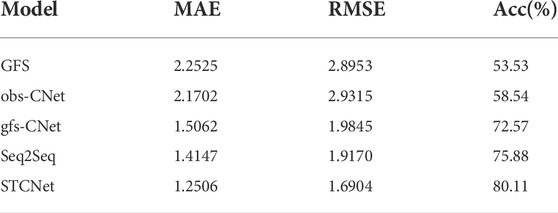
TABLE 2. Comparison of different methods regarding 2-m temperature forecasting.

To further investigate the performance of various approaches, Figure 8 shows the trend of RMSE and Acc with respect to the forecast time to reveal the detailed forecast performance of various approaches. In terms of Acc, the Acc of GFS forecast data is the worst, which has been retained at 0.55. The obs-CNet based on historical station data has a good initial prediction effect, but with an increase in the forecast time, the forecast accuracy rate reduces substantially. Compared with the original forecast data, the gfs-CNet based on forecast data has an enhancement of $>$0.2, indicating that the deep learning network plays a specific role in correcting the forecast errors. The fusion model of the historical station data and GFS forecast data exhibits the best performance. The Seq2Seq model can attain higher Acc than gfs-CNet, particularly at the initial stage of forecasting. Further, our proposed model attains the best performance, where the initial accuracy rate is retained above 0.9 and the final prediction accuracy rate can be maintained at ∼0.75, with a slower decay rate than the Seq2Seq model. Similar results are obtained regarding the RMSE. The forecast results of GFS are poor, while the error generated by the obs-CNet model increases rapidly with the forecast time. The Seq2Seq model and our proposed STCNet model perform well, where our proposed model exhibits the smallest error.

FIGURE 8

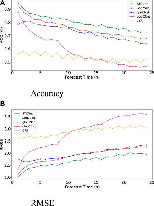
FIGURE 8. Accuracy and RMSE of different methods regarding 2-m temperature forecast with respect to forecast time.

Under the condition that the water vapor content in the air remains unchanged and the air pressure is constant, the temperature at which the air is cooled and reaches saturation is called the dewpoint temperature that can show the water vapor content of the atmosphere. We further investigated the performance of our proposed model and other approaches regarding 2-m dewpoint temperature forecasts. The 2-m temperature, surface pressure, and 2-m dewpoint temperature were chosen using random forecast. The performances of various approaches for the test set are shown in Table 3. At the same time, Figures 9A,B show the trend of RMSE and Acc of various models regarding the 2-m dewpoint temperature forecast with the forecast time, respectively. Similar the results of temperature forecasting, our proposed STCNet model shows the best performance, and its error has remained stable and minimal, not higher than 2 °C when the forecast time reaches 72 h. The proposed STCNet model can attain $>$90% Acc at the initial stage and $>$70% Acc with an increase in the forecast time.

TABLE 3

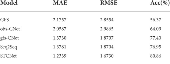
TABLE 3. Comparison of different methods regarding 2-m dewpoint temperature forecasting.

FIGURE 9

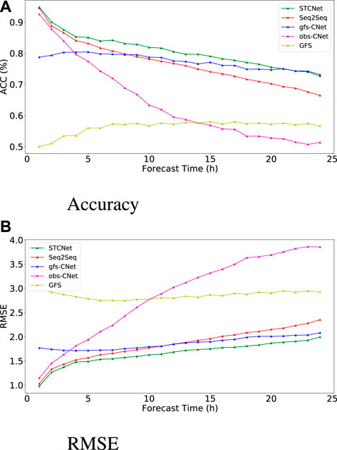
FIGURE 9. Accuracy and RMSE of different methods regarding 2-m dewpoint temperature forecast with respect to forecast time.

The comparison of different approaches above indicates the effectiveness and rationality of our proposed model. Figure 10 shows two cases of the variation trend of predicted and actual values in the forecast period. As shown in Figure 10A, when the future 2-m temperature exhibits periodic variation without abrupt changes, all approaches can predict the periodicity of future 2-m temperature. However, our proposed model is more accurate at extreme values in future 2-m temperature. As shown in Figure 10B, when the future temperature exhibits abrupt changes, obvious errors are observed in the GFS forecast data, and it is challenging to generate good results depending on the forecast data. It is also very difficult to predict sudden changes in future temperaature only depending on historical station data, especially when the forecast time is very far from the starting forecast time.Based on the fusion of historical station data and NWP data, we can obtain a more accurate trend of future atmospheric changes, which shows that the fusion method is appropriate and meaningful. Meanwhile, our proposed model can attain better result than the Seq2Seq model.

FIGURE 10

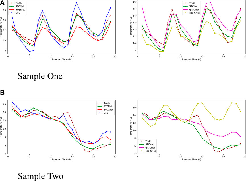
FIGURE 10. Comparison of the predicted and actual values using different methods.

5.2 Evaluation of model performance on different months and stations

Owing to the nonlinearity of atmospheric motion and the influence of various weather processes, the weather forecast results have differences in time evolution and spatial distribution (Dirren et al., 2003). Therefore, to fully evaluate different approaches, we performed comparative experiments for several months and at different stations. Additionally, we performed a corresponding study on the 2-m temperature prediction.

The RMSE of different approaches in different months is shown in Figure 11A. The obs-CNet model is better than the GFS forecast data in several months but substantially worse than the GFS forecast data in some months. The gfs-CNet model shows a considerable improvement over the GFS forecast data, and error is even reduced by half in June, July, and August. Further, our proposed STCNet model shows the best performance and better stability than other models, particularly in the second half of the year, indicating that seasonal changes have little influence on our model. Figure 11B shows the performances of models regarding RMSE at various stations; our proposed model consistently exhibits the best performance among all the stations while the RMSE does not vary extensively. This shows that our model can be applied to many stations at the same time, implying that our model has strong robustness and can complete the forecast at many stations at the same time, thus saving computing resources.

FIGURE 11

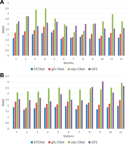
FIGURE 11. RMSEs of different methods for 2-m temperature forecasting in different months and at different stations.

5.3 Hourly forecast based on 3 h interval forecast data

Owing to the consumption of computing resources and a large storage capacity, it is challenging to generate detailed forecast data in time and space, which is also the reason why it is difficult to generate local weather forecasts within short time intervals. Thus, based on the GFS forecast data with an interval of 3 h, combined with the hourly historical station data, we completed the hourly local weather forecast for the furure 72-h to investigate the suitability of increasing the temporal and spatial resolutions of the forecast data. Because each output of a recurrent neural network corresponds to an input, it is challenging for a Seq2Seq model to achieve this task (Yin et al., 2017). Our proposed model is based on hybrid convolution, where one-dimensional convolution is used to process the time series; therefore, it is competent for this task.

Based on hourly historical station observations and GFS forecast data at 3-h interval, we have completed the local weather forecast for the future 72-h at 1-h interval. We completed investigations regarding 2-m temperature prediction using the STCNet model and obs-CNet model, and the performance for the test set is shown in Table 4. The table shows that the GFS forecast data have considerably improved the hourly temperature forecast. Although the time resolution is lower than the forecast demand, it can still offer future weather background information. At the same time, the results of our proposed model show an improvement in the temporal resolution and realize remarkable hourly local weather prediction. Compared with the 3-h interval forecast of STCNet model, the RMSE of local weather forecast at 1-h interval is increased only by 0.09, while the accuracy rate is only reduced by 2.2%, showing that our proposed model can complete the high-frequency forecast of the local weather when the temporal and spatial resolutions of the forecast data are inadequate.

TABLE 4

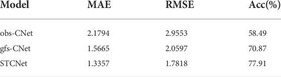
TABLE 4. Comparison of different methods regarding hourly 2-m temperature forecasting.

Figure 12 shows the variation of the predicted and true values in the hourly temperature forecast. The two forecast results reveal that our model not only captures the periodicity of the temperature changes but also attains more precise results, particularly around extreme values. In case of an abrupt temperature change (as shown in Figure 12B), the STCNet model can capture the change well, generating results consistent with the real change trend.

FIGURE 12

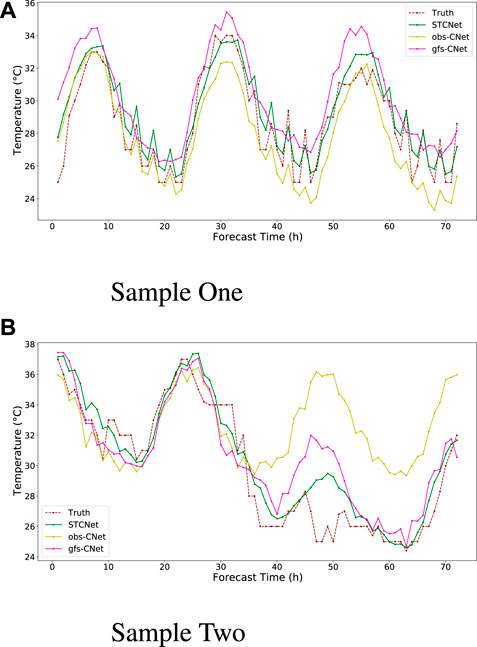
FIGURE 12. Comparison of the forecast and actual values with respect to hourly 2-m temperature forecasting.

6 Conclusion

In this study, we propose a deep learning model STCNet based on spatiotemporal modeling to achieve local weather prediction. Because the recurrent neural network is influenced by the accumulation of errors and faces a gradient disappearance/explosion challenge, we discard the traditional recurrent neural network and select the convolution networks for local weather prediction task. Through the extraction of spatial information using two-dimensional convolutions and the capture of time series via one-dimensional convolutions, we build a convolution-based spatiotemporal model. The main contributions of our study are as follows. 1. We have achieved the usage and fusion of multiple data. A large difference exists between historical station data and forecast data. The former present the historical information of a single station, and the latter comprise the future grid point information in a specific range of area. The successful fusion provides good local weather forecast results. 2. We experimented on many stations simultaneously, which shows that our model can be used to process data from multiple stations simultaneously and exhibits high robustness. 3. Based on the 3-h forecast data, we can also complete the hourly local weather forecast. Under the spatial and temporal resolution limitations of forecast data, we can enhance the temporal resolution and achieve the local weather forecast that fully makes up for the errors and low resolution of NWP model.

To fully confirm the forecasting ability of our proposed model, we performed 72-h meteorological element forecasts at 11 stations. Simultaneously, we compared the performance of our model with those of the Seq2Seq, obs-CNet, and gfs-CNet models. Additionally, we determined the influence of historical station data and GFS forecast data on forecasting. Using the 2-m temperature forecast as an example, our experiments demonstrate that the proposed model is superior to the Seq2Seq model, and the optimal forecast results can be generated based on the fusion of historical station data and GFS forecast data. Then, the analysis of RMSE obtained using different methods for various months and stations shows that our proposed model is the most stable between various months and has the smallest error among all stations, indicating that our model can be applied to various stations and in different seasons. Finally, we made hour-by-hour forecasts based on GFS forecast data with an interval of 3 h. The results show that our model can still have small errors and high accuracy and the accuracy is only 2.2% lower than the 3-h forecast, indicating that our proposed model can make up for the inadequate spatial and temporal resolutions of NWP data.

Generally, our proposed model fully employs historical station data and NWP data for local weather prediction and at the same time makes up for the lack of temporal and spatial resolutions of GFS forecast data to generate more refined forecasts. In actual weather prediction, there will be a significant practical applications. In the future, we will complete multielement comprehensive forecasting based on multistation forecasting and enhance the forecasting influence for extreme events in the weather process.

Data availability statement

The data of meteorological stations comes from National Climatic Data Center (NCDC), which is affiliated to National Oceanic and Atmospheric Administration. The data is available from NCDC’s public FTP server (ftp://ftp.ncdc.noaa.gov/pub/data/noaa/isd-lite/). The GFS data is available from NCEP GFS 0.25 Degree Global Forecast Grids Historical Archive, as cited in National Centers for Environmental Prediction et al., 2015.

Author contributions

LX and JX contributed to conception and design of the study. JG organized the database. LZ performed the statistical analysis. LX wrote the first draft of the manuscript. LX, LZ, ZC, and JX(5th author) wrote sections of the manuscript. All authors contributed to manuscript revision, and they read and approved the submitted version.

Funding

This work was supported by the National Natural Science Foundation of China (Project No. 41975066).

Acknowledgments

We thank the three reviewers for their comments, which helped us improve the manuscript.

Conflict of interest

The authors declare that the research was conducted in the absence of any commercial or financial relationships that could be construed as a potential conflict of interest.

Publisher’s note

All claims expressed in this article are solely those of the authors and do not necessarily represent those of their affiliated organizations, or those of the publisher, the editors and the reviewers. Any product that may be evaluated in this article, or claim that may be made by its manufacturer, is not guaranteed or endorsed by the publisher.

References

Aryal, Y., and Zhu, J. (2021). Evaluating the performance of regional climate models to simulate the us drought and its connection with el nino southern oscillation. Theor. Appl. Climatol. 145, 1259–1273. doi:10.1007/s00704-021-03704-y

CrossRef Full Text | Google Scholar

Bai, S., Kolter, J. Z., and Koltun, V. (2018). Trellis networks for sequence modeling. arXiv preprint arXiv:1810.06682.

Google Scholar

Bjerknes, V. (1904). Das problem der wettervorhers-age, betrachtet vom standpunkte der mechanik und der physik. Meteor. Z. 21, 1–7.

Google Scholar

Chakraborty, S., Tomsett, R., Raghavendra, R., Harborne, D., Alzantot, M., Cerutti, F., et al. (2017). “Interpretability of deep learning models: A survey of results,” in 2017 IEEE smartworld, ubiquitous intelligence & computing, advanced & trusted computed, scalable computing & communications, cloud & big data computing, Internet of people and smart city innovation (smartworld/SCALCOM/UIC/ATC/CBDcom/IOP/SCI) (San Francisco, CA, USA: IEEE), 1–6.

Google Scholar

Charney, J. G., Fjörtoft, R., and Neumann, J. v. (1990). “Numerical integration of the barotropic vorticity equation,” in The atmosphere—a challenge (Berlin, Germany: Springer), 267–284.

CrossRef Full Text | Google Scholar

Chen, K., Wang, P., Yang, X., Zhang, N., and Wang, D. (2020). A model output deep learning method for grid temperature forecasts in tianjin area. Appl. Sci. 10, 5808. doi:10.3390/app10175808

CrossRef Full Text | Google Scholar

Chua, L. O. (1997). Cnn: A vision of complexity. Int. J. Bifurc. Chaos 7, 2219–2425. doi:10.1142/s0218127497001618

CrossRef Full Text | Google Scholar

Cifuentes, J., Marulanda, G., Bello, A., and Reneses, J. (2020). Air temperature forecasting using machine learning techniques: A review. Energies 13, 4215. doi:10.3390/en13164215

CrossRef Full Text | Google Scholar

Dirren, S., Didone, M., and Davies, H. (2003). Diagnosis of “forecast-analysis” differences of a weather prediction system. Geophys. Res. Lett. 30, 2003GL017986. doi:10.1029/2003gl017986

CrossRef Full Text | Google Scholar

Ehrendorfer, M. (1997). Vorhersage der Unsicherheit numerischer wetterprognosen: Eine übersicht. metz. 6, 147–183. doi:10.1127/metz/6/1997/147

CrossRef Full Text | Google Scholar

Feng, S., Hu, Q., and Qian, W. (2004). Quality control of daily meteorological data in China, 1951–2000: A new dataset. Int. J. Climatol. 24, 853–870. doi:10.1002/joc.1047

CrossRef Full Text | Google Scholar

Geng, Y.-a., Li, Q., Lin, T., Jiang, L., Xu, L., Zheng, D., et al. (2019). “Lightnet: A dual spatiotemporal encoder network model for lightning prediction,” in Proceedings of the 25th ACM SIGKDD international conference on knowledge discovery & data mining, 2439–2447.

Google Scholar

Glahn, B. (2014). Determining an optimal decay factor for bias-correcting mos temperature and dewpoint forecasts. Weather Forecast. 29, 1076–1090. doi:10.1175/waf-d-13-00123.1

CrossRef Full Text | Google Scholar

Grönquist, P., Yao, C., Ben-Nun, T., Dryden, N., Dueben, P., Li, S., et al. (2021). Deep learning for post-processing ensemble weather forecasts. Phil. Trans. R. Soc. A 379, 20200092. doi:10.1098/rsta.2020.0092

CrossRef Full Text | Google Scholar

He, K., Zhang, X., Ren, S., and Sun, J. (2016). “Deep residual learning for image recognition,” in Proceedings of the IEEE conference on computer vision and pattern recognition, 770–778.

CrossRef Full Text | Google Scholar

Kong, W., Li, H., Yu, C., Xia, J., Kang, Y., and Zhang, P. (2022). A deep spatio-temporal forecasting model for multi-site weather prediction post-processing. Commun. Comput. Phys. 31, 131–153. doi:10.4208/cicp.oa-2020-0158

CrossRef Full Text | Google Scholar

Li, C., Zhang, Y., and Zhao, G. (2019a). “Deep learning with long short-term memory networks for air temperature predictions,” in 2019 International Conference on Artificial Intelligence and Advanced Manufacturing (AIAM) (Dublin, Ireland: IEEE), 243–249.

CrossRef Full Text | Google Scholar

Li, H., Yu, C., Xia, J., Wang, Y., Zhu, J., and Zhang, P. (2019b). A model output machine learning method for grid temperature forecasts in the beijing area. Adv. Atmos. Sci. 36, 1156–1170. doi:10.1007/s00376-019-9023-z

CrossRef Full Text | Google Scholar

Lin, H., Gao, Z., Xu, Y., Wu, L., Li, L., and Li, S. Z. (2022). Conditional local convolution for spatio-temporal meteorological forecasting.

Google Scholar

Liu, M., Zeng, A., Xu, Z., Lai, Q., and Xu, Q. (2021). Time series is a special sequence: Forecasting with sample convolution and interaction. arXiv preprint arXiv:2106.09305.

Google Scholar

[Dataset] National Centers for Environmental Prediction,National Weather Service,NOAA, andU.S. Department of Commerce (2015). Ncep gfs 0.25 degree global forecast grids historical archive. College Park, Maryland: National Centers for Environmental Prediction.

Google Scholar

Nerini, D., Foresti, L., Leuenberger, D., Robert, S., and Germann, U. (2019). A reduced-space ensemble kalman filter approach for flow-dependent integration of radar extrapolation nowcasts and nwp precipitation ensembles. Mon. Weather Rev. 147, 987–1006. doi:10.1175/mwr-d-18-0258.1

CrossRef Full Text | Google Scholar

O’Shea, K., and Nash, R. (2015). An introduction to convolutional neural networks. arXiv preprint arXiv:1511.08458.

Google Scholar

Peng, X., Che, Y., and Chang, J. (2014). “Observational calibration of numerical weather prediction with anomaly integration,” in EGU General Assembly Conference Abstracts, 5026.

Google Scholar

Qishu, W., Mei, H., Hong, G., and Tonghua, S. (2016). The optimal training period scheme of mos temperature forecast. 应用气象学报 27, 426–434.

Google Scholar

Rangapuram, S. S., Seeger, M. W., Gasthaus, J., Stella, L., Wang, Y., and Januschowski, T. (2018). Deep state space models for time series forecasting. Adv. neural Inf. Process. Syst. 31.

Google Scholar

Reichle, R. H. (2008). Data assimilation methods in the Earth sciences. Adv. water Resour. 31, 1411–1418. doi:10.1016/j.advwatres.2008.01.001

CrossRef Full Text | Google Scholar

Richardson, L. F. (2007). Weather prediction by numerical process. Cambridge: Cambridge University Press.

Google Scholar

Rigatti, S. J. (2017). Random forest. J. Insur. Med. 47, 31–39. doi:10.17849/insm-47-01-31-39.1

PubMed Abstract | CrossRef Full Text | Google Scholar

Roy, D. S. (2020). Forecasting the air temperature at a weather station using deep neural networks. Procedia Comput. Sci. 178, 38–46. doi:10.1016/j.procs.2020.11.005

CrossRef Full Text | Google Scholar

Shi, X., Chen, Z., Wang, H., Yeung, D.-Y., Wong, W.-K., and Woo, W.-c. (2015). Convolutional lstm network: A machine learning approach for precipitation nowcasting. Adv. neural Inf. Process. Syst. 28.

Google Scholar

Shi, X., Gao, Z., Lausen, L., Wang, H., Yeung, D.-Y., Wong, W. K., et al. (2017). Deep learning for precipitation nowcasting: A benchmark and a new model. Adv. neural Inf. Process. Syst. 30.

PubMed Abstract | Google Scholar

Sutskever, I., Vinyals, O., and Le, Q. V. (2014). Sequence to sequence learning with neural networks. Adv. neural Inf. Process. Syst. 27.

Google Scholar

Villén-Peréz, S., Heikkinen, J., Salemaa, M., and Mäkipää, R. (2020). Global warming will affect the maximum potential abundance of boreal plant species. Ecography 43, 801–811. doi:10.1111/ecog.04720

CrossRef Full Text | Google Scholar

Wang, B., Zou, X., and Zhu, J. (2000). Data assimilation and its applications. Proc. Natl. Acad. Sci. U. S. A. 97, 11143–11144. doi:10.1073/pnas.97.21.11143

PubMed Abstract | CrossRef Full Text | Google Scholar

Yin, W., Kann, K., Yu, M., and Schütze, H. (2017). Comparative study of cnn and rnn for natural language processing. arXiv preprint arXiv:1702.01923.

Google Scholar

You, K., Long, M., Wang, J., and Jordan, M. I. (2019). How does learning rate decay help modern neural networks? arXiv preprint arXiv:1908.01878.

Google Scholar

Yu, X., Shi, S., and Xu, L. (2021). A spatial–temporal graph attention network approach for air temperature forecasting. Appl. Soft Comput. 113, 107888. doi:10.1016/j.asoc.2021.107888

CrossRef Full Text | Google Scholar

Zhang, F., Wang, X., and Guan, J. (2021). A novel multi-input multi-output recurrent neural network based on multimodal fusion and spatiotemporal prediction for 0–4 hour precipitation nowcasting. Atmosphere 12, 1596. doi:10.3390/atmos12121596

CrossRef Full Text | Google Scholar

Zhu, Y. (2005). Ensemble forecast: A new approach to uncertainty and predictability. Adv. Atmos. Sci. 22, 781–788. doi:10.1007/bf02918678

CrossRef Full Text | Google Scholar