Slope stability prediction based on adaptive CE factor quantum behaved particle swarm optimization-least-square support vector machine

Since the prediction of slope stability is affected by the combination of geological and engineering factors with uncertainties such as randomness, vagueness and variability, the traditional qualitative and quantitative analysis cannot match the recent requirements to judge them accurately. In this study, we expect that the adaptive CE factor quantum behaved particle swarm optimization (ACE-QPSO) and least-square support vector machine (LSSVM) can improve the prediction accuracy of slope stability. To ensure the global search capability of the algorithm, we introduced three classical benchmark functions to test the performance of ACE-QPSO, quantum behaved particle swarm optimization (QPSO), and the adaptive dynamic inertia weight particle swarm optimization (IPSO). The results show that the ACE-QPSO algorithm has a better global search capability. In order to evaluate the stability of the slope, we followed the actual project and research literature and selected the unit weight, slope angle, height, internal cohesion, internal friction angle and pore water pressure as the main indicators. To determine whether the algorithm is scientifically and practically feasible for slope deformation prediction, the ACE-QPSO-, QPSO-, IPSO-LSSVM and single least-square support vector machine algorithms were trained and tested based on a real case of slope project with six index factors as the input layer of the LSSVM model and the safety factor as the output layer of the model. The results show that the ACE-QPSO-LSSVM algorithm has a better model fit (R²=0.8030), minor prediction error (mean absolute error=0.0825, mean square error=0.0110) and faster convergence (second iteration), which support that the ACE-QPSO-LSSVM algorithm emthod is more feasible and efficient in predicting slope stability.

1 Introduction

In geotechnical engineering, slope stability analysis has been a significant research area. In China, nearly 800 people died or missed every year caused by slope instability, resulting in economic losses of more than 600 million dollars (Wang et al., 2022). Therefore, it is essential to perform slope stability analysis to ensure the reliability of slopes and the safety of people in the vicinity.

The study of slope stability was first initiated in Sweden in the 1920s, when engineer Fellenius proposed the slice method, following which many researchers at home and abroad focused on the problem of slope stability (Gasmo et al., 2000; Samui 2008; Zhang et al., 2017; Wang et al., 2019). Slope stability analysis methods can be divided into qualitative, quantitative, and non-deterministic methodologies (Yan 2017). Methods of quantitative analysis are mainly divided into geological history analysis methods, engineering geological analogy methods, and graphic methods (Gao 2014). The quantitative analysis method can be classified into two types: the limit equilibrium method and the numerical simulation method (Gao 2014), the non-deterministic method is mainly divided into fuzzy mathematical method, gray system theory method, artificial neural network method, genetic method, probabilistic analysis method, etc., (Chakraborty and Dey 2022). Among these methods, quantitative analysis cannot calculate the deformation of a rock mass, whereas deformation calculations can be crucial in some cases, and the qualitative analysis method has the problem of the dominance of human subjective factors, and people with different experiences will reach different conclusions with the same information.

Due to these limitations, traditional quantitative and qualitative analysis methods are unsuitable for many situations (Chakraborty and Dey 2022). Recent advances in science and technology have led to the widespread adoption of artificial intelligence technology in slope engineering because of its faster performance and greater accuracy (Jiang et al., 2018; Huang et al., 2019; Huang et al., 2020a; Chang et al., 2020; Chang et al., 2022). Slope stability prediction methods based on artificial neural network (ANN) (Sakellariou and Ferentinou 2005; Cho 2009) and support vector machine (SVM) (Samui 2008; Tan et al., 2011) have received extensive attention from researchers. Although ANN has successfully been applied to slope stability prediction research, it still suffers from certain disadvantages, such as over-fitting, slow convergence, and poor generalization performance (Gülcü 2022). Contrary to ANN, SVM in machine learning can overcome the disadvantages and is well accepted in several fields including geology (Huang et al., 2020b), geotechnical engineering (Huang et al., 2022a), environmental science (Huang et al., 2010), agronomy (Thanh Noi and Kappas 2017), bioscience, etc., (Mourao-Miranda et al., 2005).

The least-square support vector machine (LSSVM), an advanced version of the SVM, reduces the complexity of the optimization process and can quickly solve linear and non-linear multivariate calibration problems (Li and Tian 2016). Thus, LSSVM has excellent application potential in slope stability prediction research. In general, LSSVM has a high level of accuracy and generalization based on the choice of its regularization parameter $\left(\gamma \right)$ and squared bandwidth $\left({\delta }^2\right)$ (Samui and Kothari 2011). Nevertheless, the choice of traditional LSSVM on $\gamma$ and ${\delta }^2$ is not well suited for slope stability prediction research (Samui and Kothari 2011; Zeng et al., 2021).

To better select $\gamma$ and ${\delta }^2$ for high level performance of LSSVM, several heuristic algorithms (Yu 2012; Kamari et al., 2014; Li et al., 2018; Suarez-Leon et al., 2018) such as genetic algorithm (GA) (Wu 2011b; Atashrouz et al., 2016; Wen et al., 2017), particle swarm optimization (PSO) (Zhao and Yin 2009; Wu 2011a; Yu et al., 2016) have been applied to the optimal selection of parameters for LSSVM. These optimization algorithms are well-received by researchers because of their versatility, such as fast and high efficiency, effective escape from local optimal solutions, and balancing local and global search (Wang et al., 2010; Viswanathan and Samui 2016; Gedik 2018). GA is a search (optimality-seeking) algorithm with natural selection principles and natural genetic mechanisms. The population-based heuristic search technique known as PSO was created at the same time by Kennedy and Eberhart in response to their studies of the social interactions between flocks of fish and birds. PSO is easier to implement than GA and performs better in multivariate function optimization. Rapid convergence and the discovery of almost ideal solutions (Juang 2004; Panda and Padhy 2008; Duan et al., 2013; Li et al., 2015; Wu et al., 2015). Since 1995, many researchers have tried different performance optimizations for PSO (Fan 2002; Wang et al., 2017). In 2004, Sun et al. introduced the quantum theory to PSO, called Quantum-behaved particle swarm optimization (QPSO) (Xu 2004). Theoretically, the global search algorithm QPSO can ensure good optimal results in the search space. As opposed to PSO, the iterative equations of QPSO do not require the velocity vector of the particles. It requires fewer parameters to be adjusted, which can be implemented more easily. In addition, researchers have confirmed that QPSO has excellent properties such as better global search capability and faster computational speed compared to the standard PSO algorithm on some widely used benchmark functions (Jun et al., 2004; Xu 2004), and has good potential for the evaluation of slope stability.

In summary, to compensate for the shortcomings of the slow solution speed of SVM and the limited search space of PSO, which is easy to fall into local optimal solutions. In this paper, an improved QPSO-LSSVM algorithm is proposed by optimizing the LSSVM parameters with adaptive CE factor quantum-behaved particle swarm (ACE-QPSO) and applied to the stability prediction study of slopes, subsequently analyzing sample data and case predictions to determine whether the algorithm is scientifically and practically feasible for slope deformation prediction.

2 Methods

The rest of this paper is structured as follows: Section 2 introduces the algorithmic principles of SVM, single LSSVM, and PSO, QPSO. Section 3 presents the improved QPSO-LSSVM algorithm applied to slope stability prediction. Section 4 tests the performance of the ACE-QPSO, QPSO, and IPSO algorithms through three classic benchmark functions. Section 5 compares the improved QPSO-LSSVM algorithm, QPSO-LSSVM algorithm, PSO-LSSVM, and single LSSVM algorithms for prediction and analysis based on training and testing samples for slope stability prediction. At the end of this paper, Section 6 presents the research conclusions. The modeling flow chart of slope stability prediction based on ACE-QPSO-LSSVM is shown in Figure 1.

FIGURE 1

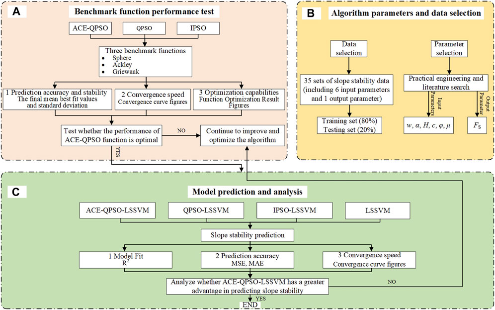
FIGURE 1. The modeling flow chart of slope stability prediction based on ACE-QPSO-LSSVM: (A) Benchmark function performance test, (B) Algorithm parameters and data selection, (C) Model prediction and analysis.

2.1 LSSVM algorithm

In 1995, Vapnik proposed the support vector machine (SVM) (Sain 1996), a supervised machine learning method for classification and regression. In recent years, SVM has received much attention due to its good classification performance and fault tolerance (Xuegong 2000; Huang et al., 2022b). Given a set of training samples $\left\{\left(x_i,y_i\right)|x_i\in R^n,i=\mathrm{1,2}\dots l\right\}$, where $x_i$ is a D-dimensional input vector and $y_i$ is an output indicator. The regression function can describe the non-linear relationship between the inputs and outputs:

$f\left(x\right)={\omega }^T\phi \left(x\right)+b(1)$

where $f\left(x\right)$ represents the predicted value, $\phi$ is the high-dimensional feature map, $\omega$ is the weight vector, and $b$ stands for the bias term. Considering that there is a fitting error, we can introduce slack variables ${\xi }_i\ge 0$ and ${\xi }_i^{*}\ge 0$. Therefore, we derive the following error minimization expression:

$MinJ\left(\omega ,\xi ,{\xi }^{*}\right)=\frac{1}{2}\left(\omega \cdot {\omega }^T\right)+c{\displaystyle \sum }_{i=1}^l\left({\xi }_i+{\xi }_i^{*}\right)(2)$

$\left\{\begin{array}{c}{y}_i-\omega \cdot \phi \left(x_i\right)-b\le \epsilon +{\xi }_i\\ \omega \cdot \phi \left(x_i\right)+b-y_i\le \epsilon +\xi \\ {\xi }_i,{\xi }_i^{*}\ge 0\end{array}\right.(3)$

In Eq. 2, $c$ is the penalty function. Then the constraint is expressed as follows. For Eq. 3, Suykens et al. proposed a least-square support vector machine (LSSVM) (Suykens and Vandewalle, 1999) based on regularization theory, which transforms the above equation into:

$MinJ\left(\omega ,e\right)=\frac{1}{2}{\omega }^T\omega +\frac{1}{2}c{\displaystyle \sum }_{i=1}^l{e}_i^2(4)$

The above equation is constrained by $y_i={\omega }^T\phi \left(x_i\right)+b+e_i,i=\mathrm{1,2},\dots ,N$, where $e_i\ge 0$ is a non-negative relaxation variable. Furthermore, the optimization problem is solved using the Lagrange method, which corresponds to the Lagrange function as the Eq. 5 where ${\alpha }_i$ is a Lagrange multiplier. Then taking partial derivatives of the Eq. 5 and by eliminating $\omega$ and $e_i$ (Espinoza et al., 2006) yields the following linear system as the Eq. 6 in which $K\left(x,x_i\right)=\phi \left(x\right)\phi {\left(x_i\right)}^T$ is the kernel function and satisfies Mercer’s condition. The mentioned regression function obtains as the Eq. 7 in which ${\alpha }_i$ and $b$ express the solution of the linear system shown in Eq. 5.

$L\left(\omega ,b,e,\alpha \right)=\frac{1}{2}{\omega }^T\omega +\frac{1}{2}c{\displaystyle \sum }_{i=1}^l{e}_i^2-{\displaystyle \sum }_{i=1}^l{\alpha }_i\left[{\omega }^T\phi \left(x_i\right)+b+e_i-y_i\right](5)$

$\left[\begin{array}{cccc}0& 1& \dots & 1\\ 1& K\left(x,x_i\right)+\frac{1}{c}& \dots & K\left(x,x_i\right)\\ ⋮& ⋮& \cdots & ⋮\\ 1& K\left(x,x_i\right)& \cdots & K\left(x,x_i\right)+\frac{1}{c}\end{array}\right]\left[\begin{array}{c}b\\ {\alpha }_1\\ ⋮\\ {\alpha }_l\end{array}\right]=\left[\begin{array}{c}0\\ y_1\\ ⋮\\ y_l\end{array}\right](6)$

$y\left(x\right)={\displaystyle \sum }_{i=1}^l{\alpha }_{i}K\left(x,x_i\right)+b(7)$

The main kernel functions used for LSSVM are the following options: linear kernel function, polynomial kernel function, radial basis function (RBF), and Sigmoid kernel function. Kang et al. (Kang et al., 2016) have shown that by using different kernel functions in LSSVM for slope stability analysis studies, RBF significantly outperforms other kernel functions. Therefore, in this study, the RBF kernel function is used and expressed as the Eq. 8 where $\sigma$ is the width of the RBF that influences how the RBF’s inputs are scaled.

$K\left(x,x_i\right)=\exp \left(-\frac{{‖x-x_i‖}^2}{2{\sigma }^2}\right)(8)$

2.2 QPSO algorithm

2.2.1 Adaptive dynamic inertia weight particle swarm optimization (IPSO)

The PSO algorithm is a population-based heuristic search technique developed by James Kennedy and Russell Eberhart in 1995 by observing and studying the social behavior of flocks of birds and fish. Particles’ position and velocity are updated by Eqs 9, 10 in each step:

$X_i^{k+1}=X_i^k+V_i^{k+1}(9)$

$V_i^{k+1}=\omega V_i^k+c_1{r}_1\left(p_{best,i}^k-X_i^k\right)+c_2{r}_2\left(g_{best}^k-X_i^k\right)(10)$

In the above equation, $X_i^k$ denotes the N-dimensional vector of the particle $\left(i\right)$ at iteration $\left(k\right)$, $V^i$ denotes the velocity of the particle, $\omega$ denotes the inertia weight factor, $c_1,c_2$ denotes the learning factor, and $r_1,r_2$ denotes random functions in the range [0,1].

The inertia weight $\omega$ represents the effect of the velocity of the previous generation of particles on the velocity of the contemporary particles, or the degree of confidence the particles have in the current state of their own motion, and the particles move inertially based on their own velocity. Thus, PSO performance is governed by inertia weight $\omega$, which balances the population’s global and local development capabilities. Generally, in large problem spaces, to achieve a balance between search speed and search accuracy, algorithms are designed to have a high global search capability at an early stage to obtain a suitable seed, and a high local search capability at a later stage to improve convergence. Therefore, $\omega$ should not be a fixed constant (Ab Wahab et al., 2015). At present, the linear reduction is the most commonly used method for controlling $\omega$, but this method does not maintain a balance between global and local search (Bergh, F.V. and Engelbrecht 2004; Deng et al., 2017). In conjunction with the prediction object, therefore, we propose an adaptive dynamic change of inertia weights to adjust the value of $\omega$ to improve the performance further, as shown in Eq. 11, which is the adaptive dynamic inertia weight particle swarm optimization (IPSO).

$\omega ={\omega }_{\max }+\left({\omega }_{\max }-{\omega }_{\min }\right)\sin \left(\pi +\pi \times \frac{t}{2T}\right)(11)$

where ${\omega }_{\max }=0.9;{\omega }_{\min }=0.4$; $t$ is the current iteration number; and $T$ is the maximum iteration number.

2.2.2 Adaptive CE factor quantum-behaved particle swarm (ACE-QPSO)

As mentioned in introduction, two disadvantages of the PSO algorithm are its inability to guarantee the global optimal solution, and its poor local search capability, which results in poor search accuracy (Xinchao 2010). To solve this problem, Sun et al. developed and proposed the QPSO algorithm (Jun Sun 2004; Xu 2004), inspired by PSO and quantum mechanical trajectory analysis. Their iterative equation for particle movement is defined as follows:

$x_{i,j}\left(t+1\right)=p_{i,j}\left(t\right)+\alpha \cdot \left|mbes{t}_j\left(t\right)-x_{i,j}\left(t\right)\right|\cdot \ln \left(\frac{1}{u}\right)ifk\ge 0.5(12)$

$x_{i,j}\left(t+1\right)=p_{i,j}\left(t\right)-\alpha \cdot \left|mbes{t}_j\left(t\right)-x_{i,j}\left(t\right)\right|\cdot \ln \left(\frac{1}{u}\right)ifk<0.5(13)$

where,

$p_{i,j}\left(t\right)={\phi }_{i,j}\left(t\right)\cdot pbes{t}_{i,j}\left(t\right)+\left(1-{\phi }_{i,j}\left(t\right)\right)\cdot gbes{t}_j\left(t\right)(14)$

$mbes{t}_j\left(t\right)=\frac{1}{nPop}{\displaystyle \sum }_{i=1}^{nPop}pbes{t}_{i,j}\left(t\right)(15)$

From Eqs 12–15, $mbest$ is the average best position, one can obtain this by calculating the average of all the best positions ($pbest$) in the population; $k,u,\phi$ is the random functions uniformly distributed in the range [0,1]; and $\alpha$ parameter is the contraction-expansion coefficient (i.e., CE coefficient), which is the only parameter in the QPSO algorithm that can be adjusted to control the convergence rate of the algorithm. Usually, there are two main methods of controlling $\alpha$, one is to fix the value of $\alpha$ during the search period. In the previous research, it was noted that setting numbers in the range (0.5, 0.8) produces satisfactory results for most benchmark functions, and QPSO generally performs well when $\alpha$ =0.75 (Sun et al., 2011). However, the fixed value $\alpha$ is dependent on the population size and the number of iterations allowed. The other is to change the value of $\alpha$ by using a time-varying function expression. Research on QPSO has shown that non-linearly decreasing the value of $\alpha$ from ${\alpha }_1$ to ${\alpha }_0$ (${\alpha }_0<{\alpha }_1$) during the search process allows the QPSO algorithm to perform efficiently (He and Lu 2021; Lu and He 2021). In this paper, we combine the prediction objects and propose a method to adaptively change the CE coefficient (i.e., $\alpha$) to further improve the performance. A new equation is presented by the Eq. 16, which is the adaptive CE factor quantum-behaved particle swarm.

$\alpha ={\alpha }_{\max }-\left({\alpha }_{\max }-{\alpha }_{\min }\right)\frac{f\left(x\right)-f_w}{f_b-f_w}(16)$

where ${\alpha }_{\max },{\alpha }_{\min }$ refer to maximum and minimum values of $\alpha$, respectively; $f\left(x\right)$ is the current fitness of the particle; $f_w$ is the fitness of the worst particle in the population; and $f_b$ represents the best fitness in the population.

2.3 ACE-QPSO-LSSVM algorithm

The parameter regularization parameter ($\gamma$) and squared bandwidth (${\delta }^2$) optimization problem of LSSVM is usually converted into a parameter estimation problem for multiple linear regression functions (Xue 2017). Moreover, QPSO, as a global optimization algorithm, can quickly optimize these two parameters and iteratively change the values of $\gamma$ and ${\delta }^2$ to improve the prediction accuracy of LSSVM. Therefore, this paper proposes an ACE-QPSO-LSSVM algorithm to predict slope stability and uses performance metrics to evaluate its performance. And the performance metrics considered are defined as follows (Kang et al., 2016; Chen 2019).

${\mathrm{R}}^2=1-\frac{{{\displaystyle \sum }_i\left({\widehat{y}}_i-y_i\right)}^2}{{\displaystyle \sum }_i{\left({\overline{y}}_i-y_i\right)}^2}(17)$

$\mathrm{M}\mathrm{A}\mathrm{E}=\frac{1}{n}{\displaystyle \sum }_{i=1}^n\left|y_i-{\widehat{y}}_i\right|(18)$

$\mathrm{M}\mathrm{S}\mathrm{E}=\frac{1}{n}{\displaystyle \sum }_{i=1}^n{\left(y_i-{\widehat{y}}_i\right)}^2(19)$

Where $y_i$ denotes the measured value, ${\widehat{y}}_i$ indicates the predicted value, ${\overline{y}}_i$ denotes the mean value, and $n$ is the number of samples used for training. Apparently, as the coefficient of determination (R²) grows, the mean absolute error (MAE) and mean square error (MSE) values decrease, the algorithm prediction accuracy increases, and vice versa.

Then the main steps in this paper to implement the ACE-QPSO optimized LSSVM algorithm based on Python are as follows.

Step1:. Divide the prediction dataset into training and testing samples and normalize it. The standardized formula is presented by the follows:

$X_{norm}=\frac{X-X_{\min }}{X_{\max }-X_{\min }}(20)$

in Eq. 20, $X_{\min },X_{\max }$ are the minimum and maximum values in the dataset, respectively; $X_{norm}$ is the value after the normalization process; $X$ is the original sample values.

Step2:. Initialize the parameters of the QPSO algorithm, including the particle swarm size $S$, particle dimension $D$, the maximum number of iterations $T_{\max }$, the CE control coefficient $\alpha$, and the range of the parameters.

Step3:. Calculate the fitness of each particle by Eq. 19.

Step4:. Use Eq. 14 to calculate $p_{i,j}\left(t\right)$ and Eq. 15 to calculate the mean personal best position of the population $mbest$.

Step5:. Compare each particle’s fitness and corresponding parameters with their best known position $pbest$. If the current particle’s fitness and related parameters are better than $pbest$, update $pbest$ and fix the particle position parameter values between the minimum and maximum positions. On the contrary, not update $pbest$.

Step6:. Compare $pbest$ with the entire swarm’s best known position $gbest$. If $pbest$ is smaller than $gbest$, update $gbest$ fitness as well as particle swarm. On the contrary, not update $gbest$.

Step7:. Repeat Step3 to Step6 until the iteration termination condition is met. Output the parameters $\gamma$ and $\delta$ at this point, and use the parameters to train and predict the least squares support vector machine LSSVM regression model.The flow chart of the ACE-QPSO optimized LSSVM algorithm for slope stability prediction analysis is shown in Figure 2.

FIGURE 2

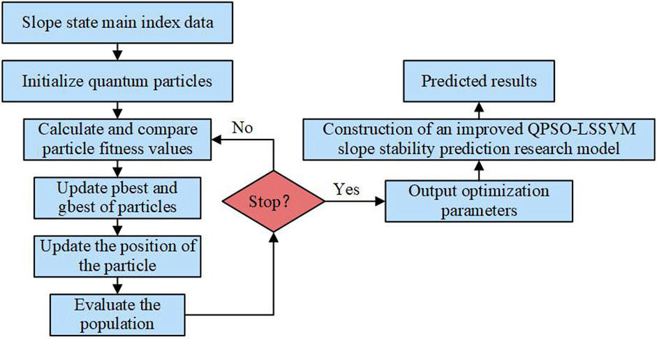
FIGURE 2. Flow chart of ACE-QPSO optimized LSSVM algorithm.

2.4 Performance measurement

To better compare the performance of the ACE-QPSO-LSSVM algorithm with the QPSO-LSSVM, IPSO-LSSVM algorithm, and as a preparation for the case study below. In this paper, each algorithm’s global optimal search ability is tested by the benchmark function. Then, ACE-QPSO, QPSO and IPSO will be tested for their respective optimization efficiency by three classical benchmark functions (Table 1), respectively.

TABLE 1

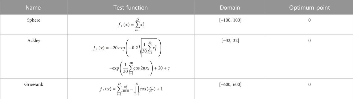
TABLE 1. Three benchmark functions.

To avoid the contingency of algorithm search, each algorithm was set to run 50 times for each test function with 200 iterations each. The final mean best fit values (Mean) and standard deviation (St Dev) were obtained as shown in Table 2, while the convergence curves and function result plots of their best fit values are shown in Figures 3, 4. Combined with Table 2, it can be seen that the mean best fitness value and standard deviation of ACE-QPSO are better than QPSO and IPSO, with the best convergence accuracy under the tests of three different benchmark functions. Meanwhile, it can be seen from Figure 3 that, overall, ACE-QPSO has faster convergence and higher optimization efficiency compared with QPSO and IPSO, and can obtain the best fitness value in a relatively short period. This indicates that ACE-QPSO has better performance in finding the optimal.

TABLE 2

TABLE 2. Comparison of the results of each algorithm.

FIGURE 3

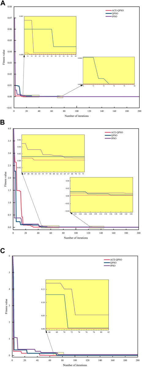
FIGURE 3. The convergence curves of each algorithm on the three benchmark functions of (A)–(C), respectively: (A) Sphere function; (B) Ackley function; (C) Griewank function.

FIGURE 4

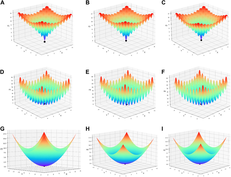
FIGURE 4. Optimization search results for each function: (A) IPSO&Ackley, (B) IPSO&Griewank, (C) IPSO&Sphere, (D) QPSO&Ackley, (E) QPSO&Griewank, (F) QPSO&Sphere, (G)ACE-QPSO&Ackley, (H) ACE-QPSO&Griewank, (I) ACE-QPSO&Sphere.

In Figures 4A–I represents the function images and the best-seeking results of IPSO, QPSO, and ACE-QPSO on the three benchmark functions of Ackley, Griewank, and Sphere, in turn. As can be seen in Figure 4, all the above algorithms are detected as globally converged, but the optimal positions in (a)–(c) are (0.008, 0.444), (−0.005, −0.006), (−0.0002, −0.0003), respectively; in (d)–(f) are (0.625, −0.007), (0.002 (0.001), (0.0004, 0.0006); and in the best positions of (g)–(i) (−0.512, −0.508), (−0.0005, 7.7 × 10⁻⁵), (1.2 × 10⁻⁵, 1.8 × 10⁻⁵), respectively. The comparison shows that the optimal solution coordinates obtained by ACE-QPSO under each benchmark function are closest to the global optimal solution coordinates, which indicates that ACE-QPSO has better global search capability.

3 Materials

3.1 Analysis and selection of factors influencing the stability of slopes

In practical projects, researchers classify slope stability into two categories: destructive slopes and stable slopes (Tien Bui et al., 2016; Zhang et al., 2021; Jiang et al., 2022). There are many factors that affect slope stability, including geomorphic conditions, stratigraphic lithology, geological structure, rock structure, and groundwater action, among others. Therefore, the selection of influencing factors is an essential prerequisite for evaluating the stability of slopes correctly. Among them, unit weight (w), slope angle (α), and height (H) are the main influencing factors of slope geometry, and slope stability decreases with increasing height, increasing slope angle, and decreasing weight (Zhou et al., 2019; Chen et al., 2021). In addition, it is known from the research of previous researchers (Cha and Kim 2011) that internal cohesion (c), internal friction angle (φ), and pore water pressure (μ) are also important factors affecting slope stability. Therefore, in this paper, the six factors of unit weight (w), slope angle (α), height (H), internal cohesion (c), internal friction angle (φ), and pore water pressure (μ) are selected as the leading indicators to evaluate the stability state of slopes.

3.2 Case data

In this study, 35 sets of slope stability data were collected from the data given by Keqiang He et al. (Keqiang He 2001), and the data set was randomly divided into 28 training samples and 7 testing samples (Table 3). As shown in Table 3, the input layer of the model includes six index parameters, namely unit weight(w), slope angle(α), height(H), internal cohesion (c), internal friction angle(φ), and pore water pressure(μ); the output layer is the safety factor, denoted by F_S.

TABLE 3

TABLE 3. Sample dataset.

4 Results

4.1 Parameter setting

This paper uses four algorithms, ACE-QPSO-LSSVM, QPSO-LSSVM, IPSO-LSSVM, and single LSSVM to train and predict the Section 3.2’s sample dataset. To better compare the prediction performance of each algorithm, for the first three algorithms, the number of particle swarms and algorithm iterations are 100 and 50, respectively. And the range of $\gamma ,\delta$ parameters is [0.001,100]. While single LSSVM traverses the debugging $\gamma ,\delta$ parameters through grid search, where $\delta$ ranges in [1,100] in 10 stepping cycles and $\gamma$ takes values from {0.001, 0.01, 0.1, 1, 5, 10} in sequential traversal cycles. Meanwhile, we use adaptive inertia weight (Eq. 11) for IPSO and make the learning factor c₁=c₂=2, while adaptive CE coefficient (Eq. 16) is used for ACE-QPSO.

4.2 Analysis of training performance results

The performance of each algorithm in training the samples is shown in Table 4 and Figure 5. Table 4 reflects the performance of the algorithm to train samples by listing the prediction values and MSE values obtained from the training samples of each algorithm. From Table 4, it is seen that ACE-QPSO-LSSVM performs the best in the training samples, and its MSE is the smallest among the four algorithms, only 0.0345, which is 80.21%, 85.25%, and 88.60% lower than QPSO-LSSVM, IPSO-LSSVM, and single LSSVM, respectively. Figure 5 then directly shows the comparison between the sample and predicted values after training the training set for each algorithm. From Figure 5, it is seen that, overall, the predicted values of ACE-QPSO-LSSVM are closer to the sample values and basically match the predicted trend, and its prediction effect is the most outstanding among the four algorithms, with a more stable and accurate prediction performance.

TABLE 4

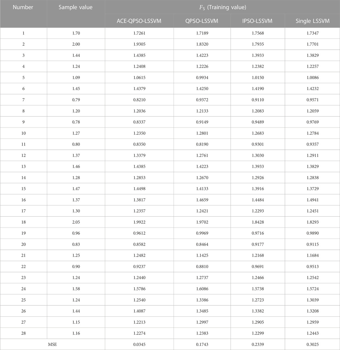
TABLE 4. Comparison between target and estimated values from each algorithm for the training samples.

FIGURE 5

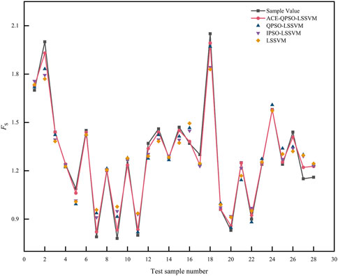
FIGURE 5. Comparison of the training results of each algorithm.

4.3 Analysis of convergence rate

The fitness curves of ACE-QPSO-LSSVM, QPSO-LSSVM, and IPSO-LSSVM throughout 50 iterations are shown in Figure 6.Combined with Figure 6, it is seen that all three algorithms can complete convergence by 50 iterations. However, compared with QPSO-LSSVM and IPSO-LSSVM, ACE-QPSO-LSSVM has the best convergence and a relatively higher speed, and it achieves convergence at the second iteration with the best fitness value of 0.0110. Thus, the ACE-QPSO-LSSVM algorithm with better convergence has tremendous potential and advantages for slope stability prediction research.

FIGURE 6

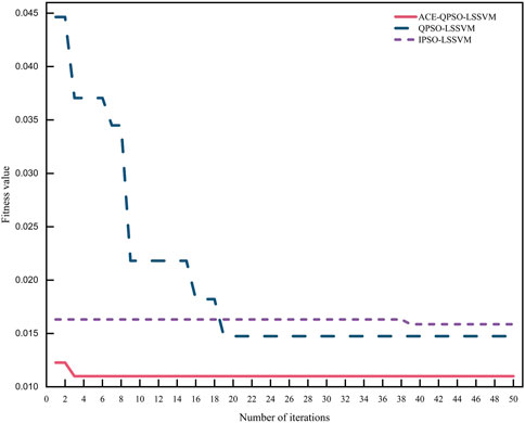
FIGURE 6. Fitness curve of each algorithm.

4.4 Analysis of prediction accuracy and model goodness of fit

The performance of each algorithm in the testing sample is shown in Table 5 and Figure 7. Then Table 5 reflects the ability of each algorithm to test samples by listing the prediction values and MSE values obtained after testing the samples. Combined with Table 5, it is evident that ACE-QPSO-LSSVM performs the best in the testing samples, and its MSE value is significantly lower than the other three algorithms at 0.0311, which is 69.84%, 71.98%, and 77.34% lower relative to QPSO-LSSVM, IPSO-LSSVM, and single LSSVM, respectively. Figure 7 directly shows the comparison between the sample values and the predicted values after the prediction of each algorithm for the testing set. From Figure 7, it is seen that the deviations between the predicted and sample values of the ACE-QPSO-LSSVM algorithm are minor, and its predicted values are the closest to the actual situation among the four algorithms, with the best prediction performance.

TABLE 5

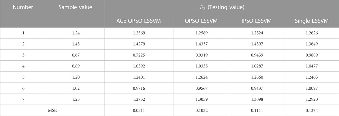
TABLE 5. Comparison between target and estimated values from each algorithm for the testing samples.

FIGURE 7

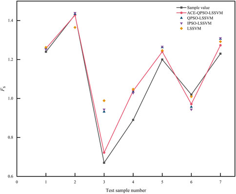
FIGURE 7. Comparison of the training results of each algorithm.

To avoid the chance of algorithm training and to ensure the scientific comparison of its performance, we independently repeated 50 times for each algorithm, and used the mean value to calculate the prediction results. Table 6 below shows the final estimated parameters obtained by each algorithm, and Table 7 compares the prediction performance of each algorithm under the three performance metrics of R², MAE, and MSE. Combined with Table 7, by comparing the performance metrics results of each algorithm, we found that the ACE-QPSO-LSSVM algorithm has a better fitting effect, and its R² value is significantly higher than the other three algorithms, which is 0.8030. In addition, the MAE and MSE values of ACE-QPSO-LSSVM are 0.0825 and 0.0110, respectively, which are smaller than the other three algorithms. It fully indicates that ACE-QPSO-LSSVM has a minor deviation between the predicted and actual values, with more accurate prediction performance.

TABLE 6

TABLE 6. Estimated parameters finally obtained by each algorithm.

TABLE 7

TABLE 7. Comparison of performance metrics for each algorithm.

In summary, the ACE-QPSO-LSSVM algorithm outperforms QPSO-LSSVM, IPSO-LSSVM, and single LSSVM in slope stability prediction with its better fit merit, more minor prediction error, and relatively higher speed, thus having good potential for application. For future work, the ACE-QPSO-LSSVM algorithm can be further explored and developed in terms of changing the form of the CE coefficient in the iterative process, optimizing the selection of model input parameters, as well as expanding and improving the sample data sets, which in turn can provide reference values for slope stability assessment and prediction research.

5 Conclusion

This paper proposed an improved algorithm for slope stability prediction based on ACE-QPSO optimized LSSVM. The method can dramatically improve the convergence speed and accuracy of the QPSO algorithm by adaptively improving the CE coefficient, then will provide better adaptation in shorter period. By verifying performance tests and case studies, the results supported that proposed ACE-QPSO has better optimal search capability and search efficiency in prediction of slope stability.

The case study results show that ACE-QPSO-LSSVM has a better model fit (R²=0.8030) and minor prediction error (MAE=0.0825, MSE=0.0110) and faster convergence (second iteration) compared with QPSO-LSSVM, IPSO-LSSVM and single LSSVM. In addition, ACE-QPSO-LSSVM shows better accuracy and stability than the other three algorithms under the benchmark function test.

Data availability statement

The original contributions presented in the study are included in the article/supplementary material, further inquiries can be directed to the corresponding author.

Author contributions

JY is responsible for all the tasks of this work.

Funding

This work was supported by National College Student Innovation and Entrepreneurship Training Program (202110635047X).

Conflict of interest

The authors declare that the research was conducted in the absence of any commercial or financial relationships that could be construed as a potential conflict of interest.

Publisher’s note

All claims expressed in this article are solely those of the authors and do not necessarily represent those of their affiliated organizations, or those of the publisher, the editors and the reviewers. Any product that may be evaluated in this article, or claim that may be made by its manufacturer, is not guaranteed or endorsed by the publisher.

References

Ab Wahab, M. N., Nefti-Meziani, S., and Atyabi, A. (2015). A comprehensive review of swarm optimization algorithms. PLoS One 10, e0122827. doi:10.1371/journal.pone.0122827

PubMed Abstract | CrossRef Full Text | Google Scholar

Atashrouz, S., Mirshekar, H., Hemmati-Sarapardeh, A., Moraveji, M. K., and Nasernejad, B. (2016). Implementation of soft computing approaches for prediction of physicochemical properties of ionic liquid mixtures. Korean J. Chem. Eng. 34, 425–439. doi:10.1007/s11814-016-0271-7

CrossRef Full Text | Google Scholar

Bergh, F. V., and Engelbrecht, A. P. (2004). A Cooperative approach to particle swarm optimization. IEEE Trans. Evol. Comput. 8, 225–239. doi:10.1109/tevc.2004.826069

CrossRef Full Text | Google Scholar

Cha, K.-S., and Kim, T.-H. (2011). Evaluation of slope stability with topography and slope stability analysis method. KSCE J. Civ. Eng. 15, 251–256. doi:10.1007/s12205-011-0930-5

CrossRef Full Text | Google Scholar

Chakraborty, R., and Dey, A. (2022). Probabilistic slope stability analysis: State-of-the-art review and future prospects. Innov. Infrastruct. Solutions 7, 177. doi:10.1007/s41062-022-00784-1

CrossRef Full Text | Google Scholar

Chang, Z., Catani, F., Huang, F., Liu, G., Meena, S. R., Huang, J., et al. (2022). Landslide susceptibility prediction using slope unit-based machine learning models considering the heterogeneity of conditioning factors. J. Rock Mech. Geotechnical Eng. doi:10.1016/j.jrmge.2022.07.009

CrossRef Full Text | Google Scholar

Chang, Z., Du, Z., Zhang, F., Huang, F., Chen, J., Li, W., et al. (2020). Landslide susceptibility prediction based on Remote sensing images and GIS: Comparisons of supervised and unsupervised machine learning models. Remote Sens. 12, 502. doi:10.3390/rs12030502

CrossRef Full Text | Google Scholar

Chen, S. (2019). Quantum-behaved particle swarm optimization with weighted mean personal best position and adaptive local attractor. Information 10, 22. doi:10.3390/info10010022

CrossRef Full Text | Google Scholar

Chen, Y., Lin, H., Cao, R., and Zhang, C. (2021). Slope stability analysis considering different contributions of shear strength parameters. Int. J. Geomechanics 21. doi:10.1061/(asce)gm.1943-5622.0001937

CrossRef Full Text | Google Scholar

Cho, S. E. (2009). Probabilistic stability analyses of slopes using the ANN-based response surface. Comput. Geotechnics 36, 787–797. doi:10.1016/j.compgeo.2009.01.003

CrossRef Full Text | Google Scholar

Deng, W., Yao, R., Zhao, H., Yang, X., and Li, G. (2017). A novel intelligent diagnosis method using optimal LS-SVM with improved PSO algorithm. Soft Comput. 23, 2445–2462. doi:10.1007/s00500-017-2940-9

CrossRef Full Text | Google Scholar

Duan, H., Luo, Q., Shi, Y., and Ma, G. (2013). Hybrid particle swarm optimization and genetic algorithm for multi-UAV formation reconfiguration. IEEE Comput. Intell. Mag. 8, 16–27. doi:10.1109/mci.2013.2264577

CrossRef Full Text | Google Scholar

Espinoza, M., Suykens, J. A. K., and Moor, B. D. (2006). Fixed-size least squares support vector machines: A large scale application in electrical load forecasting. Comput. Manag. Sci. 3, 113–129. doi:10.1007/s10287-005-0003-7

CrossRef Full Text | Google Scholar

Fan, H. (2002). A modification to particle swarm optimization algorithm. Eng. Comput. 19, 970–989. doi:10.1108/02644400210450378

CrossRef Full Text | Google Scholar

Gao, W. (2014). Stability analysis of rock slope based on an abstraction ant colony clustering algorithm. Environ. Earth Sci. 73, 7969–7982. doi:10.1007/s12665-014-3956-4

CrossRef Full Text | Google Scholar

Gasmo, J. M., Rahardjo, H., and Leong, E. C. (2000). Infiltration effects on stability of a residual soil slope. Comput. Geotechnics 26 (2), 145–165. doi:10.1016/s0266-352x(99)00035-x

CrossRef Full Text | Google Scholar

Gedik, N. (2018). Least squares support vector mechanics to predict the stability number of rubble-mound breakwaters. Water 10, 1452. doi:10.3390/w10101452

CrossRef Full Text | Google Scholar

Gülcü, Ş. (2022). Training of the feed forward artificial neural networks using dragonfly algorithm. Appl. Soft Comput. 124, 109023. doi:10.1016/j.asoc.2022.109023

CrossRef Full Text | Google Scholar

He, G., and Lu, X.-l. (2021). An improved QPSO algorithm and its application in fuzzy portfolio model with constraints. Soft Comput. 25, 7695–7706. doi:10.1007/s00500-021-05688-3

CrossRef Full Text | Google Scholar

Huang, C., Davis, L. S., and Townshend, J. R. G. (2010). An assessment of support vector machines for land cover classification. Int. J. Remote Sens. 23, 725–749. doi:10.1080/01431160110040323

CrossRef Full Text | Google Scholar

Huang, F., Cao, Z., Guo, J., Jiang, S.-H., Li, S., and Guo, Z. (2020a). Comparisons of heuristic, general statistical and machine learning models for landslide susceptibility prediction and mapping. Catena 191, 104580. doi:10.1016/j.catena.2020.104580

CrossRef Full Text | Google Scholar

Huang, F., Cao, Z., Jiang, S.-H., Zhou, C., Huang, J., and Guo, Z. (2020b). Landslide susceptibility prediction based on a semi-supervised multiple-layer perceptron model. Landslides 17, 2919–2930. doi:10.1007/s10346-020-01473-9

CrossRef Full Text | Google Scholar

Huang, F., Chen, J., Liu, W., Huang, J., Hong, H., and Chen, W. (2022a). Regional rainfall-induced landslide hazard warning based on landslide susceptibility mapping and a critical rainfall threshold. Geomorphology 408, 108236. doi:10.1016/j.geomorph.2022.108236

CrossRef Full Text | Google Scholar

Huang, F., Tao, S., Li, D., Lian, Z., Catani, F., Huang, J., et al. (2022b). Landslide susceptibility prediction considering neighborhood characteristics of landslide spatial datasets and hydrological slope units using Remote sensing and GIS technologies. Remote Sens. 14, 4436. doi:10.3390/rs14184436

CrossRef Full Text | Google Scholar

Huang, F., Zhang, J., Zhou, C., Wang, Y., Huang, J., and Zhu, L. (2019). A deep learning algorithm using a fully connected sparse autoencoder neural network for landslide susceptibility prediction. Landslides 17, 217–229. doi:10.1007/s10346-019-01274-9

CrossRef Full Text | Google Scholar

Jiang, J., Zhao, Q., Jiang, H., Wu, Y., and Zheng, X. (2022). Stability evaluation of finite soil slope in front of piles in landslide with displacement-based method. Landslides 19, 2653–2669. doi:10.1007/s10346-022-01924-5

CrossRef Full Text | Google Scholar

Jiang, S.-H., Huang, J., Huang, F., Yang, J., Yao, C., and Zhou, C.-B. (2018). Modelling of spatial variability of soil undrained shear strength by conditional random fields for slope reliability analysis. Appl. Math. Model. 63, 374–389. doi:10.1016/j.apm.2018.06.030

CrossRef Full Text | Google Scholar

Juang, C. F. (2004). A hybrid of genetic algorithm and particle swarm optimization for recurrent network design. IEEE Trans. Syst. Man. Cybern. B Cybern. 34, 997–1006. doi:10.1109/tsmcb.2003.818557

PubMed Abstract | CrossRef Full Text | Google Scholar

Jun, S., Xu, W., and Feng, B. (2004). A global search strategy of quantum-behaved particle swarm optimization. IEEE Conf. Cybern. Intelligent Syst. doi:10.1109/iccis.2004.1460396

CrossRef Full Text | Google Scholar

Kamari, A., Gharagheizi, F., Bahadori, A., and Mohammadi, A. H. (2014). Determination of the equilibrated calcium carbonate (calcite) scaling in aqueous phase using a reliable approach. J. Taiwan Inst. Chem. Eng. 45, 1307–1313. doi:10.1016/j.jtice.2014.03.009

CrossRef Full Text | Google Scholar

Kang, F., Li, J.-s., and Li, J.-j. (2016). System reliability analysis of slopes using least squares support vector machines with particle swarm optimization. Neurocomputing 209, 46–56. doi:10.1016/j.neucom.2015.11.122

CrossRef Full Text | Google Scholar

Kawabata, D., and Bandibas, J. (2013). Effects of historical landslide distribution and DEM resolution on the accuracy of landslide susceptibility mapping using artificial neural network. Washington, DC, United States: AGU Fall Meeting Abstracts. NH33A-1637.

Google Scholar

Kawabata, D., Bandibas, J., and Nonogaki, S. (2009). Effect of the different DEM and geological parameters on the accuracy of landslide susceptibility map. Washington, DC, United States: AGU Fall Meeting Abstracts. NH53A-1074.

Google Scholar

Kayastha, P., Dhital, M. R., and De Smedt, F. (2013). Application of the analytical hierarchy process (ahp) for landslide susceptibility mapping: A case study from the tinau watershed, west Nepal. Comput. Geosciences 52, 398–408. doi:10.1016/j.cageo.2012.11.003

CrossRef Full Text | Google Scholar

Kelly, R., and Huang, J. (2015). Bayesian updating for one-dimensional consolidation measurements. Can. Geotechnical J. 52, 1318–1330. doi:10.1139/cgj-2014-0338

CrossRef Full Text | Google Scholar

Keqiang He, J. L. (2001). Research on neural network prediction of slope stability. Geol. Explor. 72–75. doi:10.3969/j.issn.0495-5331.2001.06.019

CrossRef Full Text | Google Scholar

Kirschbaum, D., Stanley, T., and Yatheendradas, S. (2016). Modeling landslide susceptibility over large regions with fuzzy overlay. Landslides 13, 485–496. doi:10.1007/s10346-015-0577-2

CrossRef Full Text | Google Scholar

Kornejady, A., Ownegh, M., and Bahremand, A. (2017). Landslide susceptibility assessment using maximum entropy model with two different data sampling methods. CATENA 152, 144–162. doi:10.1016/j.catena.2017.01.010

CrossRef Full Text | Google Scholar

Lagomarsino, D., Segoni, S., Fanti, R., and Catani, F. (2013). Updating and tuning a regional-scale landslide early warning system. Landslides 10, 91–97. doi:10.1007/s10346-012-0376-y

CrossRef Full Text | Google Scholar

Lai, J.-S. (2020). Separating landslide source and runout signatures with topographic attributes and data mining to increase the quality of landslide inventory. Appl. Sci. 10, 6652. doi:10.3390/app10196652

CrossRef Full Text | Google Scholar

Lee, M., Park, I., Won, J., and Lee, S. (2016). Landslide hazard mapping considering rainfall probability in Inje, Korea. Geomatics, Nat. Hazards Risk 7, 424–446. doi:10.1080/19475705.2014.931307

CrossRef Full Text | Google Scholar

Li, A., Khoo, S., Lyamin, A., and Wang, Y. (2016). Rock slope stability analyses using extreme learning neural network and terminal steepest descent algorithm. Automation Constr. 65, 42–50. doi:10.1016/j.autcon.2016.02.004

CrossRef Full Text | Google Scholar

Li, B., Li, D., Zhang, Z., Yang, S., and Wang, F. (2015). Slope stability analysis based on quantum-behaved particle swarm optimization and least squares support vector machine. Appl. Math. Model. 39 (17), 5253–5264. doi:10.1016/j.apm.2015.03.032

CrossRef Full Text | Google Scholar

Li, C., Fu, Z., Wang, Y., Tang, H., Yan, J., Gong, W., et al. (2019). Susceptibility of reservoir-induced landslides and strategies for increasing the slope stability in the Three Gorges Reservoir Area: Zigui Basin as an example. Eng. Geol. 261, 105279. doi:10.1016/j.enggeo.2019.105279

CrossRef Full Text | Google Scholar

Li, D., and Tian, Y. (2016). Improved least squares support vector machine based on metric learning. Neural Comput. Appl. 30, 2205–2215. doi:10.1007/s00521-016-2791-9

CrossRef Full Text | Google Scholar

Li, Y., Yang, P., and Wang, H. (2018). Short-term wind speed forecasting based on improved ant colony algorithm for LSSVM. Clust. Comput. 22, 11575–11581. doi:10.1007/s10586-017-1422-2

CrossRef Full Text | Google Scholar

Lu, X.-l., and He, G. (2021). QPSO algorithm based on Lévy flight and its application in fuzzy portfolio. Appl. Soft Comput. 99, 106894. doi:10.1016/j.asoc.2020.106894

CrossRef Full Text | Google Scholar

Mercer, J. (1909). Functions of positive and negative type, and their connection with the theory of integral equations. Philos. Trans. R. Soc. Lond. Ser. A 209 (441–458), 415–446. doi:10.1098/rspa.1909.0075

CrossRef Full Text | Google Scholar

Mourao-Miranda, J., Bokde, A. L., Born, C., Hampel, H., and Stetter, M. (2005). Classifying brain states and determining the discriminating activation patterns: Support Vector Machine on functional MRI data. Neuroimage 28, 980–995. doi:10.1016/j.neuroimage.2005.06.070

PubMed Abstract | CrossRef Full Text | Google Scholar

Panda, S., and Padhy, N. P. (2008). Comparison of particle swarm optimization and genetic algorithm for FACTS-based controller design. Appl. Soft Comput. 8, 1418–1427. doi:10.1016/j.asoc.2007.10.009

CrossRef Full Text | Google Scholar

Sain, S. R. (1996). The nature of statistical learning theory. Technometrics 38, 409. doi:10.1080/00401706.1996.10484565

CrossRef Full Text | Google Scholar

Sakellariou, M. G., and Ferentinou, M. D. (2005). A study of slope stability prediction using neural networks. Geotechnical Geol. Eng. 23, 419–445. doi:10.1007/s10706-004-8680-5

CrossRef Full Text | Google Scholar

Samui, P., and Kothari, D. P. (2011). Utilization of a least square support vector machine (LSSVM) for slope stability analysis. Sci. Iran. 18, 53–58. doi:10.1016/j.scient.2011.03.007

CrossRef Full Text | Google Scholar

Samui, P. (2008). Slope stability analysis: A support vector machine approach. Environ. Geol. 56, 255–267. doi:10.1007/s00254-007-1161-4

CrossRef Full Text | Google Scholar

Suarez-Leon, A. A., Varon, C., Willems, R., Van Huffel, S., and Vazquez-Seisdedos, C. R. (2018). T-wave end detection using neural networks and Support Vector Machines. Comput. Biol. Med. 96, 116–127. doi:10.1016/j.compbiomed.2018.02.020

PubMed Abstract | CrossRef Full Text | Google Scholar

Sun, J., Fang, W., Palade, V., Wu, X., and Xu, W. (2011). Quantum-behaved particle swarm optimization with Gaussian distributed local attractor point. Appl. Math. Comput. 218, 3763–3775. doi:10.1016/j.amc.2011.09.021

CrossRef Full Text | Google Scholar

Suykens, J. A. K., and Vandewalle, J. (1999). Least squares support vector machine classifiers. Neural Process. Lett. 9 (3), 293–300. doi:10.1023/a:1018628609742

CrossRef Full Text | Google Scholar

Tan, X.-h., Bi, W.-h., Hou, X.-l., and Wang, W. (2011). Reliability analysis using radial basis function networks and support vector machines. Comput. Geotechnics 38, 178–186. doi:10.1016/j.compgeo.2010.11.002

CrossRef Full Text | Google Scholar

Thanh Noi, P., and Kappas, M. (2017). Comparison of random forest, k-nearest neighbor, and support vector machine classifiers for land cover classification using sentinel-2 imagery. Sensors (Basel) 18, 18. doi:10.3390/s18010018

PubMed Abstract | CrossRef Full Text | Google Scholar

Tien Bui, D., Tuan, T. A., Klempe, H., Pradhan, B., and Revhaug, I. (2016). Spatial prediction models for shallow landslide hazards: A comparative assessment of the efficacy of support vector machines, artificial neural networks, kernel logistic regression, and logistic model tree. Landslides 13, 361–378. doi:10.1007/s10346-015-0557-6

CrossRef Full Text | Google Scholar

Viswanathan, R., and Samui, P. (2016). Determination of rock depth using artificial intelligence techniques. Geosci. Front. 7, 61–66. doi:10.1016/j.gsf.2015.04.002

CrossRef Full Text | Google Scholar

Wang, D., Tan, D., and Liu, L. (2017). Particle swarm optimization algorithm: An overview. Soft Comput. 22, 387–408. doi:10.1007/s00500-016-2474-6

CrossRef Full Text | Google Scholar

Wang, H., Zhong, P., Xiu, D., Zhong, Y., Peng, D., and Xu, Q. (2022). Monitoring tilting angle of the slope surface to predict loess fall landslide: An on-site evidence from heifangtai loess fall landslide in gansu province, China. Landslides 19, 719–729. doi:10.1007/s10346-021-01727-0

CrossRef Full Text | Google Scholar

Wang, L., Sun, D. a., and Li, L. (2019). Three-dimensional stability of compound slope using limit analysis method. Can. Geotechnical J. 56, 116–125. doi:10.1139/cgj-2017-0345

CrossRef Full Text | Google Scholar

Wang, X., Chen, J., Liu, C., and Pan, F. (2010). Hybrid modeling of penicillin fermentation process based on least square support vector machine. Chem. Eng. Res. Des. 88, 415–420. doi:10.1016/j.cherd.2009.08.010

CrossRef Full Text | Google Scholar

Wen, T., Tang, H., Wang, Y., Lin, C., and Xiong, C. (2017). Landslide displacement prediction using the GA-LSSVM model and time series analysis: A case study of three gorges reservoir, China. Nat. Hazards Earth Syst. Sci. 17, 2181–2198. doi:10.5194/nhess-17-2181-2017

CrossRef Full Text | Google Scholar

Wu, J., Long, J., and Liu, M. (2015). Evolving RBF neural networks for rainfall prediction using hybrid particle swarm optimization and genetic algorithm. Neurocomputing 148, 136–142. doi:10.1016/j.neucom.2012.10.043

CrossRef Full Text | Google Scholar

Wu, Q. (2011a). Hybrid forecasting model based on support vector machine and particle swarm optimization with adaptive and Cauchy mutation. Expert Syst. Appl. 38, 9070–9075. doi:10.1016/j.eswa.2010.11.093

CrossRef Full Text | Google Scholar

Wu, Q. (2011b). Hybrid model based on wavelet support vector machine and modified genetic algorithm penalizing Gaussian noises for power load forecasts. Expert Syst. Appl. 38, 379–385. doi:10.1016/j.eswa.2010.06.075

CrossRef Full Text | Google Scholar

Xinchao, Z. (2010). A perturbed particle swarm algorithm for numerical optimization. Appl. Soft Comput. 10, 119–124. doi:10.1016/j.asoc.2009.06.010

CrossRef Full Text | Google Scholar

Xu, J. S. B. F. W. B. (2004). “Particle swam optimization with particles having quantum behavior,” in Proceedings of the 2004 congress on evolutionary computation (IEEE Cat). 04TH8753. doi:10.1109/cec.2004.1330875

CrossRef Full Text | Google Scholar

Xue, X. (2017). Prediction of slope stability based on hybrid PSO and LSSVM. J. Comput. Civ. Eng. 31. doi:10.1061/(asce)cp.1943-5487.0000607

CrossRef Full Text | Google Scholar

Xuegong, Z. (2000). Introduction to statistical learning theory and support vector machines. ACTA AUTOM. SIN. 36–46. doi:10.16383/j.aas.2000.01.005

CrossRef Full Text | Google Scholar

Yan, X. (2017). Study on cutting high-slope stability evaluation based on fuzzy comprehensive evaluation method and numerical simulation. Teh. Vjesn. - Tech. Gaz. 24. doi:10.17559/tv-20160525151022

CrossRef Full Text | Google Scholar

Yu, H., Chen, Y., Hassan, S. G., and Li, D. (2016). Prediction of the temperature in a Chinese solar greenhouse based on LSSVM optimized by improved PSO. Comput. Electron. Agric. 122, 94–102. doi:10.1016/j.compag.2016.01.019

CrossRef Full Text | Google Scholar

Yu, L. (2012). An evolutionary programming based asymmetric weighted least squares support vector machine ensemble learning methodology for software repository mining. Inf. Sci. 191, 31–46. doi:10.1016/j.ins.2011.09.034

CrossRef Full Text | Google Scholar

Zeng, F., Nait Amar, M., Mohammed, A. S., Motahari, M. R., and Hasanipanah, M. (2021). Improving the performance of LSSVM model in predicting the safety factor for circular failure slope through optimization algorithms. Eng. Comput. 38, 1755–1766. doi:10.1007/s00366-021-01374-y

CrossRef Full Text | Google Scholar

Zhang, L., Shi, B., Zhu, H., Yu, X. B., Han, H., and Fan, X. (2021). PSO-SVM-based deep displacement prediction of Majiagou landslide considering the deformation hysteresis effect. Landslides 18, 179–193. doi:10.1007/s10346-020-01426-2

CrossRef Full Text | Google Scholar

Zhang, T., Cai, Q., Han, L., Shu, J., and Zhou, W. (2017). 3D stability analysis method of concave slope based on the Bishop method. Int. J. Min. Sci. Technol. 27, 365–370. doi:10.1016/j.ijmst.2017.01.020

CrossRef Full Text | Google Scholar

Zhao, H.-b., and Yin, S. (2009). Geomechanical parameters identification by particle swarm optimization and support vector machine. Appl. Math. Model. 33, 3997–4012. doi:10.1016/j.apm.2009.01.011

CrossRef Full Text | Google Scholar

Zhou, J., Li, E., Yang, S., Wang, M., Shi, X., Yao, S., et al. (2019). Slope stability prediction for circular mode failure using gradient boosting machine approach based on an updated database of case histories. Saf. Sci. 118, 505–518. doi:10.1016/j.ssci.2019.05.046

CrossRef Full Text | Google Scholar