Adaptation timescales of estuarine systems to human interventions

van Maren, D. S.; Colina Alonso, A.; Engels, A.; Vandenbruwaene, W.; de Vet, P. L. M.; Vroom, J.; Wang, Z. B.

doi:10.3389/feart.2023.1111530

ORIGINAL RESEARCH article

Front. Earth Sci., 15 February 2023

Sec. Marine Geoscience

Volume 11 - 2023 | https://doi.org/10.3389/feart.2023.1111530

This article is part of the Research Topic Highly Intervened Estuaries: Impacts, Dynamics and System Responses View all 5 articles

Adaptation timescales of estuarine systems to human interventions

D. S. van Maren^1,2,3*

A. Colina Alonso^2,3

A. Engels⁴

W. Vandenbruwaene⁵

P. L. M. de Vet^2,3

J. Vroom³

Z. B. Wang²

¹State Key Lab of Estuarine and Coastal Research, East China Normal University, Shanghai, China
²Faculty of Civil Engineering and Geosciences, Delft University of Technology, Delft, Netherlands
³Deltares, Marine and Coastal Systems Unit, Boussinesqweg 1, Delft, Netherlands
⁴Niedersächsischer Landesbetrieb für Wasserwirtschaft, Aurich, Germany
⁵Flanders Hydraulics Research, Antwerp, Belgium

Many estuaries and tidal basins are strongly influenced by various human interventions (land reclamations, infrastructure development, channel deepening, dredging and disposal of sediments). Such interventions lead to a range of hydrodynamic and morphological responses (a changing channel depth, tidal amplitude and/or suspended sediment concentration). The response time of a system to interventions is determined by the processes driving this change, the size of the system, and the magnitude of the intervention. A quantitative understanding of the response time to an intervention therefore provides important insight into the processes driving the response. In this paper we develop and apply a methodology to estimate the response timescales of human interventions using available morphological and hydraulic data. Fitting an exponential decay function to data with sufficient temporal resolution yields an adaptation timescale (and equilibrium value) of the tidal range and deposited sediment volumes. The method has been applied in the Dutch Wadden Sea, where two large basins were reclaimed and where long-term and detailed bathymetric maps are available. Exponential fitting the morphological data revealed that closure of a very large part of a tidal basin in the Wadden Sea initially led to internal redistribution and import of coarse and fine sediments, and was followed by a phase of extensive redistribution while only fine-grained sediments are imported. Closure of a smaller part of a smaller basin led to shorter response timescales, and these response timescales are also more sensitive to rising mean sea levels or high waters. The method has also been applied to tidal water level observations in the Scheldt and Ems estuaries. Exponential fits to tidal data reveal that adaptation timescales are shortest at the landward limit of dredging. The adaptation time increases in the landward direction because of retrogressive erosion (Scheldt) or lowering of the hydraulic roughness (Ems). The seaward increase in adaptation time is related to the seaward widening of both systems.

1 Introduction

Humans have reshaped many estuaries and tidal basins in the past decades to centuries to create land, improve safety and allow ship access. Typical interventions include reclamation of intertidal areas, deepening of fairways, large-scale sediment extraction, closure of secondary tidal basins, and a reduction of upstream sediment supply. Estuaries and tidal basins adapt to such interventions on various temporal and spatial scales (Wang et al., 2015). Below, we summarize the impact of these various interventions.

Both deepening and narrowing of estuaries may lead to amplification of the tides (Kerner, 2007; Winterwerp et al., 2013; Pareja-Roman et al., 2020; Talke et al., 2021), especially when they are shallow and friction-dominated (Talke and Jay, 2020), their length scale approaches resonance conditions (Talke and Jay, 2020) or amplification is strengthened by positive feedback mechanisms (Winterwerp and Wang, 2013; van Maren et al., 2015b; van Maren et al., 2023). Tidal amplification in turn typically leads to an increase in suspended sediment concentrations SSC (Winterwerp et al., 2013). Deepening and maintenance dredging and disposal may also influence estuarine morphology, possibly resulting in a shift from a multichannel to a single-channel system (Jeuken and Wang 2010; Monge-Ganuzas et al., 2013; van Dijk et al., 2021) and more sediment import due to gravitational circulation (van Maren et al., 2015a; Grasso and Le Hir, 2019). Large-scale sediment extraction may lead to tidal amplification (Jalón-Rojas et al., 2018; Eslami et al., 2019) or a reduction in suspended sediment concentrations (van Maren et al., 2015a). Land reclamations (Zhu et al., 2019; Weisscher et al., 2022; van Maren et al., 2023) and closure of secondary basins (Nnafie et al., 2018; Nnafie et al., 2019) influence tidal dynamics through loss of storage (Friedrichs and Aubrey, 1994) and friction (Stark et al., 2017). Closure of (secondary) tidal basins may lead to migration (Nnafie et al., 2018) and deepening (Nnafie et al., 2019) of primary tidal channels and basin infilling (Colina Alonso et al., 2021), or may increase SSC (through a reduction of sediment sinks (van Maren et al., 2016) or bed scouring (Cheng et al., 2020)) but also decrease SSC (through creation of sediment sinks; Chen et al., 2021). On a smaller scale, human interventions influence the morphology and substrate of intertidal areas through dredging and disposal (De Vriend et al., 2011; Temmerman et al., 2013; de Vet et al., 2020). Estuaries fed by large river systems carrying large quantities of sediment may be additionally impacted by a reduction of the sediment supply (Yang et al., 2015; Zhao et al., 2018; Zhu et al., 2019).

Understanding the response of a system to an intervention is crucial for sustainable management of estuaries, especially in the context of climate change. However, determining the impact of interventions based on observational data is difficult for three reasons. First, interventions are often executed simultaneously, and it is therefore challenging to separate the impact of an individual intervention based on observational data only. Secondly, many interventions predated systematic monitoring, resulting in insufficient data, inaccurate data, wrong parameters, or no data at all before and during the start of interventions. And thirdly, many interventions are still impacting their environment, and hence the final impact of an intervention remains unknown. Most impacted coastal systems worldwide do not meet these criteria, but several estuaries and lagoons on the low-lying coastal plain shared by the Netherlands, Belgium and Germany do fulfill all three. We evaluate four cases where sufficient monitoring was in place, were subjected to an intervention with a much larger morphological impact than contemporary interventions and may have already largely recovered. Such large interventions include deepening and dredging of the Scheldt in the early 1970s, deepening of the Ems estuaries in the 1990s, the closure of the South Sea in 1932 and that of the Lauwers Sea in 1969.

The morphologic adaptation of a tidal basin or estuarine systems typically has a logarithmic character (Eysink, 1990) and therefore the morphological response to an intervention can often be described with an exponential decay function with respect to morphological equilibrium (Wang et al., 2020). Temporal exponential decay functions in turn have a characteristic time which provide a metric to quantify adaptation timescales. Tidal amplification (through e.g., deepening) introduces morphological changes in estuarine systems which may in turn strengthen tidal amplification (Winterwerp et al., 2013), and therefore tidal amplification may potentially also follow an exponential decay function. In this paper, we aim to explore the potential of exponential decay functions to identify the response timescales of estuarine systems using available bathymetric and water level observations, and subsequently interpret the processes governing these adaptation timescales. We start out with introducing four study sites, and qualitatively describe the major changes that took place in the past decades to century. We will subsequently introduce the exponential decay functions used to identify adaptation timescales and apply this to quantitatively analyze the impact of the various interventions. The accuracy of our methodology and processes governing the adaptation timescales are explored in the discussion following thereafter.

2 Methods

We first introduce our study areas which were historically impacted by human interventions, followed by a description of our method to compute adaptation timescales.

2.1 The Wadden Sea: Morphological response to closure of the South Sea and Lauwers Sea

The Wadden Sea is a 500 km long system of barrier islands and tidal flats along the North Sea coasts of the Netherlands, Germany and Denmark (Figure 1). The Dutch part of the Wadden Sea is characterized by individual tidal basins with deep channels and extensive sandy and muddy intertidal areas (Figure 2). Human interventions in this area date back to the early Middle Ages. Reclamation and cultivation of the coastal peatlands caused land subsidence, which led to large-scale coastal ingressions forming or enlarging tidal basins (Vos and Knol, 2015). These basins filled up with sediments (de Haas et al., 2018) due to natural processes or land reclamation works. In the 20th century some secondary basins were closed off completely through closure dams.

FIGURE 1

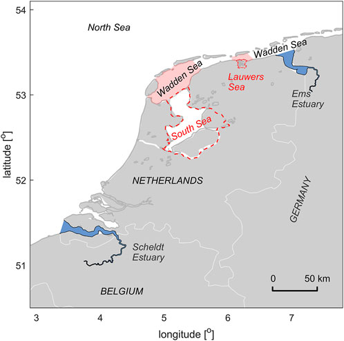
FIGURE 1. Overview of the intervened coastal systems studied in this paper: the two tidal basin closures in the Wadden Sea (Lauwers and South Sea, both indicated with red dashed lines), the Ems Estuary and the Western Scheldt (in blue). The South Sea was connected with the Western Wadden Sea (shaded red); the Lauwers Sea with the Zoutkamperlaag basin (shaded red as well). Both the Ems and Scheldt estuary are drawn exactly up to the tidal limit.

FIGURE 2

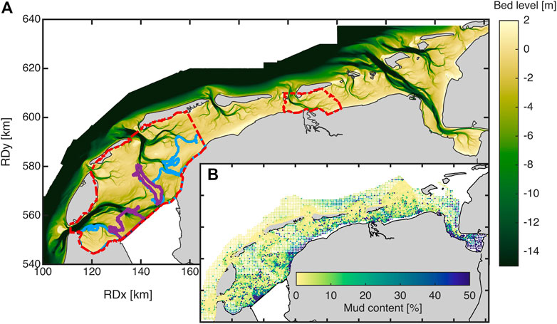
FIGURE 2. Wadden Sea bathymetry (A), in meter below local reference level NAP) and mud content (B), using the Dutch National Coordinate System (RD). The red dashed lines define the tidal basins of the Western Wadden Sea (left) and the tidal basin connecting to the Lauwers Sea (Zoutkamperlaag; right). The purple polygons within the Western Wadden Sea demarcate rapidly accreting channels; the blue polygons rapidly accreting shoal complexes (see Colina Alonso, 2021). The bathymetry is publicly available from the Ministry of Public Works; the mud content is computed from the Sedimentatlas (Rijkswaterstaat, 1998).

The largest closure was that of the 3,600 km² large South Sea basin, leading to migration and infilling of tidal channels and sedimentation on flats. The response of the Western Wadden Sea can be analyzed using a set of nine composite bathymetric maps constructed from observations dating back to 1933 (see Colina Alonso et al., 2021) for details). The sediment distribution has been mapped in detail in 1990, and is annually surveyed since 2015 (Colina Alonso et al., 2021). This availability of data combined with the observation that the distribution of sand and mud did not vary greatly over time (Colina Alonso et al., 2021) allows differentiation between net deposition of sand and mud. In Section 3.2 we will revisit their data and analyze the response timescales of the Western Wadden Sea to closure of the South Sea, differentiating between muddy and sandy deposits. We will hereby investigate the response of the basin as a whole, but also a number of smaller strongly depositional subareas identified by Colina Alonso et al. (2021) (see also Figure 2) dominated by tidal flats or tidal channels. Tidal channels are herein defined as the area below mean low water; tidal flats are defined as areas between mean low and mean high water.

The closure of the much smaller Lauwers Sea (90 km²) had a more localized impact compared to that of the South Sea. Yet, it did result in a net eastward shift of the tidal divides of its tidal basin (the Zoutkamperlaag), and net accumulation of sediment (Oost, 1995; Wang et al., 2013). This eastward shift resulted in a temporal change in the surface grain size distribution. Huismans et al. (2023) differentiate between sedimentation in channels and on shoals and between sand and mud. They calculate the historic sand and mud infilling volumes using high-resolution bathymetry and sediment composition data (Sedimentatlas; Rijkswaterstaat, 1998 and SIBES; Bijleveld et al., 2012) in combination with deep sediment cores (van Ledden et al., 2006) located in the tidal channel (where accretion rates where the largest). They show that accretion rates are much larger in the channels then over the shoals, and that infilling rates of mud were especially high in the vicinity of the closure. In Section 3.2 we revisit their results, analyzing the response timescales of sand and mud to the closure.

2.2 The Ems Estuary: Tidal amplification and hyperturbidity in response to deepening

The Ems estuary, situated on the Dutch-German border (Figure 1), is approximately 100 km long from its mouth (at the island of Borkum in the Wadden Sea; km 103 in Figure 3A) to the tidal limit (the weir at Herbrum; km 0). The outer estuary is typically 5–10 km wide and predominantly sandy but becomes progressively muddy in the landward direction, narrowing to a 70 m wide channel at its tidal limit (the weir at Herbrum). The Ems has a total catchment area of 17,934 km² (Krebs and Weilbeer, 2008) and an annual average discharge of 79 m³/s, varying between 45 m³/s (summer average) to 114 m³/s (winter average) (NLWKN, 2018). The estuary has undergone large anthropogenic changes in the past decades to centuries. Land reclamations carried out in the past 500 years have greatly reduced the intertidal area of the outer estuary (van Maren et al., 2016). Human interferences have accelerated in the past 50 years, with the construction/extension of three ports requiring an approach channel depth up to 12 m (van Maren et al., 2015a). The tidal channels in the Ems Estuary were historically organized as distinct ebb- and flood channels (van Veen, 1950). Some of these channels have degenerated as a result of channel deepening and land reclamations, effectively transforming parts of the estuary into a single-channel system.

FIGURE 3

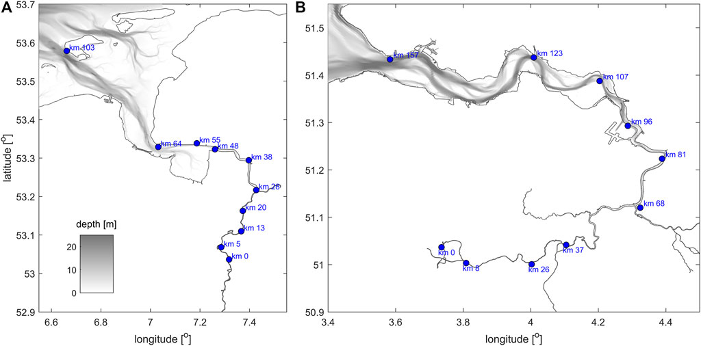
FIGURE 3. Gauging stations in the Ems Estuary (A) and Scheldt Estuary (B), with bathymetry in meter below local reference datum (NAP). The Ems Estuary has been deepened between km 0 and its mouth at km 103. The Scheldt estuary has been deepened between km 81 and 157, and sand mining took place between km 68 and 157.

The lower Ems River is deepened from approximately 4 m to almost 8 m (below MHW) to provide access to a shipyard (in Papenburg) located close to the tidal weir (in Herbrum), resulting in a transition to hyperturbid conditions; the present-day lower Ems River is characterized by thick and mobile fluid mud with concentrations up to 200 kg/m³ (Papenmeier et al., 2013). The present-day hyperturbid conditions are believed to result from deepening that took place in the early 1990s. Deepening led to tidal distortion, initiating a positive feedback mechanism where progressively more sediment was imported, which lowered the apparent hydraulic roughness and further increased tidal amplitudes (Winterwerp et al., 2013; de Jonge et al., 2014; van Maren et al., 2015b; Dijkstra et al., 2019a; Dijkstra et al., 2019b). However, the tides in the lower Ems river have been almost continuously amplifying since the 1950s (Figure 4A), and are therefore not only responding to the 1990s deepening. Even more, tidal amplification only appears to be weakly correlated to capital dredging works–even the major deepening that took place between 1991 and 1994 (from 5.7 m to 7.3 m) seems to have a moderate impact on the tidal range. In Section 3 we will analyze the impact of capital dredging works on tidal amplification in more detail using exponential decay functions.

FIGURE 4

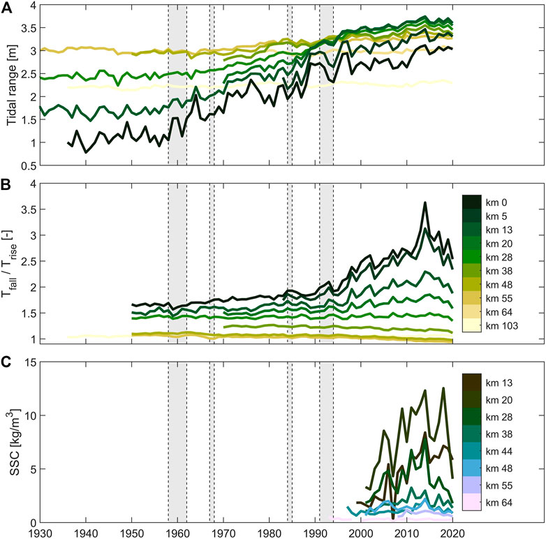
FIGURE 4. Annual tidal range (A), ratio of the duration falling tide to rising tide (B) and annually averaged SSC (C) measured at gauging stations in the Ems Estuary and lower Ems River. The grey shades indicate phased of deepening. Between 1958 and 1962 the approach channel to Emden was deepened and the training wall separating it from the Dollard upgraded; the channel between Leerort and Papenburg was deepened to 5 m (below MHW) and the section between Papenburg and Herbrum narrowed. In 1967 the channel up to Leerort was deepened up to 5.5. The entire channel (Emden–Papenburg) was gradually deepened to 5.7 m (1984), 6.3 m (1991) and 7.3 m (1994). The station names are expressed as their distance from the tidal limit (the weir at Herbrum) and correspond to the following gauging station names: Herbrum (0 km), Rhede (5 km), Papenburg (13 km), Weener (20 km), Leerort (28 km), Terborg (38 km), Gandersum (44 km), Pogum (48 km), Emden (55 km), Knock (64 km) and Borkum (103 km; the estuary mouth). SSC and water level locations sometimes differ and are therefore plotted in different colors, but for both the light tones are seaward stations and dark tones landward stations. All data is provided by NLWKN.

In contrast, tidal duration asymmetry (here expressed as the ratio of the duration of the falling tide over the duration of the rising tide $T_{f a l l} / T_{r i s e}$ ) responds much more clearly to the 1991–1994 deepening than the tidal range. At the upstream weir at Herbrum, the duration of falling tide increases from about two times the rising tide period to three times the rising tide period (Figure 4B). This change is associated with an increasing flood dominant sediment transport. More seaward located stations display a lower asymmetry magnitude (less flood-dominant) but a similar relative change resulting from deepening. The SSC rises sharply in response to deepening (Figure 4C) because of a positive feedback mechanism between tidal amplification, sediment import and apparent hydraulic roughness described above. Continues monitoring (as in Figure 4C) only started when the estuary was already turbid, but extrapolation of the data supports that the turbidity increased in the early 1990s. Interestingly, this increase in turbidity is not associated with obvious changes in the tidal amplitude (because these were already gradually increasing for a prolonged period of time) but with a change in tidal duration asymmetry.

A final striking observation is that the tidal amplitudes, asymmetry and SSC no longer increase (or even slightly decrease) after 2015. It seems that the estuary has achieved a new quasi-equilibrium around this period (in which SSC and the tidal range are in equilibrium with maintenance dredging strategies). Apparently, the deepening in the early 1990s required an adaptation period of ∼20 years, realized by an increase in tidal duration asymmetry and resulting increase in SSC.

2.3 The Scheldt estuary: Tidal amplification in response to land reclamations and deepening

The Scheldt estuary (Figure 1) stretches over a distance of 160 km from its mouth at Vlissingen (km 157 in Figure 3B) to the limit of tidal influence at the weir in Ghent (km 0). The Scheldt River has a catchment area of about 22,000 km² and an average freshwater discharge of about 100 m³/s, with minimum and maximum values between 20 and 600 m³/s (Fettweis et al., 1998). The estuary is composed of three distinct parts; the Western Scheldt (the multi-channel system up to 10 km wide) the lower Sea Scheldt (between the Dutch–Belgian border and the freshwater limit upstream of the Port of Antwerp where the estuary is 400 m wide), and the upper Sea Scheldt (up to the tidal barrier at Ghent with a width of ∼50 m). Most engineering works (rectifications of the river and embanking intertidal areas) in the upper Sea Scheldt took place between 1878 and 1904 (van Braeckel et al., 2006); land reclamation continued throughout the estuary until 1970.

Dredging-related impacts include capital dredging (channel deepening), maintenance dredging, and sand mining. The access channel was deepened during three capital dredging events: 1970–1976, 1997–1998 and 2008–2010. Dredged sediment (both during capital and maintenance dredging) was largely extracted from the lower Sea Scheldt until 1973 (65 million m³/y between 1950 and 1973; of which 23 million m³ as part of channel deepening from 1969 to 1973 (IMDC, 2013a). Dredging continued at similar rates after 1973 (∼2.5 million m³/y) but sediment was largely disposed within the lower Sea Scheldt. Sediment was still removed from the system through sand mining, averaging ∼1 million m³/y in the lower Sea Scheldt (between 1990 and 2009; IMDC 2013b) and ∼0.2 million m³/y in the upper sea Scheldt (2001–2010; Vandenbruwaene et al., 2017). Sand mining volumes prior to 1990 (lower Sea Scheldt) and 2001 (upper Sea Scheldt) are not known.

The various human interventions led to an increase in tidal amplitudes within the 120-year period, with tidal amplitudes increasing more strongly in the landward direction (Figure 5A). The most prominent increase took place during the deepening of 1971–1976. The tidal range in the lower Sea Scheldt (km 68–107) amplifies rapidly shortly after the 1971 deepening (Figure 5A) largely due to a lowering of the mean low water level (Vandenbruwaene et al., 2019a). The adaption period to this deepening appears to be ∼10 years between km 68–107 while the more upstream stations respond more gradually. The 1971 deepening not only influenced the tidal range, but also the tidal duration asymmetry (Figure 5B; see also Vandenbruwaene et al., 2019a; Vandenbruwaene et al., 2020). Since 1971 the tidal duration asymmetry in the lower and upper Sea Scheldt is decreasing (Figure 5B), i.e., the tide is becoming less flood-dominant, opposite to the trend observed in the Ems Estuary (Figure 4B).

FIGURE 5

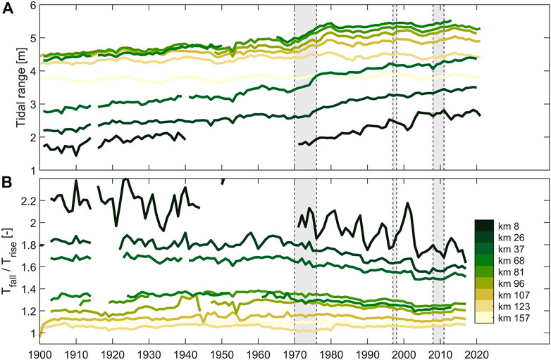
FIGURE 5. Annual tidal range (A) and ratio of the duration falling tide to rising tide (B) in the Scheldt estuary. The tidal range up to 2011 is from Winterwerp et al. (2013) and after 2011 from https://www.scheldemonitor.be/; ebb to flood ratios are from Vandenbruwaene et al. (2019a). The data is originally collected by the Dutch Ministry of Public Works and the Hydrological Information Centre (HIC) of Flanders Hydraulics Research. Periods of major deepening are indicated with grey shading. During the 1971–1976 deepening the river bed of the lower Sea Scheldt was lowered 1.5–2 m (van Braeckel et al., 2006). During the 1997–1998 deepening the access channels through the Western Scheldt was deepened with ∼1 m; the lower Sea Scheldt was especially deepened with ∼2 m between km 81 and 96 (IMDC, 2013a). The access channel was deepened with another 1.7 m seaward of approximately km 96 between 2008 and 2010 (IMDC, 2013b). Stations names (in km) are expressed as their distance from the tidal limit (the sluices at Gent) and correspond to the following gauging station names: Melle (8 km), Schoonaarde (26 km), Dendermonde (37 km), Schelle (68 km), Antwerpen (81 km), Liefkenshoek (96 km), Bath (107 km), Hansweert (123 km), and Vlissingen (157 km; the estuary mouth).

In order to better understand the effect of deepening on both tidal range and asymmetry, we compute changes in tidal range and changes in tidal duration asymmetry over three sections (Figures 6A–C) and compare these to morphological changes (the relative reduction of the intertidal area and the relative increase in channel depth) within these same three sections (Figures 6D–F). Section 1 is the upper Sea Scheldt between km 37 and 68 and was limitedly modified since the 1970s and where dredging volumes are small. Section 2 is the lower Sea Scheldt between km 68 and 96, a part of the estuary which includes the deepened and strongly modified Port of Antwerp. Section 3 (between km 96 and 123) is the transitional zone from the single-channel Sea Scheldt to the multi-channel Western Scheldt. In all sections tidal attenuation decreased (Section 1) or amplification increased (Sections 2, 3). The tides in Section 2 (km 68–96, i.e., the area around the port of Antwerp) clearly amplified in time during the 1971–1976 deepening (Figure 5A) but not over the channel length (Figure 6B). The steep tidal range increase over time observed at stations at km 68, 81 and 96 (Figure 5A) is therefore the result of tidal amplification generated in the more seaward located Section 3 (km 96–123; where the tides amplified from +10% before deepening to +20% after deepening–see Figure 6C).

FIGURE 6

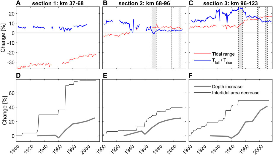
FIGURE 6. Change in tidal range and duration asymmetry (A–C) and in depth and intertidal area (D–F) for three sections in the Sea Scheldt. The change in tidal range (or ratio of falling tide to rising tide) is defined as the percentual increase of the tidal range (or ratio of falling tide to rising tide) in the landward direction per section. The change in depth is the average increase in the water depth per section below low water relative to the water depth in 1930. The change in intertidal area is the reduction of intertidal area by land reclamation (i.e., not resulting from morphological changes of these areas) relative to the intertidal area present in 1900 (i.e. a 70% change implies that 30% of the original intertidal area remains). The section between km 37–68 (Dendermonde–Schelle) is part of the upper Sea Scheldt where no deepening took place. The section between km 68–96 (Liefkenshoek–Schelle) is the lower Sea Scheldt including the port of Antwerp. The section between km 96–123 (Liefkenshoek–Hansweert) is the transition between the Western Scheldt estuary and the lower Sea Scheldt. The water depth and intertidal area data is from Vandenbruwaene et al. (2019b); see references in Figure 5 for origin of the tidal data. The grey shaded bars in panel (B) and (C) indicate periods of capital dredging.

There is a general tendency of the tidal duration asymmetry to increase until 1970 and decrease afterwards (Figure 5B), but these changes are largely generated in the seaward Section 3 (Figure 6C). The increase in asymmetry (up to 1970) is primarily the result of land reclamations (Figures 6D–F). In the period 1900–1970, 40%–80% of the intertidal area present in 1900 was reclaimed. Such loss of intertidal water storage typically leads to an increase in flood dominance (Friedrichs and Aubrey, 1988). Similarly, deeper channels promote ebb dominance (Friedrichs and Aubrey, 1988) and therefore the 1971–1976 deepening leads to a decreasing tidal duration asymmetry. And comparable to its effect on the tidal range, Section 3 controls the changes in duration asymmetry in the more landward sections as well (Vandenbruwaene et al., 2020): while the duration asymmetry strongly decreases shortly after deepening within Section 3 (Figure 6C), the change in tidal duration asymmetry within Sections 1, 2 is negligible (Figures 6A, B). The pronounced decrease in duration asymmetry over time throughout the upper and lower Sea Scheldt (Figure 5B) is therefore a response to interventions in Section 3 (and also seaward of km 123, because the asymmetry at km 123 decreases more strongly than at km 157–see Figure 5B).

No maintenance or capital dredging took place in the upper Sea Scheldt in the 1970s (IMDC, 2013a) and sand mining was very limited (Vandenbruwaene et al., 2017). Yet, the channel depth is increasing (Figure 6D) and the timescales involved in tidal amplification appear to increase in the landward direction (Figure 5A). The increase in tidal range observed here (Figure 6A) is therefore most likely a response to the increase in tidal amplitudes down-estuary (see also Winterwerp et al., 2013). Interventions down-estuary of Section 1 increase the tidal range in the upper reaches by up-estuary propagation of tidal waves with larger amplitudes. The resulting higher flow velocities remobilize sediments in the upper Sea Scheldt which are subsequently removed from the lower Sea Scheldt by dredging (either as maintenance dredging or by sand mining). The resulting local deepening of the upper Sea Scheldt (Figure 6A) then leads to a further increase in tidal amplitude (Figure 6B). This triggers a process in which the bed becomes progressively deeper and the tidal range larger.

The qualitative analysis of tidal changes over time and space suggests that the tidal amplitude in the lower Sea Scheldt around Antwerp (Section 2) mainly increased in the 1970s because of dredging (both capital and maintenance dredging and sand mining) of its downstream reaches (Section 3). These higher tidal amplitudes also propagate further landward (Section 1) where scouring of the river bed further amplified the tides; deepening is facilitated by removal of sediments from the lower Sea Scheldt through sand mining (to the present day) and dredging (until 1973). The period over which tidal amplification takes place therefore increases in the landward direction (from ∼10 years at km 68, the landward limit of deepening and most dredging efforts) to an almost continuous increase of tidal range at the tidal weir). In Section 3, we will analyze the impact of deepening in a more quantitative way using exponential decay functions (introduced hereafter). We will focus herein on dredging works between 1969 and 1973 because this event provided the largest sediment loss (∼23 million m³ in 4 years) but also led to tidal amplification (see Figure 5).

2.4 Computation of adaption timescales

Defining an adaptation timescale to an intervention also requires a reference condition that the system recovers to. This reference condition is morphodynamic equilibrium. It can be defined as the mutual adjustment of topography and fluid dynamics involving sediment transport (Wright and Thom, 1977). Morphodynamic equilibrium is timescale dependent: over geological timescales estuaries and tidal lagoons are temporary features drowning with sea level rise or filling in with fluvial sediment (Dalrymple et al., 1992). On the timescales of centuries, equilibrium may be defined as a condition with zero residual sediment transport for tide-dominated systems in absence of a sediment source (e.g., Lanzoni and Seminara, 2002). Zero residual transport cannot be attained for fluvial estuaries however, because of the permanent sediment source (Bolla Pittaluga et al., 2015) which led Zhou et al. (2017) to differentiate between static equilibrium (no changes), dynamic equilibrium without bed level changes, and dynamic equilibrium with bed level changes. But in reality the complexity of interacting processes is so large that estuaries seldom reach equilibrium (Perillo and Piccolo, 2011; Zhou et al., 2017). Following the definition of Bolla Pittaluga et al., 2015 the Ems and Scheldt estuaries cannot even be in equilibrium, because alluvial estuaries in morphological equilibrium cannot experience any amplification of the tidal wave propagating landward.

We therefore take a more pragmatic approach towards equilibrium. We define equilibrium as a condition were the changes in a parameter $X$ (which may be tidal range or bed level) are much smaller than the changes in $X$ in the years immediately following the intervention. The adaption $d X / d t$ of e.g. a sediment volume $X$ to a new equilibrium $X_{e}$ in response to a (relatively small) disturbance can then be formulated as [e.g., van Goor et al. (2003) and Kragtwijk et al. (2004)].

\frac{d X}{d t} = \frac{X_{e} - X}{τ} (1)

Herein $τ$ is adaptation timescale. Eq. 1 can be fitted to multiple data types (see the following section), providing values for $τ$ . The solution of Eq. 1 is an exponential function which is useful for a better understanding of $τ$ :

X (t) = X_{e} + (X_{0} - X_{e}) e^{- t / τ}

( 2)

Wherein X₀ = X (0). Eq. 2 shows that the morphological adaptation timescale $τ$ in Eq. 1 is the period the disturbance $X_{t} - X_{e}$ decreases to $1 / e \approx 0.368$ - see also Figure 7–i.e., the system has completed 63% of the total adaptation. At this point the system is still fully adapting to its disturbance, and therefore $τ$ does not adequately describe the timescale to an intervention. We therefore define a morphological halving time $T_{0.5}$ , which is the period the disturbance $X_{t} - X_{e}$ decreases to 0.5, as

X (t) = X_{e} + (X_{0} - X_{e}) 2^{- t / T_{0.5}} (3)

FIGURE 7

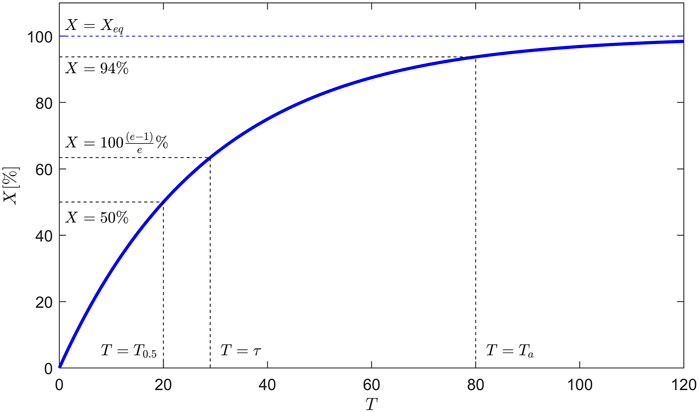
FIGURE 7. Definition sketch of timescales ( $T_{a}$ ; $τ$ ; $T_{0.5}$ ) and adaptation $X$ (in %, where the equilibrium is defined as $X_{e q}$ = 100%) for an exponential decay function. Half of the changes are achieved at $T = T_{0.5}$ , for this particular exponential decay function equal to 20 years. The adaptation timescale $T_{a}$ is then 80 years.

Which implies that $T_{0.5} = \ln (2) τ$ . The advantage of such a halving time is that it conveniently relates the timescale to the remaining quantity (i.e., 50% after 1, 25% after 2, and 12.5% after three halving times). We define our morphological adaptation time $T_{a}$ as the time required for $X$ to adapt to 93.75% (hereafter rounded to 94%) of the new equilibrium condition $X_{e}$ , which corresponds to $T_{a} = 4 \ln (2) τ$ (four halving periods). $T_{a}$ may be computed using Eqs 1, 2 (correcting $τ$ ) or directly using Eq. 3. The value of 94% is slightly arbitrary because an exponential decay function never reaches complete equilibrium. This introduces an uncertainty in the absolute value of the adaptation time which we will discuss in more detail in Section 4.1.

The morphological adaptation times are subsequently computed for two types of datasets (Table 1): bed level observations in the Dutch Wadden Sea and water level observations in the Ems and Scheldt estuaries. Bathymetric datasets that (1) cover the period from intervention to (near) equilibrium over the scale of a tidal systems and (2) are sufficiently accurate are very scarce. However, in many other systems, especially estuaries and tidal rivers, long and accurate water level observations are available. 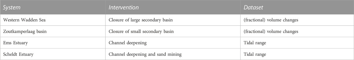For both the Wadden Sea closure examples and both estuary deepening examples we first manually define an initial disturbance (such as the 1932 closure of the South Sea or the 1970 deepening of the Scheldt estuary) and obtain values for $X_{e}$ and $T_{a}$ through a least-squares fitting procedure.

TABLE 1

TABLE 1. Dataset used for curve fitting per investigated system, including the type of intervention.

3 Results

3.1 Closure of the South Sea

The estimated response time $T_{a}$ of the Western Wadden Sea as a whole (Figure 8A) to closure of the South Sea is 64 years (i.e., the system attained a new equilibrium in the year 1996) according to an exponential decay fit with an R² of 0.98 (Table 2). Equilibrium is herein defined as $d V = 0.94 d V_{e}$ (see Section 3.1) which means that it may still be slightly adapting after reaching equilibrium (note that $T \to \infty$ for full equilibrium). Figure 8A also illustrates that the adaptation timescale of mud is much longer than that of sand. The sand volumes appear to have approached morphologic equilibrium after 50 years (i.e., in the 1980s) but the mud volumes are adapting much more slowly and is prognosed to attain equilibrium in 50 years from now. Even more, though the sand volume is the largest contributor (∼250,10⁶ m³) to overall volume change (∼350 10⁶ m³), the present-day mud accretion rates (∼1 10⁶ m³/year) exceed the current sand deposition rates. The western Wadden Sea as a whole does not appear to be importing sediments since ∼1990.

FIGURE 8

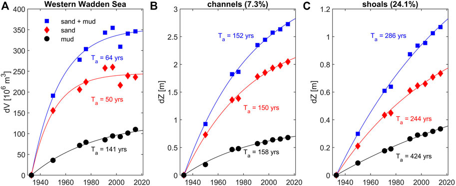
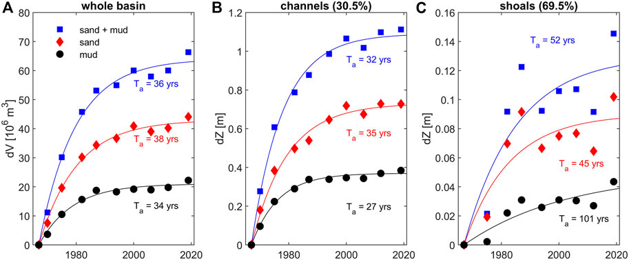
FIGURE 8. Total volume changes (A), in 10⁶ m³) of sand and mud in the Western Dutch Wadden Sea since 1933 (closure of the South Sea) from Colina Alonso et al. (2021) and accretion rates (in m) in rapidly infilling dead-end channels (B) and accreting fringing shoals (C). The size of the channel (shoal) area is 111,10⁶ m² (367,10⁶ m²) corresponding to a volume of 304,10⁶ m³ (392,10⁶ m³)–see Figure 2 for locations and Colina et al. (2021 for detailed historical changes). The adaption timescale Ta is computed using Eq. 1 (with colouring denoting the sediment type Ta is computed for). The channel and shoal percentage of panel (B) and (C) provide the spatial coverage relative to the total (A).

TABLE 2

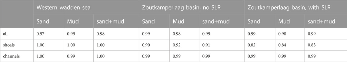
TABLE 2. R² values for the fitted functions in Figure 8 (Western Wadden Sea), Figure 9 (Zoutkamperlaag basin without SLR), and Figure 10 (Zoutkamperlaag basin with SLR).

However, sedimentation is not evenly distributed over the basin and therefore we additionally analyze rapidly infilling channels and shoal systems. Aggregating the volume changes of two infilling dead-end channels formerly feeding the South Sea, and of three nearby shoal complexes (see Figure 2 for locations; Colina Alonso et al. (2021) for details) reveals that the adaptation timescales may be much larger on a local scale. Note that these detailed fits achieve even higher levels of accuracy, with R² values between 0.99 and 1.00 (Table 2). The abandoned tidal channels (7.3% of the total area size) are estimated to reach a new dynamic equilibrium 150 years after closure, with remarkable little difference in sand and mud adaptation timescales (Figure 8B). The response time of the shoal complexes (24.1% of the total area) is in the order of centuries, with sand volumes attaining equilibrium after ∼250 years and the mud volumes after ∼400 years (Figure 8C). These adaptation timescales are the longest within the Western Wadden Sea, because the selected areas constitute strongly depositional areas. This also follows from the total amount of sediment depositing on the selected shoals and channels in Figures 8B, C. Their combined volume is 696,10⁶ m³ (i.e., double the net volume change in the Western Wadden Sea; 350,10⁶ m³) showing that some of the sediment depositing on the shoals and in the channels has been eroded elsewhere within the western Wadden Sea (see also Elias et al., 2012). Even more, with negligible sand deposition in the total Western Wadden Sea since 1990 (Figure 8A) while sand deposition over the selected flats (Figure 8B) and channels (Figure 8C) is structural implies that sand erosion is structural elsewhere in the Wadden Sea. Apparently the Western Wadden Sea adapted in two stages to closure of the South Sea: a first phase during which sediment was internally redistributed and sand and mud was imported from outside the Wadden Sea (i.e. the North Sea), and a second phase where sand and mud are still internally redistributed but only mud is imported from the North Sea.

3.2 Closure of the Lauwers Sea

The Lauwers Sea was much smaller than the South Sea (3,600 vs. 90 km²; a factor 40) resulting in much shorter adaptation timescales to the closure (Figure 9). The Zoutkamperlaag tidal basin adapted in ∼40 years, with the flats responding more slowly than the channels. The sedimentation rates over the shoals are quite low, and due to the relatively weak response to closure compared to background variation, the R₂ values are low (0.90–0.92) compared to the channels (0.99). Especially the response time of the mud fraction deposited on the flats is much longer (nearly 150 years). Interestingly, the net volume change of the tidal basin in response to closure of the Lauwers Sea is only ∼7 times smaller than the volume change resulting from closure of the South Sea (75 vs. 450,10⁶ m³) with the channels responding ∼5 times faster to closure of the Lauwers Sea and the shoals 9 times faster. This suggests a relation between the total net volume change and adaptation timescales.

FIGURE 9

FIGURE 9. Total volume changes (a, in 10⁶ m³) of sand and mud in the Zoutkamperlaag basin influenced by closure of the Lauwers Sea (see Figure 2 for location), and accretion rates (in m) in the tidal channels and on the shoals. The volume changes have been converted to accretion rates according to their areal size (46.0 10⁶ m² for the channels and 104.6 10⁶ m² for the shoals). The adaption timescale Ta is computed using Eq. 1 (with colouring denoting the sediment type Ta is computed for). The channel and shoal percentage of panel (B) and (C) provide the spatial coverage relative to the total (A).

An important difference between the deposition rates on the Lauwers flats and deposition rates on the Western Wadden Sea flats is that the latter are much larger than Sea Level Rise (SLR) while deposition rates over the Lauwers flats are only ∼0.2 m in a 50-year period and therefore approach rates of SLR (∼0.1 m, Vermeersen et al., 2018). Hence, the timescales in Figure 9 may be influenced by adaptation to SLR, and not only to closure of the Lauwers Sea. In order to separate the potential contribution of SLR to these timescales, we assume the Lauwers basin kept pace with SLR. Over the period 1930–2020 the mean sea level in the Wadden Sea increased 1.38 mm/y (based on the average of five long-term gauging stations operational in the Dutch Wadden Sea, see Figure 10) which is in line with earlier estimates by Vermeersen et al. (2018) but lower than average SLR in the German Wadden Sea (Benninghoff and Winter 2019). Subtracting potential SLR adaptation from observed accretion rates and volumes (see Figure 11) significantly reduces the computed adaptation timescales over the shoals (∼85 years decreasing to ∼52 years). Especially the adaptation time of the mud contribution decreases because mud constituted the weakest response to closure (only 8 cm) and is therefore easily influenced by the SLR signal. Adding an SLR component further weakens the strength of the signal relative to natural variation, resulting in a lowering of the correlation coefficient (Table 2).

FIGURE 10

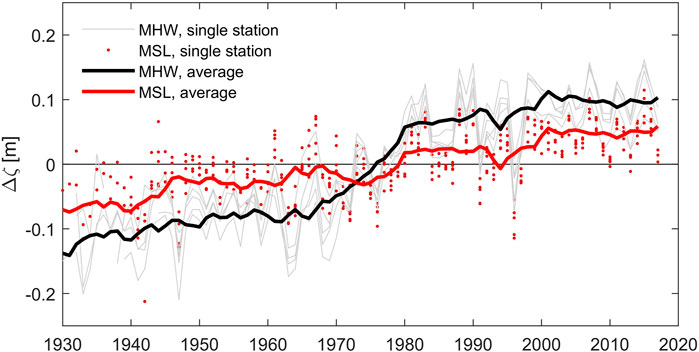
FIGURE 10. Mean sea level (MSL, in red) and mean high water (MHW, in black) anomalies in the Wadden Sea, based on the average of five long-term tidal gauges throughout the Dutch Wadden Sea (Den Helder, Harlingen, Kornwerderzand, Vlieland Port, West-Terschelling) starting observations around 1930 (data from the Dutch Ministry of Public Works). MHW is defined as the annual average of all high waters for a specific year; the MHW anomaly (per station) is defined as MHW minus the long-term average MHW (over the period 1930–2020). MSL is defined as the annual mean water level; the anomaly is computed similar to that of MHW. The average MHW and MSL anomalies are smoothed with a 3 years running mean for visualization purposes.

FIGURE 11

FIGURE 11. As Figure 9, but with volume changes corrected for SLR (using the curve from Figure 10).

The rate of SLR may even underestimate the autonomous development of the Lauwers basin. Even though the average SLR rate was 1.38 mm/y over the period 1930–2020, the rise in mean high waters levels (MHW) was 2.86 mm/y (based on data presented in Figure 10) due to amplification of the semi-diurnal tidal constituents (Colina Alonso et al., 2021). The greatest increase in MHW was recorded in the period 1960–1980 for reasons which so far remain unknown. If it is assumed that the shoals grow with MHW levels (rather than with MSL) than the adaptation timescales to closure of the Lauwers Sea may be even shorter. And although the exact role of SLR or MHW on sediment accretion is unknown (it is unclear to what extent the area actually grows with SLR) this analysis shows that adaptation timescales become more difficult to estimate when vertical accretion rates in response to closure become close to expected siltation rates due to SLR or MHW. On top of this, the error in measurements also becomes progressively more important with a reduction of the strength of the signal.

3.3 The Ems estuary

Tides in the most upstream stations (Papenburg and Herbrum, km 13 and 0) started to amplify in response to the interventions around 1960 (Figure 4A). More downstream, tidal amplification appears to start (km 48) or accelerate (km 28) in response to the 1967 deepening (Figure 12). Tidal amplification accelerates at all stations landward of km 28 around 1990–it is not clear to what extent this can be attributed to the 1985 or 1990s deepening; the 1990s deepening sharply increased tidal duration asymmetry (Figure 4B), especially in these landward stations, and is very likely also responsible for the high turbidity levels (Figure 4C). It is therefore not evident whether the 1967 deepening or the 1990s deepening had a larger impact on amplification, and therefore we fit Eq. 1 to the data using two starting times. The first start time is 1970 (instead of 1967 because of the much larger data availability after 1970); the second is 1990.

FIGURE 12

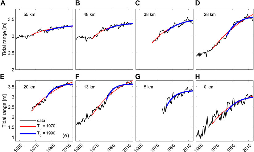
FIGURE 12. Observed (black) and fitted (blue and red) increase in tidal range A over time (panel (A–H), per station) along the lower Ems River. The red line is a fit of Eq. 1 against observations over the period 1970–2020 (except for station Rhede (km 5) where data is only available since 1986); the blue line over the period 1990–2020. The fitted values for T_a are given in Figure 13. The distance is measured relative to the tidal limit (the weir at Herbrum).

In the upper estuary (km 13–28), the tidal range increase between 1970 and 2020 cannot be described with an exponential decay function (1970 fit in Figure 12). This suggests that the system is not morphologically adapting to (only) the 1967 deepening. The tidal range increase from 1991 to 2020 does follow an exponential decay (1990 fit), suggesting that the upper estuary is primarily adapting to the 1991 deepening. Between km 28 and 55 the tidal range exponentially decays for both starting dates (1990 and 1970). This suggests that here the tides especially amplified in response to the 1967 deepening and that the impact of the 1990s deepening was weaker here than in the upstream reaches. This is supported by changes in tidal duration asymmetry: after 1990 the tides became especially asymmetric in the upper reaches (Figure 5B). 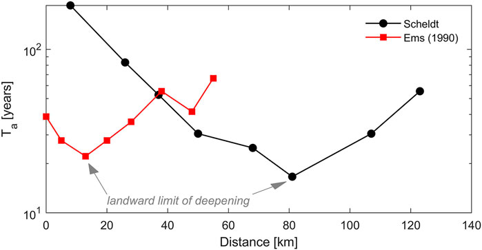The computed morphological response timescale $T_{a}$ of the section between km 38 and 55 is 40–50 years (since 1990)–see Figure 13) but since the changes here appear to be more strongly influenced by deepening in the 1970s the response time here should be closer to 60–70 years. Landward of km 38, the response time $T_{a}$ is 20–40 years (since 1990), indicating that these upper reaches are very close to reaching a new equilibrium. Strikingly, the morphological adaptation timescale is shortest at the landward limit of deepening (km 13) and increase logarithmically in both the landward and the seaward direction.

FIGURE 13

FIGURE 13. Adaptation timescales T_a to deepening as a function of distance from their upstream tidal limit (the weir at Herbrum for the Ems estuary and the sluices at Gent for the Scheldt estuary).

The R² values of decay functions to tidal range data is lower (Figure 14) than for the volumetric changes (Table 2). The R² coefficient is highest in the more upstream reaches of the estuary, because the seaward stations display a smaller rate of change. But the accuracy also decreases in the most upstream stations (<10 km from the tidal limit), possibly because of the progressive influence of river discharge. The R² values for the 1970 fit are higher than for the 1990 fit, which is surprising given the apparent better fit (Figure 12). The RMSE, however, is much lower for the 1990 fit than for the 1970 fit thereby better agreeing with visual observations.

FIGURE 14

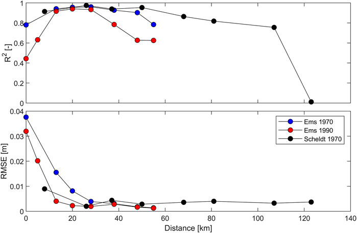
FIGURE 14. R² and RMSE for the function fit in the Scheldt Estuary and for the Ems Estuary starting in 1990 and 1970.

3.4 The Scheldt estuary

The observed changes of tidal amplitude in the Scheldt estuary follow an exponential decay in time since the 1970s deepening (Figure 15). Most striking is that a new equilibrium was attained fastest at km 81, while adaptation was slower in both the landward and seaward direction. The channel was deepened from km 81 (the port of Antwerp) in the seaward direction. The seaward increase in adaptation time may be related to the increase in channel width (the channel at km 123 is ∼10 times wider than the channel at km 81) and the associated increase in intertidal area, but also to the wider range of interventions (dredging activities including sand mining). Therefore we focus on changes in tidal dynamics in the landward direction (km 0–81). Visually, the time needed to adapt to the 1970 deepening appears to be around 10–20 years at km 81 km (only slightly exceeding the actual capital dredging period of 5 years). At the tidal limit however, the tidal river appears to be adapting to the deepening to this day. We will therefore investigate the adaptation timescales in more detail hereafter.

FIGURE 15

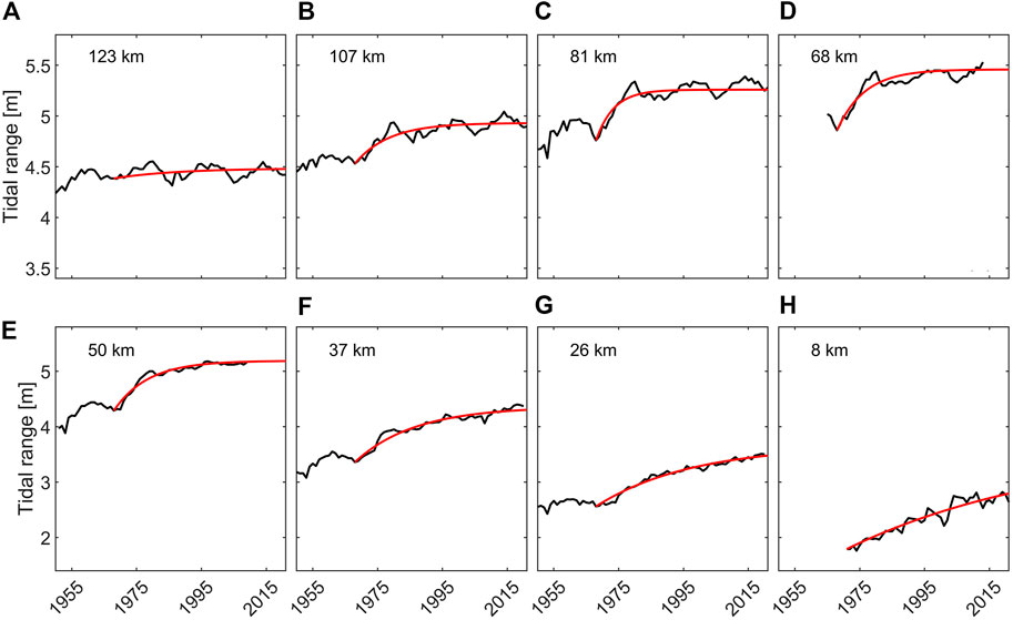
FIGURE 15. Observed (black) increase in tidal range A over time (panel (A–H), per station) for the Scheldt Estuary. The red line is a fit of Eq. 1 against observations over the period 1970–2020 (A–H) fitted values for T_a are given in Figure 13. The distance is measured relative to the tidal limit (the sluices at Gent). Note the different y-scaling for the upper and lower panels.

The adaptation timescale $T_{a}$ in the Scheldt estuary is 16 years at the port of Antwerp (km 81), gradually increasing in the landward direction to ∼200 years (Figure 13). This long response time may be the result of autonomous deepening of the upper Sea Scheldt (km 0–68) in the 1970s (Winterwerp et al., 2013). The reasons for this autonomous deepening have until now not been adequately explained, and our methodology provides important new insights into underlying mechanisms. Especially the observation that the adaptation timescale increases exponentially in the landward direction from the landward limit of dredging is strong evidence that autonomous deepening of the upper Sea Scheldt is (at least partly) resulting from deepening works in the lower Sea Scheldt and Western Scheldt. Apparently, deepening of the Western Scheldt and lower Sea Scheldt in the early 1970s led to tidal amplification in the upper Sea Scheldt. The larger tidal volume triggered erosion in the upper Sea Scheldt and the resulting deepening of the channel further increased the tidal range. This positive feedback mechanism led to autonomous deepening of the upper Sea Scheldt and an increase in its tidal range.

The R² values in the Scheldt estuary are slightly higher than this in the Ems estuary (Figure 14). The R² values decrease in the seaward direction (similar to the Ems estuary) but a difference is that the Scheldt tidal signal displays a much more pronounced 18.6-year nodal cycle (especially evident in Figure 15A). As a result, the R² values decrease between km 68–107 even though visually the decay function appears to describe the data well.

4 Discussion

4.1 Methodology

We have applied a simple exponential decay function to determine the response time of estuarine systems to an intervention. Before interpreting these results in more detail, we first revisit the accuracy of the exponential decay function fit. For this purpose, we will discuss 1) the assumptions underlying the approach, 2) the definition of equilibrium, 3) the effect of the start time of the fit, and 4) the accuracy of the fit.

Two mathematical assumptions underlying our approach, related to the rate of change and to coupling of sand and mud, will be shortly revisited here. Eq. (1) describes the adaptation speed $d X / d t$ of a quantity $X$ to a new equilibrium $X_{e}$ in response to a relatively small disturbance. For these conditions there is no fundamental change in processes driving changes in $d X / d t$ . The method therefore assumes that for instance in the Wadden Sea the mechanisms shaping the basin remain the same (i.e. largely transport by tidal currents) and not a relative change in e.g. wave-driven resuspension in response to bathymetric changes. We have, however, no indications that relevant transport mechanisms have changed in the Wadden Sea or both estuaries, nor do our data reveal any such change. A second assumption related to the methodology is the individual fitting of sand and mud volume changes. We independently fit the changes in sand volume, mud volume, and the total volume, and the sum of the mud and sand volume change may therefore differ from the total volume change. The difference between the summed and the total volume therefore provides an error estimate. For the Western Wadden Sea the equilibrium volume is 376,10⁶ m³ when fitting mud and sand independently, but 354,10⁶ m³ when fitting total volume changes, implying a 6% error. For the Lauwers application the total and the sum of volumes are the same (each 74,10⁶ m³). Although coupled fitting could improve the accuracy of the Western Wadden Sea estimates, we believe that the error is sufficiently small to allow independent fitting. A third assumption is related to the use of an exponential decay function to describe the various datasets, but these aspects will be elaborated in more detail in Sections 4.2, 4.3.

A second point influencing the accuracy of the method is the definition of equilibrium, for two reasons. We have now defined 94% of change as equilibrium. It is important to realize that there is no true mathematical equilibrium because an exponential decay function never reaches equilibrium. The definition of equilibrium therefore becomes arbitrarily. We have chosen a value of 94% because this approaches 2 standard deviations in a normally distributed dataset. This value corresponds intuitively to ‘equilibrium’ when evaluating the examples presented in this paper. At a two time larger adaptation time ( $T_{a} = 8 \ln (2) τ$ ) the sediment volumes or tidal range has completed 99.6% of its equilibrium change, which is excessively long. A second aspect of equilibrium is the concept of equilibrium itself. We do not define equilibrium as strict as e.g. Lanzoni and Seminara (2002) or Bolla Pittaluga et al. (2015) which would not allow equilibrium to exist in anthropogenic estuaries (or in dynamic systems in general–see Perillo and Piccolo (2011) or Zhou et al. (2017). Instead we adopt a more pragmatic approach where we define equilibrium as a condition were changes are much smaller than shortly after the intervention. While acknowledging this simplification in our methodology, we believe it has minor impact on our result given the large response to interventions in our examples.

A third point is related to the starting date of the fit, and data requirements around this date. The fact that the initial data is user-specified introduces a bias. A solution is to a add the starting date as an unknown variable to be solved as part of the least-squares fitting procedure. However, a user-defined value ensures constant starting dates throughout a system and allows accounting for availability of data as well (as done for the Ems 1970 fit). For stations in the Ems where water levels appeared to be primarily influenced by the 1970 deepening (km 38–km 55), the adaptation time of the 1990 fit was on average 16 years shorter than for the 1970 fit. Using a later point in time to initiate the exponential decay fit therefore does not introduce substantial errors (as long as the additional time is added after fitting). A related aspect that is especially relevant for bed levels is the temporal resolution of the data around the intervention. In the Scheldt estuary, bathymetric data is available 10 years before the 1970s deepening, during deepening, and 10 years after deepening. With adaptation timescales starting at 10 years (at the landward terminus of deepening) such a temporal resolution of data is insufficient to accurately resolve the exponential decay (and therefore determine adaptation timescales). This temporal resolution is less stringent for the Wadden Sea because the response timescales are much larger.

A fourth point of attention when discussing the accuracy of the method is the accuracy of the fit itself. The R² values of the volume fits are very high (typically between 0.97 and 1.00), suggesting a high level of accuracy. The reason that the correlation coefficient is so high is that sedimentation rates are high, and disturbances from measurement errors and/or other interventions are small. The correlation coefficient is lower for shoals experiencing smaller bed level changes (the Lauwers basin: ∼0.91 without accounting for SLR, ∼0.83 when accounting for SLR). The R² values of the exponential decay functions are lower for the tidal range data than for the volumetric changes. Typically the highest correlation coefficients are in the more upstream reaches of the estuaries (typically ∼0.95) where the response to deepening is large and variability introduced by the 18.6 years cycle is relatively small, while the effect of river discharge is also relatively weak.

Despite its simplicity and (as our results suggests) usefull application to describe tidal and bed level data, exponential decay functions are rarely, if ever, used to quantify adaptation timescales. Exponential functions have been fitted to bed level data in order to distinguish erosion minima and multiple erosion phases (Simon et al., 2016) but not, to the authors knowledge, to extract adaptation timescales. A change in tidal range has not been quantified using exponential decay functions (again to the authors knowledge), and therefore also never to extract adaptation timescales. In the next two sections, we will address the relevance of our findings in more detail focussing on adaptation timescales of tidal basins and estuaries.

4.2 Adaptation timescales of tidal basins: Bed level data

Tidal basins such as those in the Wadden Sea are affected by closure of tidal subbasins (such as the Lauwers and South Sea), SLR and, on a more local level, the maintenance of navigation channels. According to Wang et al. (2018) the large observed average accretion rates in some parts of the Wadden Sea are largely the result of closure of the Lauwers Sea and South Sea. This is illustrated by the rapid increase of tidal flat height (∼10 times the rate of SLR) in the Western Wadden Sea, showing that they are not predominantly growing with SLR but are mainly responding to other processes or interventions. Similarly large accretion rates of shoals were observed in the German Wadden Sea (with tidal flats accreting at ∼0.4–2.2 cm/y and channels eroding at 0.2 cm/y; Benninghoff and Winter 2019), the Weser estuary (tidal flats accreting 1.3–5.6 cm/y; Benninghoff and Winter 2018) and the Western Scheldt (tidal flats accreting on average at a rate of almost 1 cm/yr between 1955 and 2014; de Vet et al., 2017). In the Western Scheldt, the large accretion rates are attributed to channel deepening and disposal of dredged sediments whereas the mechanisms explaining the high deposition rates in the German Wadden Sea remain largely unexplained. The apparent common observation of high sedimentation rates over the tidal flats suggests a large-scale process (such as SLR or the observed rise in MHW) to be a controlling factor. But if the increase in MSL or MHW is controlling sedimentation, then sedimentation rates larger than the rise in MSL or MHW are unlikely (see e.g. Elmilady et al., 2020) which then suggests that closure of the South Sea is the controlling factor. Such control may be related to hydrodynamic changes or a loss of sediment sinks.

The various (secondary) tidal basins in the Wadden Sea (such as the South Sea and Lauwers Sea) were net sinks of sediment (van Maren et al., 2016). They developed in response to marine ingressions of peatlands which subsided due to anthropogenic cultivation (Vos and Knol, 2015). Because these basins were largely out of equilibrium, they provided efficient sediment sinks (exemplified by the several million m³ annually depositing in the Dollard Bay–see van Maren et al., 2016). The historical closure of tidal basins resulted in a sharp reduction of mud deposition on the intertidal and extensive supratidal flats covering large parts of the Northern coasts of the Netherlands and Germany (Vos and Knol, 2015) and hence to an increase in suspended fine sediments in the Wadden Sea (van Maren et al., 2016). For reference, the South Sea is 10 times larger than the Dollard Bay, which was filling in with three million ton per year (van Maren et al., 2016), suggesting the increase in available sediments was probably large. We therefore hypothesize that the closure of the South Sea led to an instantaneous redistribution of sediments with an adaptation time scale of ∼60 years, but that its long-term impact is an increase in fine sediment availability throughout large parts of the Wadden Sea.

This increase in sediment availability triggered larger sedimentation rates on the tidal flats of the Western Wadden Sea but, given its prevalent west-to-east transport direction (Sassi et al., 2015), possibly also influenced fine sediment deposition in the German Wadden Sea (where deposition over intertidal areas sharply increased, as described above). However, in the German Wadden Sea local closures (see Reise, 2005) such as the Meldorfer Bucht (48 km²; completed 1978), the Lower Elbe (150 km²; completed 1979), and the Nordstrander Bucht (33 km²; completed 1987) may have had a larger impact on sediment availability. But independent of the mechanism causing higher sedimentation rates, it did lead to a decrease in flood-dominant sediment transport (or an increase in eb-dominant sediment transport) in the German Wadden Sea which will in time lead to a reduction in these sediment deposition rates (Hagen et al., 2022).

4.3 Adaptation timescales of estuaries: Tidal data

The mechanisms responsible for the increase in tidal amplitude in both the Ems and the Scheldt estuaries have been intensively studied (Winterwerp and Wang, 2013; Winterwerp et al., 2013; van Maren et al., 2015b; Dijkstra et al., 2019a; Dijkstra et al., 2019b; Dijkstra et al., 2019c; Wang et al., 2019), but the timescales associated with tidal amplification in response to interventions have so far remained unexplored. We have developed a robust and systematic methodology to process tidal gauge data, providing response timescales of estuarine systems. A strong indication of the reliability of our method to compute adaptation timescales to the governing interventions from tidal observations is provided by its strong spatial coherence. Even though each observation was individually analyzed for its response timescales $T_{a}$ , the computed values for $T_{a}$ are strongly coherent in space, with six subsequent stations (in both the Ems and Scheldt estuary) following a nearly perfect logarithmic increase in response times. In the Scheldt estuary, the response times increase in the landward direction, starting at the landward terminus of the channel deepening (the port of Antwerp). In the Ems estuary the shortest adaptation is also observed at the landward terminus of the channel deepening and similar to the Scheldt, the adaptation times increase in both the landward and seaward direction of this point.

A condition for applying an exponential decay function to water level data is that the changes in water levels are controlled by processes which respond exponentially to disturbances. The morphodynamic response of a channel to deepening is well known to be exponential (de Vries, 1975; van Goor et al., 2003). Our analysis suggests that the tidal amplification (Figure 6A) and autonomous deepening (Figure 6D) of the upper Sea Scheldt Estuary is primarily a morphologic response to tidal amplification resulting from downstream deepening in the early 1970s (Section 3.2), allowing the use of an exponential fit for analyzing the water levels. The Ems Estuary reacted differently to deepening, however. Our analysis revealed that the tidal amplitudes in parts of the lower Ems River are responding to multiple phases of deepening (and not only the 1990s deepening), but that the upper ∼20 km of the lower Ems River is primarily responding to the 1990s deepening. The increase in tidal range after 1990 is probably controlled by changes in hydraulic roughness (Winterwerp et al., 2013; van Maren et al., 2015b; Dijkstra et al., 2019a; Dijkstra et al., 2019b). A question which then arises is why the Ems and Scheldt responded differently to deepening, which will be addressed hereafter.

The Ems estuary has become hyper turbid (see Figure 4C), largely in response to the 1990s deepening. Changes in SSC are much smaller in the Scheldt estuary compared to the Ems estuary, although SSC likely increased in 2008–2009 in the upper Sea Scheldt due to fairway widening and deepening, and dredging and dumping activities (Cox et al., 2019). The positive feedback mechanisms between deepening and tidal amplification through enhanced sediment import and reduced apparent hydraulic roughness identified by Winterwerp and Wang (2013); Winterwerp et al. (2013) for the Ems Estuary raised concerns on the potential of hyperturbid conditions developing in other estuaries as well, notably in the Scheldt Estuary. Based on idealized modelling; Dijkstra et al. (2019c) concluded that a regime shifts towards hyperturbid conditions is unlikely for the Scheldt estuary because sediment availability is erosion-rate limited rather than supply limited (as in the Ems Estuary), and because deepening led to a decrease in tidal duration asymmetry (rather than an increase in tidal duration asymmetry, as for the Ems Estuary). This latter difference had, however, up to now not been systematically investigated based on tidal data.

The difference in duration of falling and rising tides (Figure 4B; Figure 5B) clearly shows an increase in flood-dominance in the Ems estuary following the 1990s deepening, but a decrease in flood-dominance following the 1970s deepening in the Scheldt estuary. This different response to deepening may in turn be explained by the available intertidal area. The larger the intertidal area, the more deepening leads to a reduction in flood dominance (Winterwerp and Wang, 2021). And even though the intertidal area in the Scheldt estuary strongly declined over time (Figures 6D–F), the amount of intertidal area is still larger than that along the lower Ems River where the intertidal area is only several meters wide. Reduction of intertidal area leads to an increase in tidal duration asymmetry, which is observed in the Scheldt estuary before 1970 (Figure 6).

Another factor potentially explaining the difference in both systems is the role of the tidal weir at km 0 (for both systems). Reflection of the tidal wave against a weir may lead to resonance and therefore amplification of the tides (Talke and Jay, 2020), which probably strengthened tidal amplification in the Ems Estuary (Schuttelaars et al., 2012) especially in combination with reduced hydraulic drag (Winterwerp et al., 2013). The impact of the tidal weir in the Scheldt river has not yet been rigorously verified, but deepening (both autonomous as in the upper Sea Scheldt and through dredging further seaward) may introduce a shift of conditions closer to resonance (similar to what may have happened in the Ems Estuary).

5 Conclusion

We have developed and applied a methodology to estimate the response timescales of human interventions and how these timescales vary in space using available morphological and hydraulic data. Fitting an exponential decay function to data with sufficient temporal resolution yields an adaptation timescale (and equilibrium value) of the tidal range or sediment volume changes. As an exponential function, by definition, never reaches true equilibrium–we define equilibrium to represent the situation after 94% of the change (in volume or tidal range) resulting from the intervention. The benefit of this methodology is twofold. First, it provides timescales of response of a certain system to an intervention. Secondly, and possibly more importantly, the spatial coherence of timescales provides important insights into the physical functioning of the system.

Exponential decay functions fitted to morphological data influenced by closure of a large (3,600 km²) tidal basin (the South Sea) revealed that the impacted basin imported sediment for a period of ∼60 years after closure, superimposed on internal redistribution of sediments. After this period sediment is still internally redistributed but especially fine sediments are imported and accumulating in the impacted basin. This fine sediment deposition may be the result of the loss of sediment sinks in the closed tidal basin. The timescales associated with closures with a smaller impact (a 90 km² basin, the Lauwers Sea) are more difficult to determine because the lower accumulation rates become progressively more influenced by natural adaptation to rising mean sea levels or high waters and by measurement errors. The spatial coherence is illustrated by the along-channel variation in adaptation time to dredging. Fitting exponential decay functions to tidal data reveals how adaptation timescales resulting from deepening and sand mining increase in the upstream and downstream direction (with the upstream increase more important in the Scheldt estuary and the downstream increase in the Ems Estuary).

Data availability statement

Publicly available datasets were analyzed in this study. This data can be found here: The raw data may be retrieved from https://www.scheldemonitor.be/ (waterlevel data in Belgium), https://waterinfo.rws.nl/ (waterlevel data in the Netherlands) and https://waterinfo-extra.rws.nl/monitoring/morfologie/ (bathymetry data in the Netherlands).

Author contributions

DM, AC, PV, and ZW contributed to the study conception and design. Material preparation, data collection and analysis were performed by DM, AC, AE, and WV. The first draft of the manuscript was written by DM and all authors commented on previous versions of the manuscript. All authors read and approved the final manuscript.

Funding

This work was funded by the Programme of Strategic Scientific Alliances between China and the Netherlands and the Zijiang Scholar Program of East China Normal University.

Acknowledgments

We are grateful for the Dutch Ministry of Public Works, the Hydrological Information Centre of Flanders Hydraulics Research, and the Niedersächsische Landesbetrieb für Wasserwirtschaft, Küsten-und Naturschutz (NLWKN) for providing data. Frederik Roose is acknowledged for instructive comments on the manuscript. This manuscript improved considerably through the valuable suggestions of four reviewers.

Conflict of interest

The authors declare that the research was conducted in the absence of any commercial or financial relationships that could be construed as a potential conflict of interest.

Publisher’s note

All claims expressed in this article are solely those of the authors and do not necessarily represent those of their affiliated organizations, or those of the publisher, the editors and the reviewers. Any product that may be evaluated in this article, or claim that may be made by its manufacturer, is not guaranteed or endorsed by the publisher.

References

Benninghoff, M., and Winter, C. (2018). Decadal evolution of tidal flats and channels in the Outer Weser estuary, Germany. Ocean. Dyn. 68 (9), 1181–1190. doi:10.1007/s10236-018-1184-2