3D anisotropic full-waveform inversion for complex salt provinces

Seismic imaging and inversion become extremely challenging when dealing with salt structures. Conventional state-of-the-art full-waveform inversion (FWI) fails to recover those features in areas where salt is present. A widely used solution in industry, however, involves substantial human interpretation. In this study, a regularized isotropic full-waveform inversion that penalizes the velocity drops in depth is introduced to recover the top parts of salt bodies. Then, an automatic salt flooding is applied to reconstruct deeper parts of the salt. Finally, in order to improve the accuracy of the inverted model, which is strongly affected by anisotropy, an anisotropic FWI is used to update the velocity model. We tested the approach on both synthetic and field datasets. Our FWI results revealed satisfying salt recovery as well as detailed velocity features in areas close to salt bodies.

1 Introduction

A typical salt dome containing halite and anhydrite rocks is mostly impermeable. As it moves upwards, it bends the strata of existing rocks, which forms pockets where petroleum and natural gas are usually trapped. As a result, the delineation of salt and subsalt is of high interest in oil and gas production. Tomography is a standard practice for salt delineation where the best possible sediment velocity model is first built. Then, a top-of-salt interpretation using sediment flood migration followed by a base-of-salt interpretation using salt flood migration is carried out. For complex areas with complex salt geometry, a number of salt scenario tests are also necessary, which is not only labor-intensive and time-consuming but also prone to human misinterpretation. Alternative approaches, based on artificial intelligence (AI), are proposed to build a salt velocity model (Araya-Polo et al., 2018; Rusmanugroho et al., 2022).

Seismic inversion plays a key role in delineating subsurface structures (Tarantola, 1984; Pratt et al., 1998; Shin and Min, 2006; Pan et al., 2016). The full-waveform inversion (FWI) technique, which is considered the most promising data-driven tool to iteratively build velocity models, was first proposed by Lailly (1984), which aims to build high-quality and resolution velocity models with high precision for seismic imaging. However, the presence of complex salts causing high velocity contrast fails to provide high-resolution velocity model building from seismic data. This is caused by various factors such as strong multiples and insufficient subsurface illumination caused by velocity complexities in the overburden. Brenders and Pratt (2007) demonstrated that it is possible to use FWI to build a salt velocity model from a smooth initial model. However, the frequency they used was as low as 0.5 Hz, which is much lower than the real case in field data. Since then, traditional processing procedures involve calculating various salt attributes (Jing et al., 2007; Berthelot et al., 2013; Wang et al., 2015) to detect salt boundaries. These attempts often require both geophysical processing skills and geological interpretation (Farmer et al., 1996; Jones, 2012; McCann et al., 2012). Shen et al. (2017) and Michell et al. (2017) applied FWI to successfully correct some salt structure misinterpretation based on the availability of low frequency and full azimuth of ocean-bottom node (OBN) data, which greatly improved subsalt delineation in the Gulf of Mexico (GOM). Zhang et al. (2018) proposed a time-lag FWI (TLFWI) which uses a time-lag cost function (Luo and Schuster, 1991; Chavent et al., 1994) to reduce amplitude errors in the standard data-mismatch cost function (Tarantola, 1984). Wang et al. (2019) further applied TLFWI to velocity model building for areas with the presence of salt bodies.

The edge-preserving technique such as total variation (TV), first proposed by Rudin et al. (1992) and introduced in image restoration by Vogel and Oman (1998), was used in the estimation of density contrast distribution from gravity data inversion (Farquharson, 2008; Martins et al., 2011). Compared to other sediments, salt bodies are steeply dipping complex-shaped structures with higher velocity and lower density. Based on this, Anagaw and Sacchi (2012) proposed the application of TV to acoustic velocity perturbation estimation. These edge-preserving techniques usually are very successful in salt top recovery. However, they would fail to recover the bottom of the salt body and the subsalt due to erroneous velocity estimations in the vicinity of the salt body. Therefore, some additional techniques are required to recover the rest of the salt body (especially the deeper part of the salt). Esser et al. (2016) proposed the automatic salt flooding into salt delineating, by which the position of bottom salt can thus be picked up precisely. Kalita et al. (2019) further applied TV to recover the sharp boundaries of salts. Additionally, he also implemented salt flooding to recover the bottom of salt bodies.

In this paper, we further implement this technique into anisotropic media by proposing a new gradient calculation equation and applying it into the misfit function with TV regularization and flooding terms. This study solves two cascading minimization problems to determine the velocity field from the salt-affected dataset, where an edge-preserving technique is first applied to invert the top part of the salt (using the regularized FWI). Then, the output of the edge-preserving technique is used as an input to recover the rest of the salt (using the automatic salt flooding). Finally, we test this approach on both synthetic and real datasets. Our FWI results have revealed satisfying salt recovery as well as detailed velocity features in areas close to salt bodies.

2 Theory

2.1 Isotropic FWI + TV

The minimization of the misfit function with regularization can be expressed as

$J_d\left(m\right)={\mathit{min}}_m{‖d_0-d_m‖}_2^2+{\lambda }_{TV}{‖m‖}_{TV}.(1)$

where m is the discretized Earth subsurface parameters defined at all space points, J_d (m) is the objective function, d₀ is the observed seismic data, d_m is the modeled seismic data, and $\lambda$_TV is the regularization parameter. In the aforementioned equation, $\lambda$_TV is a positive regularization parameter that controls the trade-off between the data misfit term and the amount of interface-preservation in the inversion process. When we use low-frequency data for isotropic FWI, the sharp edges and discontinuities, such as the top of the salt structures, are preserved. Furthermore, ||m||_TV can be denoted as

${‖m‖}_{TV}=\left|\nabla m\right|=\sqrt{m_x^2+m_y^2+m_z^2}.(2)$

2.2 Cycle skipping

However, if low-frequency data are missing or low-wavenumber components of the initial velocity model are inaccurate, the adjoint source will suffer from cycle-skipping issue, which occurs when the observed and predicted data mismatch by more than half a cycle (Leeuwen & Herrmann, 2013; Wu et al., 2014; Brossier and Singh, 2015; Pan et al., 2018). As a result, it leads the inversion to be trapped in a local rather than the global minimum. The adjoint source is shown in Figure 1; for example, when the arrival time is less than 40 ms, there is barely cycle skipping. With the increase in arrival time, cycle skipping can be detected and the adjoint source is severely affected.

FIGURE 1

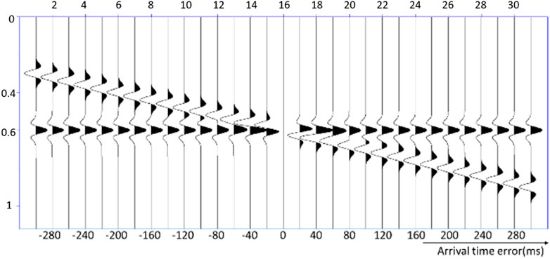
FIGURE 1. Adjoint source. Cycle-skipping issue can be detected when the arrival time is larger than 40 ms.

Cycle-skipped local minima are a major challenge for robust FWI. Theoretically, low frequencies are crucial for FWI to avoid cycle skipping because at low frequencies, both observed and modeled data should match within the half wave-cycle. To overcome cycle skipping, multiscale approaches are designed to update the model using the frequency bands from low to high (Chapman and Pratt, 1992; Alkhalifah, 2014).

Additionally, some other approaches, including modifying objective function, are also widely used to mitigate cycle skipping, such as cross-correlation, deconvolution, and Wiener filter. In this paper, the automatic cycle-skipping detection approach is applied, and then cycle-skipped energy is removed by modifying the adjoint source with a low pass filter. The adjoint source and the corresponding frequency distribution at different arrivals are shown in Figure 2. The classic Ricker wavelet is used as a reference source, and its frequency distribution is shown in Figure 2 a.1 and a.2. When the arrival time difference between the observed and modeled data is 20 ms (Figure 2 b.1–b.2) and 40 ms (Figure 2 c.1–c.2), respectively, there is no cycle-skipping frequency detected. Cycle skipping can be detected when the arrival time difference reaches 60 ms (Figure 2 d.1–d.2), where a notch appears at 16 Hz. Therefore, we design a notch detection algorithm, using which frequency components exceeding the notch point (notch frequency) can be filtered out. The highest frequency without cycle skipping can thus be estimated. The adjoint source of the L2 norm waveform difference FWI $v$ becomes

$\left.v={f\ast (d}_0-d_m\right),(3)$

FIGURE 2

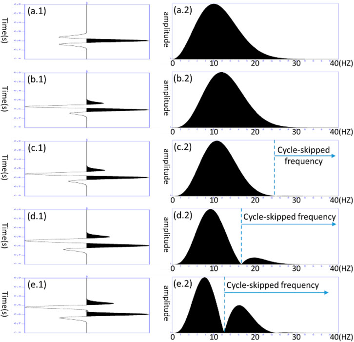
FIGURE 2. Detailed adjoint source and the corresponding frequency distribution at different arrival times. (a.1–a.2) Ricker wavelet as a reference source and its frequency distribution. (b.1–e.2) Adjoint source and the corresponding frequency distribution when the arrival time changes from 20 ms to 80 ms.

where f is a zero-phase low pass filter. It is similar to applying a low pass filter on the gradient to remove the high wavenumber local minimum. With a smoothed starting velocity model, the simulated shot gather of the first few iterations usually only contains diving waves, and the notch frequency can be easily detected from the residual between the synthetic and observed data. When reflections are involved, the automatic detection of the notch frequency becomes more complex due to conflicting events.

2.3 Automated flooding

A misfit function with Automated flooding can be expressed as

${\mathit{J}}_{\mathit{F}}\left(\mathit{q}\right)=\underset{\mathit{q}}{\mathbf{min}}\left\{{‖\mathit{q}-\mathit{u}‖}_{\mathbf{2}}^{\mathbf{2}}+{\mathit{\lambda }}_{\mathit{F}}{‖\mathit{q}‖}_{\mathit{F}}\right\},(\mathrm{4a})$

where J_F (q) is the objective function, q is the updated model, u is the model from regularized FWI (FWI + TV), and $\lambda$_F is the regularization parameter. In the aforementioned equation, it starts from the final output of isotropic ‘FWI + TV′ and penalizes the velocity drop in the model. Since the Automated flooding is thus applied everywhere, the high velocity is smeared across any region with a drop in the velocity field rather than only the salt body region. Therefore, in areas with low velocity, Automated flooding might have a detrimental effect. In that case, a minimal human intervention is required to flood from the top of the salt.

2.4 Anisotropic TTI FWI

Based on TV regularization and automated flooding in conjunction with isotropic FWI using low-frequency data, the geological shape of the salt body is anticipated to be well recovered. To obtain more detailed layered structures, an anisotropic TTI FWI is then applied. Although the FWI procedure is, in essence, an optimization problem to find the minimum of the objective function, a precise approximation of the anisotropic wave equation with less interactive noise from different wave modes is still considered the core of the objective function, which generates the modeled data that are used to calculate the data difference between observed data and will be ultimately contributed to the objective function. The approximated anisotropic q-P wave equation (Li et al., 2022) we used in this study is

$\frac{{\partial }^{2}p}{\partial t^2}=\left[v_h^2\left(k_{\stackrel{\sim }{x}}^2+k_{\stackrel{\sim }{y}}^2\right)+{v_{p0}^{2}k}_{\stackrel{\sim }{z}}^2\right]p-\frac{v_h^2-v_n^2}{1+\epsilon }\left[\frac{k_{\stackrel{\sim }{x}}^2+k_{\stackrel{\sim }{y}}^2}{k_{\stackrel{\sim }{x}}^2+k_{\stackrel{\sim }{y}}^2+k_{\stackrel{\sim }{z}}^2}\right]k_{\stackrel{\sim }{z}}^{2}p,(\mathrm{4b})$

where $k_{\stackrel{\sim }{x}}$, $k_{\stackrel{\sim }{y}}$, and $k_{\stackrel{\sim }{z}}$ are new wavenumbers in a rotated coordinate system and the lower case p used in this equation denotes the scalar wavefield of the P wave component. v_h and v_p0 are P wave velocity in horizontal and vertical direction, respectively; v_n is the normal move-out velocity; k_x, k_y, and k_z are wavenumbers in the original coordinate system without rotation; and $\epsilon$ is the Thomsen parameter.

The gradient of vertical P wave velocity, $g_{v_{p0}}$, can be expressed as

$g_{v_{p0}}=-2v_{p0}\frac{{\partial }^{2}p}{\partial z^2}-2v_{p0}\left(1+2v_h\right)\left(\frac{{\partial }^{2}p}{\partial x^2}+\frac{{\partial }^{2}p}{\partial y^2}\right)-4v_{p0}\left(v_n-2v_h\right)\frac{\partial }{\partial z^2}\left(\frac{{\partial }^{2}p}{\partial x^2}+\frac{{\partial }^{2}p}{\partial y^2}\right).(5)$

A real example is an OBN dataset from a Malaysian field that suffers from anisotropy, and a gas cloud imaging problem is used to validate our TTI FWI. Shallow gas layers are stacked on top of each other, which makes the travel path of the wavefield more complicated. A wipe-out zone can be seen under the gas layers, as shown in Figure 3A. The lowest frequency in these data is 7 Hz (below which the data suffered from low signal-to-noise ratio), as shown in Figure 3B. The 3D TTI FWI starts from 7 Hz to 12 Hz with a total of 45 iterations.

FIGURE 3

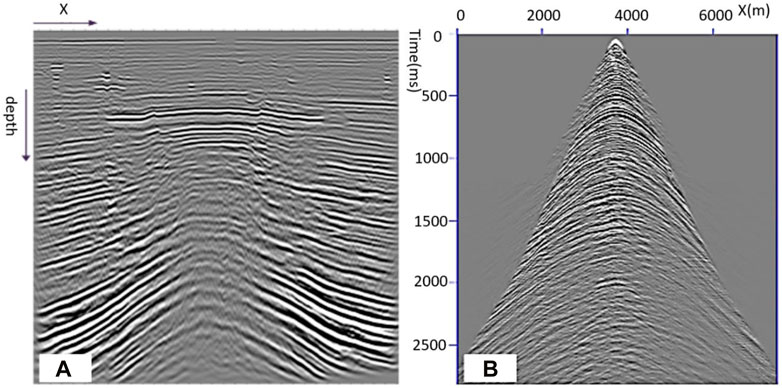
FIGURE 3. 2D OBN dataset from a Malaysian field. (A) PSDM stack shows a wipe-out zone under the gas layers. (B) Input shot gather for FWI after de-ghost, de-signature, and de-multiple.

Figure 4A shows the initial velocity model obtained by smoothing the tomography velocity model. The updated velocity model after running 45 iterations of TTI FWI is shown in Figure 4B. Compared with the initial velocity model, the updated velocity below the gas zone reveals more detailed geological layers, which matches the acoustic well logging data. In deeper parts, even more layered structures can be detected, where a fault-like structure is distinctively present, as shown in Figure 4B.

FIGURE 4

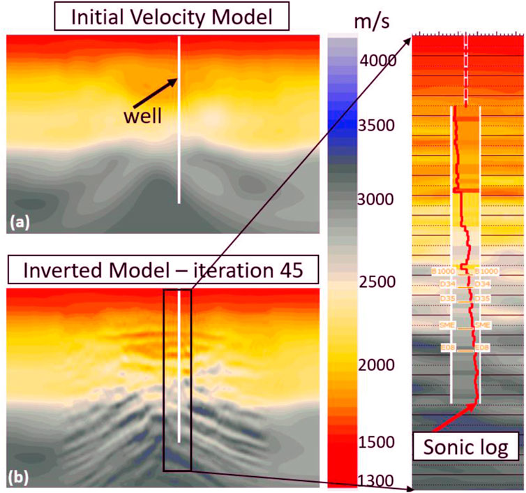
FIGURE 4. (A) Initial velocity model obtained by smoothing the tomography velocity model. (B) Updated velocity model after 45 iterations of FWI.

3 Examples

3.1 Synthetic example

The SEG Advanced Modeling (SEAM) 3D salt model was generated by SEAM Corporation as the SEAM phase I project. SEAM’s mission is to produce Earth models and simulations on those models to advance the state of the art in multiple disciplines over a multiyear period. To be useful in multiple disciplines, the SEAM Subsalt Earth Model was designed to capture as much physics and realism as possible in a 3D model that was relevant to oil and gas exploration, including stratigraphy and reservoirs. In the first example, we discrete the SEAM velocity model into 588 × 672 × 212 cells, where the cell sizes are all 60 × 60× 30 m. The orthogonal seismic acquisition has altogether 3,822 shots and 388,278 receivers, with a maximum offset of approximately 10 km. Only a part of the SEAM model is used to reduce the computation cost of 3D TTI simulation and FWI. The selected part is also re-gridded to be 20 × 20 × 10 m, with a maximum depth of 4,500 m. The size of the selected model is 10.5 × 12 × 4.5 km, where 1,176 shots are recorded and a total of 32,021 receivers are regularly placed on the surface for each shot. The starting frequency is 2 Hz. Figure 5A shows the true velocity model. The initial model is obtained by smoothing the true velocity model, as shown in Figure 5B.

FIGURE 5

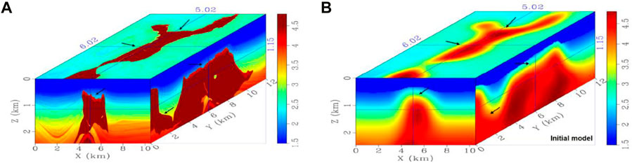
FIGURE 5. (A) 3D SEAM true velocity model. (B) 3D SEAM initial velocity model for FWI.

As a first step, the TV-regularized isotropic FWI with salt flooding is applied to produce and preserve the top of the salt body. Figure 6A shows an inverted velocity model after 30 iterations. Compared with the initial velocity model in Figure 5B, after TV regularization and the automated salt flooding, the shape of the salt (especially the top of the salt) is mostly recovered. However, most of the detailed structures are still missing, such as the clear water bottom and sedimentary layers. Therefore, an anisotropic FWI based on the new q-P approximation equation is applied for higher frequency iterations. To reduce the computational time, we only update a specific area of the SEAM model. The inversion result after anisotropic FWI is shown in Figure 6B and compared with the inverted velocity update after TV regularization and salt flooding as shown in Figure 6A, more detailed fine-layered structures below the water bottom line and at deeper parts are delineated, as circled out in Figure 6B.

FIGURE 6

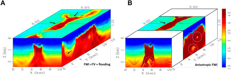
FIGURE 6. (A) Updated velocity model using 2 Hz of dominant frequency. The shape of the salt (especially the top of the salt) is recovered using regularized FWI. (B) Velocity model after salt flooding. Compared with the inverted velocity update after TV regularization, most of the salt body has been recovered.

Finally, a cross-section in the middle of SEAM is illustrated in Figure 7, the inverted model is shown in Figure 7B, and more detailed fine-layered structures at deeper parts are delineated, compared with the initial model, which is shown in Figure 7A. Figure 7C shows the true velocity model as a benchmark. The inverted and true velocity models match with each other quite well. Moreover, two validation wells (well A and well B) are demonstrated in the true model for further validation of our methodology. Figure 8 shows the comparison between initial, inverted, and true velocity models for both wells A and B, where the blue curve denotes the initial velocity and the curve in red denotes the inverted velocity. The inverted velocity model matches with the true velocity model, especially in well B, and our inversion reaches a precision of 0.986 in well B.

FIGURE 7

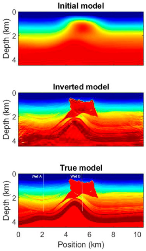
FIGURE 7. Initial model, inverted model, and true model. As can been seen, the shapes of the salt as well as detailed layered structures are well inverted compared with the true velocity model. Two validation wells are also demonstrated in the true model.

FIGURE 8

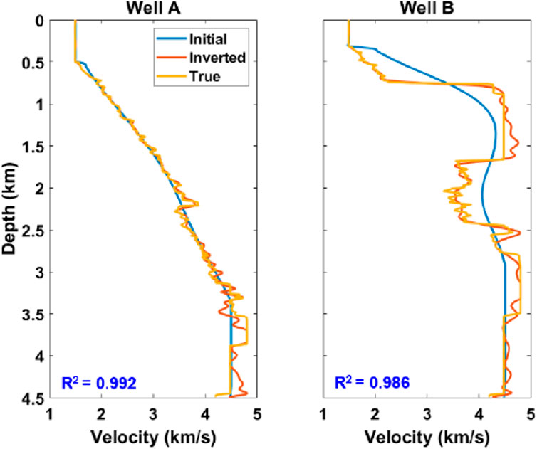
FIGURE 8. Initial and inverted velocity model comparison of two validation wells. The blue curve denotes the initial velocity, and the red curve denotes the inverted velocity. As can be seen, the inverted velocity model matches with the true velocity model.

3.2 Field data example

For the real data example, a marine seismic dataset acquired in a region of Gulf of Mexico (GOM) is applied. The area is divided into three distinct tectonic regions: compressional, extensional, and salt-dominated. The data are recorded using a short streamer of length 4.8 km. The lowest usable frequency in the dataset is approximately 6 Hz. We consider the model of interest to be 18 km × 22 km × 8 km deep. Figure 9A shows the velocity model acquired from tomography, in which the salt body is well demonstrated; however, some detailed structures are not well recovered. In that case, we will just use its salt as the reference salt body for our FWI procedure. We first smooth the velocity model to destroy the salt shape, as shown in Figure 9B. The water layer velocity is kept unchanged throughout the inversion scheme.

FIGURE 9

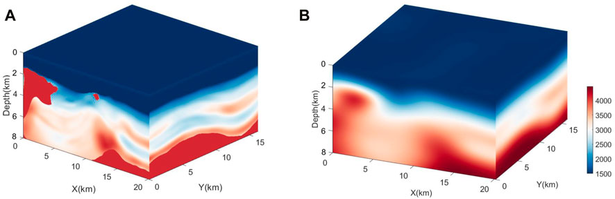
FIGURE 9. (A) Velocity model acquired from tomography, in which the salt body is well demonstrated, whereas some detailed structures are yet to be recovered. (B) Initial model for 3D FWI.

Furthermore, we start the inversion from 6 Hz (due to the lack of low-frequency data) up to 12 Hz, and the final inverted velocity model is shown in Figure 10. Compared with the initial model, the shapes of the salt body have been well updated. In addition, some detailed layered structures are also recovered. For this field data example for FWI, it is noted in the inverted model that the bottom of the salt might not be well captured. The ability of the inversion model to correct the velocity below the salt hinged on the availability of long model wavenumber updates capable of reversing the flooding. In this dataset, the lack of low frequencies and the limited available offsets contributed to this limitation.

FIGURE 10

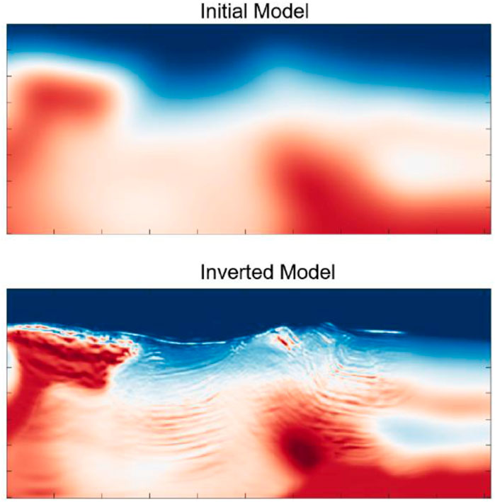
FIGURE 10. Initial model and final inverted velocity model. Compared with the initial model, the shapes of the salt body have been well updated. In addition, some detailed layered structures are also recovered.

4 Conclusion

In this study, we proposed a regularizing anisotropic FWI by penalizing the velocity drops with depth. For the first stage, we apply a regularized isotropic FWI (‘FWI + TV′) to match the low-frequency data, so as to preserve the top and sharp edges of the salt body. For the second stage, an automated flooding is applied to flood from the top of the salt to recover the deeper parts of the salt body. After the salt body is mostly recovered, the final stage that applies anisotropic TTI FWI using higher-frequency bands is used to invert more detailed structures. This split approach is extremely convenient because it is easy to implement in existing FWI schemes. This procedure is mathematically more robust and less cumbersome than the standard “migrate-pick-flood” method. Furthermore, the ‘TTI FWI′ ensures the delineating of subtle detailed structures near the salt body. We have shown the application of the proposed method to parts of the 3D SEAM model, in which the lowest available frequency of the observed synthetic datasets is 2 Hz. In addition to synthetic examples, this study has considered a challenging field dataset to invert for salt provinces.

Data availability statement

The data analyzed in this study is subjected to the following licenses/restrictions: The field datasets analyzed for this study solely belong to PETRONAS and cannot be made publicly available for legal or ethical reasons. Requests to access these datasets should be directed to junxiao.li@petronas.com.my.

Author contributions

JL and HR contributed to the conception and design of the study. JL contributed to anisotropic FWI and field data processing and wrote the first draft of the manuscript. MK and HR contributed to 3D TV and automated flooding. KX contributed to the cycle-skipping research. FD contributed to synthetic data application. HR, JL, and KX contributed to manuscript revision and read, and approved the submitted version.

Acknowledgments

The authors would like to thank PETRONAS for providing permission to show seismic/well data from the Malay basins and allowing the publication of this work.

Conflict of interest

Authors JL, HR, and FD were employed by the company PETRONAS Research Sdn Bhd, Exploration Technology, Group Research and Technology; author MK was employed by the company S-Cube; and author KX was employed by the company CNPC BGP.

Publisher’s note

All claims expressed in this article are solely those of the authors and do not necessarily represent those of their affiliated organizations, or those of the publisher, the editors, and the reviewers. Any product that may be evaluated in this article, or claim that may be made by its manufacturer, is not guaranteed or endorsed by the publisher.

References

Alkhalifah, T. (2014). Full waveform inversion in an anisotropic world: Where are the parameters hiding? EAGE Publications.

Google Scholar

Anagaw, A. Y., and Sacchi, M. D. (2012). Edge-preserving seismic imaging using the total variation method. J. Geophys. Eng. 9 (2), 138–146. doi:10.1088/1742-2132/9/2/138

CrossRef Full Text | Google Scholar

Araya-Polo, M., Jennings, J., Adler, A., and Taylor, D. (2018). Deep-learning tomography. Lead. Edge 37 (1), 58–66. doi:10.1190/tle37010058.1

CrossRef Full Text | Google Scholar

Berthelot, A., Solberg, A. H. S., and Gelius, L-J. (2013). Texture attributes for detection of salt. J. Appl. Geophys. 88, 52–69. doi:10.1016/j.jappgeo.2012.09.006

CrossRef Full Text | Google Scholar

Borisov, D., and Singh, S. C. (2015). Three-dimensional elastic full waveform inversion in a marine environment using multicomponent ocean-bottom cables: A synthetic study. J. Int. 201, 1215–1234. doi:10.1093/gji/ggv048

CrossRef Full Text | Google Scholar

Brenders, A. J., and Pratt, R. G. (2007). Full waveform tomography for lithospheric imaging: Results from a blind test in a realistic crustal model. Geophys. J. Int. 168 (1), 133–151. doi:10.1111/j.1365-246x.2006.03156.x

CrossRef Full Text | Google Scholar

Chapman, C. H., and Pratt, R. G. (1992). Traveltime tomography in anisotropic media: Theory. Geophys. J. Int. 109, 1–19. doi:10.1111/j.1365-246x.1992.tb00075.x

CrossRef Full Text | Google Scholar

Chavent, G., Clément, F., and Gómez, S. (1994). “Automatic determination of velocities via migration-based traveltime waveform inversion: A synthetic data example,” in SEG technical program expanded abstracts 1994 (Society of Exploration Geophysicists), 1179–1182.

Google Scholar

Esser, E., Guasch, L., Herrmann, F. J., and Warner, M. (2016). Constrained waveform inversion for automatic salt flooding. Lead. Edge 35 (3), 235–239. doi:10.1190/tle35030235.1

CrossRef Full Text | Google Scholar

Farmer, P., Miller, D., Pieprzak, A., Rutledge, J., and Woods, R. (1996). Exploring the subsalt: Oilfield review, 8.

Google Scholar

Farquharson, C. G. (2008). Constructing piecewise-constant models in multidimensional minimum-structure inversions. Geophysics 73 (1), K1–K9.

CrossRef Full Text | Google Scholar

Jing, Z., Zhang, Y., Chen, Z., and Li, J. (2007). “Detecting boundary of salt dome in seismic data with edge detection technique,” in 2007 SEG annual meeting (OnePetro).

Google Scholar

Jones, I. F. (2012). Tutorial: Incorporating near-surface velocity anomalies in pre-stack depth migration models. First Break 30, 47–58. doi:10.3997/1365-2397.2011041

CrossRef Full Text | Google Scholar

Kalita, M., Kazei, V., Choi, Y., and Alkhalifah, T. (2019). Regularized full-waveform inversion with automated salt flooding. Geophysics 84 (4), R569–R582. doi:10.1190/geo2018-0146.1

CrossRef Full Text | Google Scholar

Lailly, P. (1984). The seismic inverse problem as a sequence of before stack migration: Conference on inverse scattering: Theory and application, 206–220.

Google Scholar

Leeuwen, T., and Herrmann, F. J. (2013). Mitigating local minima in full-waveform inversion by expanding the search space. Geophys. J. Int. 195, 661–667. doi:10.1093/gji/ggt258

CrossRef Full Text | Google Scholar

Li, J., Xin, K., and Dzulkefli, F. S. (2022). A new qP-wave approximation in tilted transversely isotropic media and its reverse time migration for areas with complex overburdens. Geophysics 87 (4), S237–S248. doi:10.1190/geo2021-0433.1

CrossRef Full Text | Google Scholar

Luo, Y., and Schuster, G. T. (1991). Wave-equation traveltime inversion. Geophysics 56 (5), 645–653. doi:10.1190/1.1443081

CrossRef Full Text | Google Scholar

Martins, C. M., Williams, A., Lima, V. C. B., and Silva., J. C. (2011). Total variation regularization for depth-to-basement estimate: Part 1—mathematical details and applications. Geophysics 76 (1), I1–I12. doi:10.1190/1.3524286

CrossRef Full Text | Google Scholar

McCann, D., Comas, A., Martin, G., McGrail, A., and Leveille, J. (2012). Seismic data processing empowers interpretation: A new methodology serves to mesh processing and interpretation. Hart’s E&P.

Google Scholar

Michell, S., Shen, X., Brenders, A., Dellinger, J., Ahmed, I., and Fu, K. (2017). “Automatic velocity model building with complex salt: Can computers finally do an interpreter's job?,” in 2017 SEG international exposition and annual meeting (OnePetro).

CrossRef Full Text | Google Scholar

Pan, W., Innanen, K. A., Margrave, G. F., Fehler, M. C., Fang, X., and Li, J. (2016). Estimation of elastic constants for HTI media using Gauss-Newton and full-Newton multiparameter full-waveform inversion. Geophysics 81 (5), R275–R291. doi:10.1190/geo2015-0594.1

CrossRef Full Text | Google Scholar

Pan, W., Innanen, K. A., and Yu, G. (2018). Elastic full-waveform inversion and parametrization analysis applied to walk-away vertical seismic profile data for unconventional (heavy oil) reservoir characterization. Geophys. J. Int. 213, 1934–1968. doi:10.1093/gji/ggy087

CrossRef Full Text | Google Scholar

Pratt, R. G., Shin, C., and Hick, G. (1998). Gauss–Newton and full Newton methods in frequency–space seismic waveform inversion. Geophys. J. Int. 133, 341–362. doi:10.1046/j.1365-246x.1998.00498.x

CrossRef Full Text | Google Scholar

Rudin, L. I., Stanley, O., and Fatemi., E. (1992). Nonlinear total variation based noise removal algorithms. Phys. D. nonlinear Phenom. 60 (1-4), 259–268. doi:10.1016/0167-2789(92)90242-f

CrossRef Full Text | Google Scholar

Rusmanugroho, H., Li, J., Daniel Davis Muhammed, M., and Sun, J. (2022). “3D velocity model building based upon hybrid neural network,” in SEG/AAPG international meeting for applied geoscience & energy (OnePetro).

CrossRef Full Text | Google Scholar

Shen, X., Ahmed, I., Brenders, A., Dellinger, J., Etgen, J., and Scott, M. (2017). “Salt model building at Atlantis with full-waveform inversion,” in SEG technical program expanded abstracts 2017 (Society of Exploration Geophysicists), 1507–1511.

CrossRef Full Text | Google Scholar

Shin, C., and Min, D-J. (2006). Waveform inversion using a logarithmic wavefield. Geophysics 71 (3), R31–R42. doi:10.1190/1.2194523

CrossRef Full Text | Google Scholar

Tarantola, A. (1984). Inversion of seismic reflection data in the acoustic approximation. Geophysics 49, 1259–1266. doi:10.1190/1.1441754

CrossRef Full Text | Google Scholar

Vogel, C. R., and Oman, M. E. (1998). Fast, robust total variation-based reconstruction of noisy, blurred images. IEEE Trans. image Process. 7 (6), 813–824. doi:10.1109/83.679423

PubMed Abstract | CrossRef Full Text | Google Scholar

Wang, P., Zhang, Z., Mei, J., Lin, F., and Huang, R. (2019). Full-waveform inversion for salt: A coming of age. Lead. Edge 38 (3), 204–213. doi:10.1190/tle38030204.1

CrossRef Full Text | Google Scholar

Wang, Z., Hegazy, T., Long, Z., and AlRegib, G. (2015). Noise-robust detection and tracking of salt domes in postmigrated volumes using texture, tensors, and subspace learning. Geophysics 80 (6), WD101–WD116. doi:10.1190/geo2015-0116.1

CrossRef Full Text | Google Scholar

WuLuo, R. J., and Wu, B. (2014). Seismic envelope inversion and modulation signal model. Geophysics 79, WA13–WA24. doi:10.1190/geo2013-0294.1

CrossRef Full Text | Google Scholar

Zhang, Z., Mei, J., Lin, F., Huang, R., and Wang, P. (2018). “Correcting for salt misinterpretation with full-waveform inversion,” in 88th Annual International Meeting SEG, Expanded Abstracts, 1143–1147. doi:10.1190/segam2018-2997711.1

CrossRef Full Text | Google Scholar