 Christoph Marty
 Mario B. Rohrer2,3
 Matthias Huss
- 1WSL Institute for Snow and Avalanche Research SLF, Davos, Switzerland
- 2Meteodat GmbH, Zürich, Switzerland
- 3Institute for Environmental Sciences, University of Geneva, Geneva, Switzerland
- 4Laboratory of Hydraulics, Hydrology and Glaciology (VAW), ETH, Zürich, Switzerland
- 5Swiss Federal Institute for Forest, Snow and Landscape Research WSL, Zürich, Switzerland
- 6Department of Geosciences, University of Fribourg, Fribourg, Switzerland
Snowpack is an important temporal water storage for downstream areas, a potential source of natural hazards (avalanches or floods) and a prerequisite for winter tourism. Here, we use thousands of manual measurements of the water equivalent of the snow cover (SWE) from almost 30 stations between 1,200 and 2,900 m a.s.l. from four long-term monitoring programs (earliest start in 1937) in the center of the European Alps to derive daily SWE based on snow depth data for each station. The inferred long-term daily SWE time series were analyzed regarding spatial differences, as well as potential temporal changes in variability and seasonal averages during the last 7 decades (1957–2022). The investigation based on important hydro-climatological SWE indicators demonstrates significant decreasing trends for mean SWE (Nov-Apr) and for maximum SWE, as well as a significantly earlier occurrence of the maximum SWE and earlier disappearance of the continuous snow cover. The anomalies of mean SWE revealed that the series of low-snow winters since the 1990s is unprecedented since the beginning of measurements. Increased melting during the accumulation period below 2000 m a.s.l is also observed–especially in the most recent years–as well as slower melt rates in spring, and higher day-to-day variability. For these trends no regional differences were found despite the climatological variability of the investigated stations. This indicates that the results are transferable to other regions of the Alps.
1 Introduction
Monitoring the water equivalent of the snow cover (SWE) has a long history in snow-dominated regions like the Swiss Alps (Haberkorn, 2019), which can be seen climatically as a representative subset of the core of the European Alps (Matiu et al., 2021). The measurement of SWE was born from the need to know the amount of water stored in the snowpack, because–from a hydro-meteorological perspective–snow is just temporally frozen precipitation. Three important questions were and still are in focus: 1) the amount of precipitation at high elevations, 2) the influence of forest on the snowpack, and 3) the amount of water stored in the snow cover in relation to the total precipitation. The answers to these three questions are important for understanding water runoff variability or glacier dynamics. Today it is clear that there are three basic properties used to describe the snow cover–snow depth, bulk snow density, and snow water equivalent–and they are interconnected with each other by the fact that bulk density together with snow depth determines the SWE. Snow depth is by far the simplest and therefore most frequently measured and analyzed parameter. On the other hand, measurements of SWE or snow density are either costly or time-consuming and, hence, typically sparse. However, these parameters influence the thermal, mechanical, and optical properties of snow. Data of SWE and/or snow density are therefore indispensable for snow-related research and its applications. In Switzerland four different SWE monitoring programs, each with its own history, have evolved during the last century and are still operational today.
1) Glaciers: End-of-winter SWE measurements on about a dozen of Swiss glaciers, of which we here analyze the series of two fixed point sites on Claridenfirn.
2) Wägital: Catchment-based SWE measurements based on snow courses, originally for water resource monitoring.
3) Nation-wide: In-situ SWE measurements at two dozen of stations mainly reporting for daily snow- and avalanche observations.
4) Alptal: In-situ SWE measurements for the long-term investigation of forest-snow interactions at multiple sites, of which we here analyze the only complete series available.
During the last decades data from these different monitoring programs have been used for the development of the national snow load code (Martinec, 1975), forest-snow interactions (López-Moreno and Stähli, 2008), international snow model inter-comparisons (Rutter et al., 2009), microwave backscattering of snow (Werner et al., 2010), snow climate projections (Schmucki et al., 2014), international solid precipitation inter-comparisons (Smith et al., 2017), snow model development (Wever et al., 2015; Fiddes et al., 2019), snow density parametrizations (Jonas et al., 2009; Helfricht et al., 2018; Guidicelli et al., 2021), glacier mass-balance investigations (Huss et al., 2021) and sensor tests (Stähli et al., 2004; Steiner et al., 2019; Capelli et al., 2022). However, each of these studies has always only used data from one of these individual monitoring programs, and a joint analysis is still missing, possibly due to the different temporal resolution of the measurements.
The goal of this investigation is therefore to show the history and similarities of the different SWE monitoring programs in Switzerland and to demonstrate that the different programs, spanning a large elevation range and topographical characteristics, have a common denominator which enables us to use a merged dataset for climatological purposes. We therefore present the first intercomparison of the variability and trends of long-term SWE time series from these four different data sources.
In the next section, the general measurement procedure of manual SWE data, which is the base of all four monitoring programs, is first described (Section 2.1). Second, the four data sets and their history are introduced (Section 2.2). Third, the methods to derive daily time series from temporally irregular SWE measurements are presented (Section 2.3). Fourth, the used hydro-climatological SWE indicators, on which the main analysis is based on, are defined (Section 2.4). Finally, the applied statistical methods are described (Section 2.5).
2 Methods and data
2.1 Manual measurement of water equivalent of the snow cover
The general procedure for the determination of in-situ SWE is to use snow-core samplers, which are inserted vertically from the top surface into the snowpack. Samplers with teeth need to be twisted, while those with sharpened rims only need to be twisted in very dense snow. Depending on the design, samples can only be excavated with a snow pit (hereafter called cylinder samplers) or without digging a snow pit (hereafter called tube samplers). A graduation on the sampler is used to determine the height of the sample of known diameter and therefore known volume. A scale is used to measure the weight of the sample. The density of each such measurement sample can then be calculated by dividing the weight by the volume. The water equivalent of this sample is found by multiplying the density with the height of the sample. When the snowpack is deeper than the length of the sampler, measurements need to be repeated until the ground surface is reached. To separate one measurement level from the next, the application of a thin plate is favorable. Finally, point-scale SWE can be calculated by adding up the water equivalent of the different samples. Otherwise, bulk density can be calculated by dividing the found SWE by total snow depth.
Regarding the determination of SWE at a measurement station, it is important to note that the measured SWE always must be related to snow depth at a permanently installed snow measuring stake as the SWE measurement itself is a destructive measurement method. This means that the snow depth at the location of the SWE measurement usually does not correspond to the snow depth at the stake because neither the ground nor the snow cover surface is perfectly level. The same is true in the case of so-called snow courses, where the SWE of a larger area is inferred by taking many snow depth measurements but only a few bulk density measurements. In both cases, the bulk snow density at the spot of the SWE measurement is calculated by dividing SWE by the height(s) of the probed snow sample(s). Since this bulk snow density is much less variable in space than snow depth (Korhonen, 1932; López-Moreno et al., 2013), final SWE for an area or a measurement station can be calculated by multiplying the bulk snow density with the snow depth, ideally measured at a daily interval at a fixed stake in the measurement field.
2.2 Data sets
The main characteristics and differences of the four different monitoring programs are described in the next sub-sections and are listed in Table 1. The used Claridenfirn data consists of two once-a-year (usually May) measurements at two locations (2,680 and 2,890 m), both starting in 1914 for snow depth, both only with complete SWE records since 1957. The Wägital data are based on once-a-year (April 1) acquired snow density and snow course measurements, which are spatially interpolated for the entire catchment (900–2,300 m), starting in 1943. The largest share of the measurements stems from the national snow and avalanche observation network, which is maintained by the institute for snow and avalanche research (SLF) and are henceforth referred to as SLF stations. These twice-a month, station-based measurement series were mainly started in the 1940s and are located between 1,200 and 2,500 m. The Alptal data are based on once-a-week SWE measurements at one location at 1,210 m starting in 1969. With the exception of the Claridenfirn measurements (see Section 2.2.1) the method to determine SWE has not changed since the beginning of monitoring. The stations used form the four different SWE monitoring programs are listed in Table 2 and geographically visualized in Figure 1.

TABLE 1. Main characteristics and differences between each of the four independent SWE measurement programs.
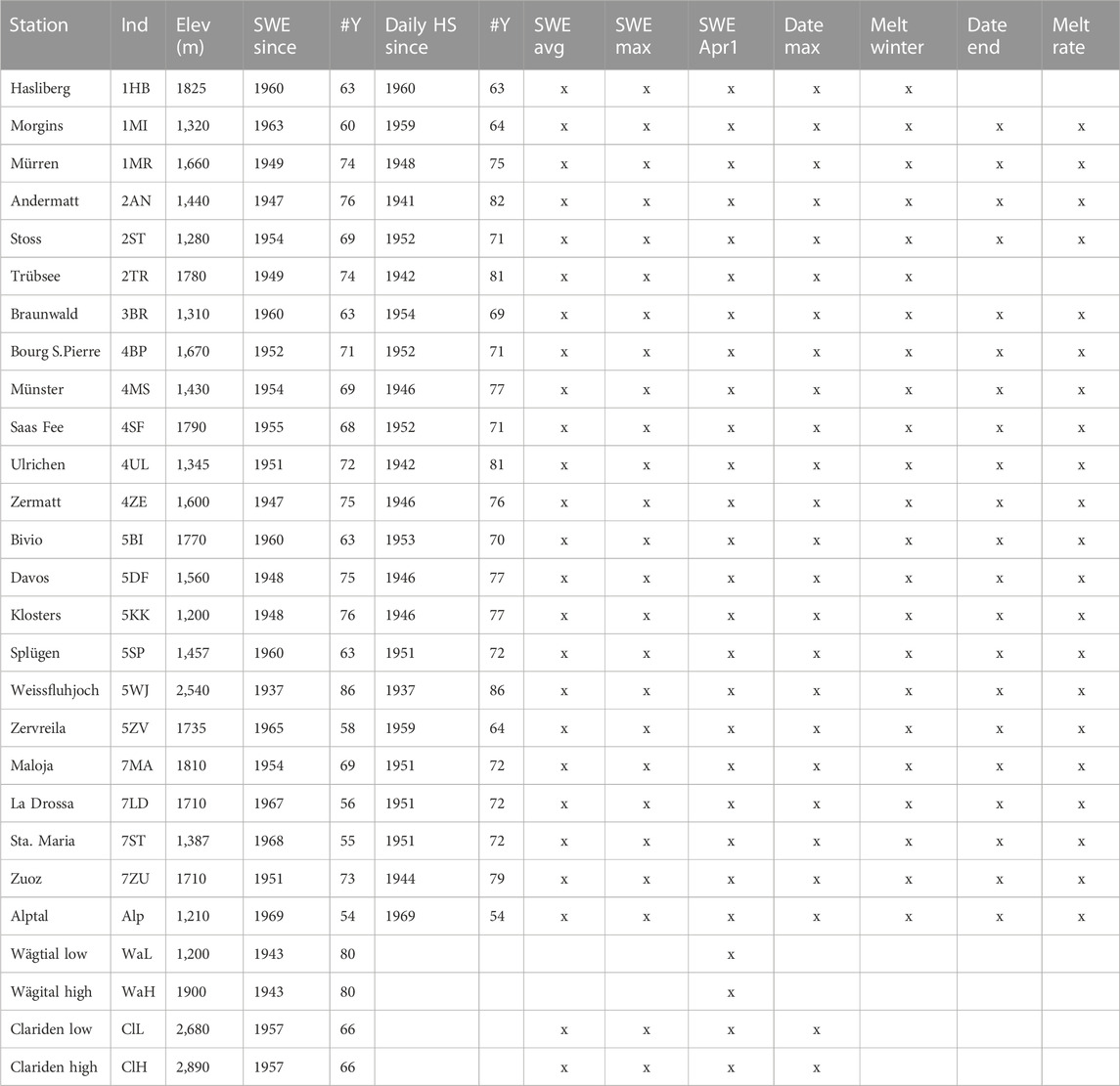
TABLE 2. Long-term stations used for the analysis and corresponding length (#Y) of SWE and daily snow depth (HS) time series available. The distribution of the available length of the SWE series is given in Figure 1 as boxplot. The definition of the SWE indicators given in the last seven columns is given in Table 3.
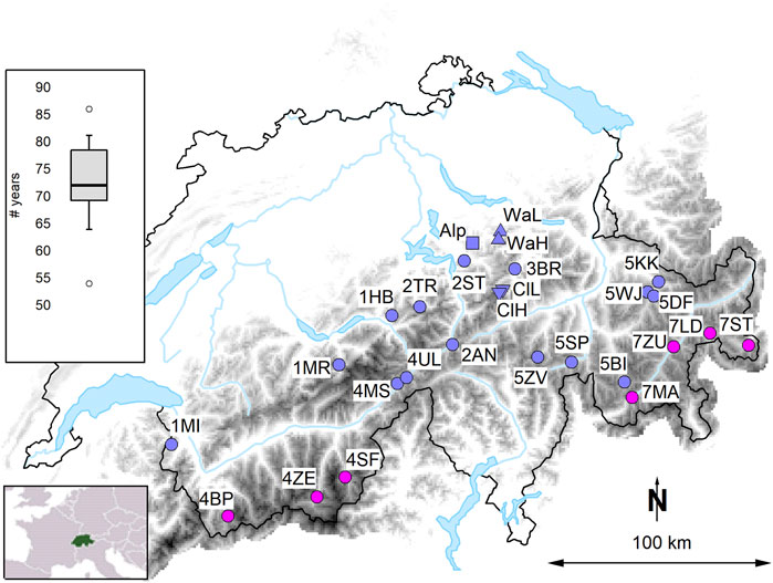
FIGURE 1. Spatial distribution of all 27 long-term stations. Stations are colored based on climatologies mainly influenced by the weather of northern (purple) or their location in inner-alpine dry valleys (pink) along the main Alpine divide (Figure 3). Locations of the national snow and avalanche network (SLF stations) are represented by circles, the Wägital time series as up-pointing triangles, the Claridenfirn measurements by down-pointing triangles and the Alptal data by a square. Elevations above 1,000 m a.s.l. are given in gray-scaled shading in the background. The location of Switzerland within Europe is shown in the lower left corner. The distribution of the length of the available time series is provided as boxplot in the upper left corner.
2.2.1 Glacier mass-balance measurements on claridenfirn
End-of-winter snow depth (HS) and SWE are currently determined on 15 Swiss glaciers at 1–5 sites per glacier with detailed snow density measurements, and snow courses consisting of 30–300 additional HS measurements to determine the SWE averaged over the entire glacier. Even though some of these observational series extend over 100 years, only the observations performed at two locations on Claridenfirn, Eastern Switzerland, have a completeness and consistency necessary to be included in the present study. Claridenfirn is a mountain glacier in north-eastern Switzerland with an area of 4.3 km2 (2019) and an elevation range from 2,550 to 3,250 m a.s.l. over mostly gentle surface slopes. The long-term monitoring program consist of two individual mass-balance time series at point locations at current elevations of 2,890 and 2,680 m a.s.l., respectively (see Supplementary Material S1.1.2).
Such end-of-winter snow depth measurements are available since 1914. End-of-winter SWE measurements are however only available since 1957. These point-scale SWE determination, i.e., bulk density measurements are accomplished at the end of the accumulation period typically in May to determine the winter mass balance (winter SWE). Measurements are performed at or close to stakes drilled into the firn or ice. Stakes permit a direct measurement of the firn/ice layer thickness gain/loss. Until spring 2018 the bulk density has been determined by digging a snow pit down to the layer of last summer’s snow level marked with ochre or sawdust (from the end of summer mass balance measurements) and measuring the SWE with the 55 cm long cylindric ETH-sampler (see Supplementary Material S1.1.3). Since spring 2019 the bulk snow density is determined with the help of a self-designed firn drill with a 86 mm inner diameter.
There is no year since 1957 in which the observation of winter SWE is missing for both stations at the same time. It is however missing for 28% of the years at the lower site and only for 5% at the upper site. When no density observation was available, the long-term mean bulk density was used to convert snow/firn depth to SWE. Missing direct bulk density observations for winter SWE at the lower site are restricted to the period before 1979 (Müller and Kappenberger, 1991; Huss and Bauder, 2009).
2.2.2 Snow water resource measurements in the wägital catchment
The catchment-wide SWE investigations in the Wägital described in this sub-section and the SWE measurements at SLF stations (next sub-section) were originally initiated for water resource monitoring by the same founder but are now fully separated (see additional details in Supplementary Material S1.1.3). The Wägital measurement series started at the beginning of April 1943. SWE measurements were accomplished at several locations within the Wägital catchment, which situated in the NE-Prealps of the Swiss Canton of Schwyz. This catchment extends from 900 to ca. 2,300 m a.s.l. and has an area of 42.35 km2.
For the estimation of SWE for the entire catchment area, snow densities and snow depths are measured at 10 specific locations, while snow depths alone are additionally measured along 28 snow courses, each with between 10 and 30 measurements. These different measurements are acquired at representative locations, that are considered characteristic for a certain altitude and exposure, and are accessible for in-situ measurements without the risk of avalanches. To determine SWE in the field, snow pits are dug each spring and snow samples are taken using the ETH sampler described earlier. The bulk snow density for each measurement location is then calculated. This measurement procedure is carried out since the beginning in 1943, always around April 1st, which typically is the time when the peak SWE occurs in the upper part of the catchment.
By interpolating the snow densities for each 100 m elevation zone and main exposures, a function is fitted in every year. Based on this function and the respective snow depth measurements, the snow mass is estimated for each elevation zone and main exposure. By integrating the snow mass values over altitude and exposition zones, the water equivalent for the entire catchment area can be calculated. To evaluate possible elevation-dependent differences, the catchment-wide snow mass has been separated into two elevations bands (lower band 900–1,500 m a.s.l.: 24.68 km2, upper band 1,500–2,300 m a.s.l.: 13.49 km2). The two SWE series used in this study are derived by dividing the spatial snow mass of each elevation zone by the corresponding area. Thereby creating two virtual stations, with the corresponding mean elevation of 1,200 m a.s.l.for the lower zone and 1900 m a.s.l.to the higher zone. Further details about the catchment, measurement efforts and the data can be found in Noetzli and Rohrer (2014).
2.2.3 Nation-wide SWE measurements at SLF stations
The fact that SLF snow and avalanche observers look into the snowpack to investigate the snow stratigraphy was used to also measure SWE in the same pit (see Supplementary Material S1.1.4). These measurements are typically acquired in a seasonally fenced flat measurement field that is 15 by 15 m in size. Daily measurements of snow depth are conducted each morning by reading the value from a fixed stake with a centimeter scale. SWE measurements are taken twice-a-month (mid and end of each month) as long as there is at least 10 cm of snow on the ground along a so-called profile line. These stations are typically located at the valley floor between 1,200 and 1800 m a.s.l. The only exception is the measurement field at Weissfluhjoch (2,540 m), which is situated in the middle of a ski area.
The number of such stations with twice-a-month SWE measurements has increased from 10 stations in the 1940s to around 45 stations after the 1990s. In the first decade of the new millennium, the number of stations slightly decreased, but this decline was halted thanks to the growing demand for SWE measurements as verification points for flood forecasting models. Unfortunately, as with any other monitoring network, some long-term measurement series had to be abandoned during the last 7 decades due to a lack of observer availability or funding. Nevertheless, at least 22 series, which began in the 1960s or earlier, have a duration of at least 50 years.
2.2.4 Forest-snow interaction investigations in the alptal valley
The Alptal forest-snow interaction site is situated in the NE-Prealps, just 18 km west of the Wägital catchment. Manual SWE measurements are currently made at 15 locations representing different elevations, slope exposures and vegetation types (see Supplementary Material S1.1.5). For this study, however, we only use data from the longest available measurement series in an open meadow, which started in 1969. It is a west-exposed, open meadow measurement field located close to the Erlenhöhe meteorological station at an elevation of 1,220 m. SWE is measured with custom-made tube sampler of 5 cm inner diameter and 120 cm length, at irregular intervals that range from 1 week to 1 month. Snow depth is measured automatically with ultrasonic sensor since winter 2002/03. Prior to this winter, daily snow depth values are available from the numerical model COUP. Details about the measurement site, the data and the applied model can be found in Stähli and Gustafsson (2006).
2.3 Derivation of daily SWE data
To compare the temporally irregular SWE measurements from the different monitoring programs the DeltaSnow model (Winkler et al., 2021) is used. This model converts measured HS to daily SWE values using individually calibrated coefficients for each monitoring station. The DeltaSnow model is preferred because it requires only daily snow depth data as input, which was already available as quality-check and complete time series at all but four of the stations. The model calculates SWE based on accumulation, compaction and drenching of an indefinite series of snow layers using seven parameters that need to be calibrated. These parameters were determined separately for each station by using long-term measured SWE values for calibration. The DeltaSnow model performs very well in modeling the temporal evolution of SWE on the daily scale, with a low level of uncertainty as shown by Winkler et al. (2021) and confirmed by Fontrodona-Bach et al. (2023). After the station-based calibration, the model demonstrates a RMSE of 30 mm (5%–10%) and a mean bias of 1 mm (Aschauer et al., 2023). It is important to note that the uncertainty of the model must be viewed in the context of the uncertainty of the SWE measurements of about 10%–15% (López-Moreno et al., 2020).
Moreover, the alternative, i.e., comparing raw measurements directly would also introduce uncertainties for inter-stations comparisons, as the SWE observation at the middle and the end of each month usually differs by ± 2 days from the target date, which implies a possible difference between the actual measurement date of up to 5 days, i.e., up to a third of the typical measurement interval. The use of the regularly measured HS data as basis has additional benefits. Firstly, the few winters with missing SWE data (only one to three winters at half of the stations, the other half was complete) could easily be filled. Secondly, since the measurement of snow depth started often earlier than the SWE measurements, the timeseries could be prolonged by a few years. Finally, data of only one winter at one station (5BI) was still missing since this station also had no HS measurement in 1964. This gap was filled by using data of the best correlated neighboring station (Aschauer and Marty, 2021).
Two of the four above mentioned stations without daily HS values were the two measurement locations on Claridenfirn. These twice-a-year measurements at the end of the accumulation season (median date May 26) and at end of the ablation season (median date September 25) are used to constrain a snow accumulation and degree-day melt model to derive daily SWE series for the two stake locations (Huss et al., 2021). The model was fitted to the two measurement values per year and the variability in between these two dates was determined by meteorological input from a nearby station. More information about the used data and the general measurement uncertainty of point mass-balance series is provided in Huss et al. (2021). The other two series without daily HS measurements come from the Wägital catchment, where SWE is only measured once per year on April 1, and no additional HS measurements are available throughout the season. Therefore, this is the only case where the temporal evolution of daily SWE values could not be derived.
2.4 Data availability, SWE indicators and climatology
The SWE measurements from the above-described different monitoring programs (Figure 1) finally led to complete timeseries of 27 measurement stations with a total of 1968 station winters (Table 1). The stations are located between 1,200 and 2,900 m asl, with most stations between 1,200 and 1800 m. Unfortunately, there are no stations between 2000 and 2,500 m a.s.l.– and only three stations above 2,500 m. The spatial distribution of the available stations is heavily biased towards the north of the main Alpine divide (Figure 1). In fact, there is only one station (7ST) south of the Alpine divide. The length of the timeseries varies between 54 and 86 years, with a median of 72 years. The data is investigated based on hydrological years. For this study, the hydrological year is defined as the 12 months between September 1 and August 31.
Based on the hypotheses that the increasing temperatures have an impact on SWE we decided to investigate different SWE indicators for each station, which are illustrated in Figure 2 and defined in Table 2. The indicator SWEAvg is based on the average SWE between November 1 and April 30 as this is the main snow-covered period for most of the timeseries and ephemeral snow before and after this period is often not measured. SWEApr1 indicator is often used a proxy for the date of peak SWE (SWEMax) for non-glacierized locations (Bohr and Aguado, 2001), and it is also the long-term measurement date for the Wägital monitoring program. In contrast, SWEMax, DateMax (date of SWEMax) and DateEnd (date of disappearance of the continuous snow cover) are based on the longest snow-covered period. In case of two equal periods, the latter is taken. To provide additional snow-hydrological information the following cumulative indicators MeltWinter and MeltRate have been derived: MeltWinter is the sum of daily melt (decrease in SWE) between November 1 and DateMax (accumulation period) and MeltRate is the average melt per day calculated between DateMax and DateEnd (ablation period).
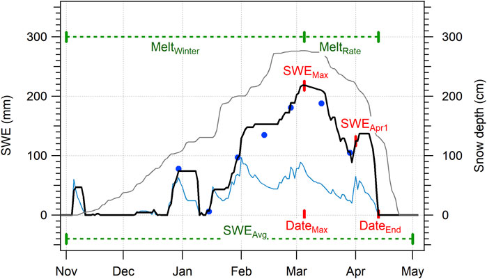
FIGURE 2. Example of the daily evolution of modeled SWE (black line) and the twice a month measured SWE (blue dots) at a station at 1,350 m a.s.l. The long-term mean SWE evolution is illustrated with a grey line. The corresponding daily measured snow depth (right axis) is shown in blue. The SWE indicators related to 1 day are given in red, indicators calculated over a certain measurement period are given in green.
For comparability reasons with the large majority of all other (non-glacierized) stations MeltWinter, DateEnd and MeltRate was not used for the two glacier stations on Claridenfirn (ClL and ClH) as sometimes not all snow does melt, which implicates that there is no actual start and end date of the continuous snow cover within a hydrological year. Similarly, DateEnd and MeltRate could not be calculated for the two stations 1HB and 2TR, both located in ski areas, because there is not always staff available during the late melt season (May and June). Moreover, for the two timeseries in the Wägital catchment due to missing daily HS measurements only the indicator SWEApr1 could be calculated (see Section 2.3).
2.5 Climatology and trend analysis
To identify potential climatological differences between the various stations being investigated, mean values and their variability [standard deviation and the coefficient of variation (CV)] have been calculated for each time series between November and April. To be able to intercompare the temporal evolution of the SWE series with different absolute magnitudes, the relative deviation from the long-term average of each time series has been determined. For this purpose, the 30-year average between 1991 and 2020 (standard reference period) is calculated for every station and the absolute difference between the annual values and 30-year average is determined and normalized by the 30-year average.
To analyze possible long-term changes, we applied the non-parametric Mann–Kendall (MK) test, which is based on rank-transformed time series, where only the relative magnitude of the measurement is considered (Mann, 1945). A positive standardized MK value indicates an increasing trend, while a negative value demonstrates a decreasing one. Confidence levels of 99% are used as a threshold to classify a highly significant trend (p < 0.01), confidence levels of 95% (p<0.05) are defined as medium significant and confidence levels of 90% are used to classify a weakly significant trend (p<0.1).
For the detection of the timing of trend turning points and occurrence of significance, the sequential version of the MK test was applied (Sneyers, 1992). The strength of a trend was determined with a robust simple linear regression with the Theil–Sen slope estimator (Sen, 1968). Absolute trends were calculated as decadal changes, while relative trends were calculated as percentage changes between 1957 and 2022 based on the Theil-Sen slope. We chose to begin our analysis in 1957, as only four station time series have missing years before the beginning of the measurements (one station 12 years, or 18% and the other three stations either two or 3 years). It is important to note that a direct comparison of percentage changes is only meaningful between indicators of the same unit and similar absolute values.
3 Results
3.1 Climatology and variability
Climatological mean values and their variability for the reference period 1991–2020 are shown in dependence of elevation for all stations in Figure 3. All stations along the main Alpine divide (i.e., located in inner-alpine valleys, see Figure 1) clearly show lower mean values and higher CVs than the remaining stations, especially for SWEAvg, SWEMax and SWEApr1.
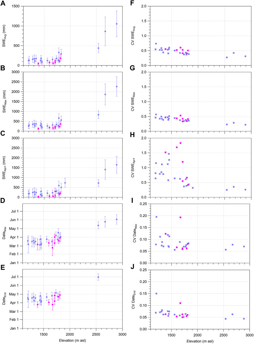
FIGURE 3. (A–E) Climatological mean values and their standard deviation for the reference period 1991–2020, as well as (F–J) corresponding Coefficients of Variation (CV). Stations that are located in inner-alpine valleys along the main Alpine divide (see Figure 1) are marked in pink, all other stations are marked in purple.
SWEAvg values vary between about 50 mm for the only station on the south side of the Alpine ridge and 1,000 mm for the highest station whereas SWEMax values vary between 100 mm and 2,200 mm for the same two stations. The large majority of stations (situated between 1,200 and 1800 m) show mean values around 150 mm and max values around 350 mm. SWEApr1values are generally slightly lower and show distinctively higher CVs than all other SWE indicators. SWEMax is generally reached between March 1 and April 1 for stations below 1700 m. The few stations between 1700 and 2,900 m a.s.l. experience SWEMax between April 1 and June 1.
DateEnd occurs between April 1 and May 1 for most of the stations below 1900 m. The only station available at higher elevation (at 2,540 m) usually becomes snow-free at the beginning of July. Both DateMax and DateEnd show a remarkably low temporal spread.
While all indicators increase with elevation, values below 1700 m a.s.l. remain remarkably stable. In contrast, the CVs of SWEMean, SWEMax and SWEApr1 show decreasing values with elevation across the entire elevation range.
3.2 Long-term trends
In contrast to average values, long-term trends of all SWE indicators show no clear elevation dependence (Figure 4). However, five of the seven investigated indicators demonstrate clear trends for most of the stations. The strongest signal is seen in the date of disappearance of SWE, with a significant decreasing trend (DateEnd being earlier) observed at almost 80% of the stations. More than half of the stations also show significant decreasing trends for SWEAvg and DateMax. In addition, somewhat more than 40% of the stations show significant decreasing trends for SWEMax. Trends in SWEApr1 are not shown, because they are similar to the trends in SWEMax, but with only 20% of stations being significant. These trends are plotted in Supplementary Figure S1 to illustrate that there are no clear spatial differences depending on the regional setting of the stations.
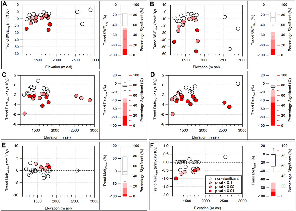
FIGURE 4. Absolute (left) long-term decadal trend of the indicators SWEAvg (A), SWEMax (B), DateMax (C), DateEnd (D), MeltWinter (E) and MeltRate (F) in dependence of station elevation. The color of the circles represents the significance of the trend. Relative Trends over the entire investigation period 1957–2022 (right) are given as boxplots (with the 25%, respectively 75% percentiles representing the box and the 10%, respectively 90% percentiles representing the whiskers) and the percentage of significant stations (at various significance levels) is shown as bar graphs.
SWEAvg values are mostly decreasing by between 5 and 20 mm/10 y (median = 8 mm/10 y), whereas SWEMax is mostly decreasing by between 5 and 30 mm/10 y (median = 13 mm/10 y). Trends in the date of maximum SWE (DateMax) indicate that SWEMax shift towards earlier dates by 1–3 days/10 years (median = 1.9 days/10 y), whereas the date of snow disappearance (DateEnd) show an even stronger decadal trend (median =2.5 days/10 y) towards earlier time in the year. In contrast to all other indicators, DateMax and DateEnd also reveals significant changes for the few stations above 2000 m a.s.l.
Regarding the indicator MeltWinter, 25% of the stations display weak but significant trends, with all of them being positive ranging between 1 and 3 mm/10 y. These positive trends are found only among stations located between 1,400 and 1800 m. The remaining stations either display positive trends (13%), no trend (42%), or slightly negative trends (20%), but none of these trends are significant according to the MK-test applied. Similarly, for the indicator MeltRate, 25% of the stations exhibit weak but significant trends, which are all negative with values ranging between 0.5 and 1 mm/10 y. This suggests a slight decrease in the rate of snow melt towards the end of the snow-cover season. The remaining stations show negative but insignificant trends (21%), no trend (45%), or slightly positive trends (9%).
Upon closer examination using the sequential MK-test, it becomes clear that there is little evidence of a long-term trend in SWE indicators until the late 1980s. Since then, trends begin to emerge towards decreasing SWEAvg, SWEMax, MeltRate and simultaneously increasing MeltWinter as well as earlier DateMax, DateEnd. This development is particularly well illustrated in Figure 5, which shows the relative anomalies of all stations for SWEAvg. The median of all stations reveals a 30% decrease during the investigated period, which is significant at a 96% (p =0.04), consistent with the −35% decrease shown in Figure 4A. The same comparison is provided in Table 3 for all SWE indicators, hence corroborating the findings of Figure 4 and revealing the relative changes (although non-significant) also for two indicators MeltWinter and MeltRate.
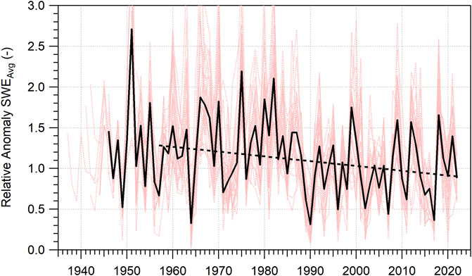
FIGURE 5. Relative anomaly in SWEAvg with respect to the period 1991–2020 for all investigated stations (light red lines). The black line indicates the median of all stations. A clear evolution is revealed (black dotted line from Theil-Sen estimation) despite the number of stations and local climates involved. The median is not shown before 1946, because only five stations are available before this year and the trend is shown for the main investigated period between 1957 and 2022.
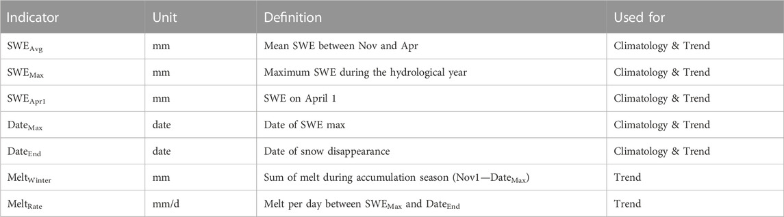
TABLE 3. Definition and units of the SWE indicators used.
4 Discussion
4.1 Mean values and variability
The intercomparison of the complete data set consisting of results from different monitoring programs, was only made possible by using daily data derived through modeling constrained with the observations. The daily model shows small biases at all stations, which can be attributed to the multi-decadal time span covered by the SWE measurements allowing for individual calibration for each time series.
Overall, Figures 3A–E shows a clear increase of all SWE indicators (except DateEnd) with elevation. However, a closer look reveals an absence of an elevation-dependence below 1700 m a.s.l. that is mainly caused by non-further increasing values above 1,400 m a.s.l. This can be explained by the fact that the few stations between 1,400 and 1700 m a.s.l. are located in inner-alpine valleys, which are rather snow-scarce due to the precipitation shading effect of surrounding mountains.
The analysis of these climatological mean values of the investigated SWE indicators confirms that the stations along the main Alpine divide get lower snow amounts, experience earlier DateMax and DateEnd due to their protected location in inner-alpine valleys, which are relatively dry (Matiu et al., 2021). However, these stations are sometimes also influenced by humid airflow from the Mediterranean Sea in the south. The switch between these two weather states is responsible for the generally higher CVs (Figures 3F–J) observed at these stations for SWEAvg, SWEMax and SWEApr1. This is not the case for the CVs of DateMax and DateEnd, i.e., the start and the end of the snow ablation season. The timing and intensity of the ablation season is primarily driven by positive temperatures in spring, whose variability does not differ north and south of the Alps.
The CVs of the SWE indicators mentioned above exhibit a clear elevation dependence, with decreasing CVs at higher elevations. This pattern arises because the variability in snow mass at low elevation is dominated by the combined variability of temperature and precipitation, whereas at high elevation the snow mass is mainly dominated by precipitation (Morán-Tejeda et al., 2013; Marty et al., 2017). The by far highest CV values are found for SWEApr1 at stations located below 1700 m. This is because this indicator reflects the state of just 1 day, which can be snow-abundant (e.g., after a major snowfall event) or already snow-free after the first spring warming. These finding are consistent with previous studies (Kapnick and Hall, 2010) which suggest that SWE on April 1 is not a reliable indicator for long-term snow hydrological investigations.
4.2 Long-term trends
The temporal evolution of SWE (Figure 5) with a strongly decreasing trend at the end of the 1980s and a flattening of the trend after about 2007 is known from many temperature-dominated processes (Reid et al., 2015). The stable conditions of SWE until the 1980s have already been reported by Rohrer et al. (1994) for Alpine measurement sites in Switzerland. The relative anomalies of the SWEAvg reveal a regime shift after 1988, as indicated by Marty (2008) for snow-cover days in Switzerland and confirmed by Colombo et al. (2022) for snow water equivalent in the Italian Alps. This late 1980s abrupt temperature change coincided with abrupt hydroclimatic changes and is consistent with circulation variability and long-term warming (Sippel et al., 2020). It is evident that snowfall depends on precipitation and temperature. However, studies have shown that–below about 2,500 m a.s.l.—on the long-term and for the most recent decades, temperature is the dominating factor for the amount and duration of snow on the ground (Scherrer et al., 2004; Colombo et al., 2022). This is especially the case in Switzerland, where no precipitation trend but a strong increase in temperature could be observed during winter in the recent decades (Isotta et al., 2019).
The most significant trends over the entire elevation range were observed for DateEnd, which is mostly temperature-driven (Table 4). This finding is supported by the fact that air temperature during snow melt (spring temperature) increased more than in the winter season in the Alps (Isotta et al., 2019). Klein et al. (2016) also found a significant trend for DateEnd of 5.8 days/10 y, which is double the trend revealed in our study (2.5 days/10 y). The reason for this difference is the fact that our study investigates more than twice as many stations and covers a longer time period (1957–2022 vs. 1975–2015).
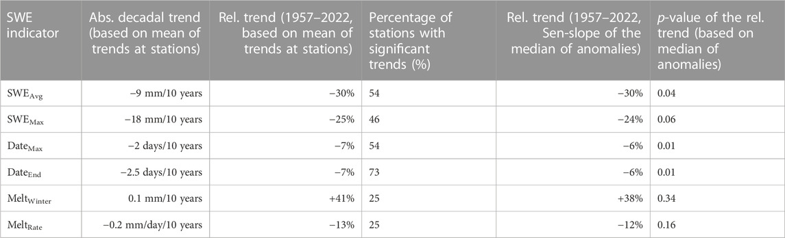
TABLE 4. Comparison of magnitude and significance of trends for individual SWE indicators (first three columns, see also Figure 4), and trends calculated based on the Sen-slope of the median of the anomalies of the individual stations (last two columns, see also Figure 5).
The higher absolute trends of SWEMax compared to SWEAvg need to be interpreted in relation to the absolute values. Relative trends (1957–2022) show smaller values for SWEMax (median = −25%) compared to SWEAvg (median = −35%), which is consistent with other studies comparing mean and maximum snow depth values in Europe (Fontrodona Bach et al., 2018; Matiu et al., 2021).
The observations that SWEAvg and SWEMax decline, as well as the earlier occurance of maximum SWE (DateMax) and SWE disappearance (DateEnd) are indications that the melt sum during the accumulation season (MeltWinter) have increased over time (especially below 2000 m). This is not surprising given the rise in winter temperatures and the corresponding shift from more snowfall days to more rain days (Serquet et al., 2011). Moreover it is in agreement with similar findings from western North America (Musselman et al., 2021).
However, there is a large year-to-year and the inter-station variability of the MeltWinter indicator. Therefore, it is not surprising that the annual median values demonstrate an insignificant (p=0.13) increase of 1.3 mm/10 y (Figure 6). Moreover, this is consistent with the results found for the individual stations in Figure 4E, where only 25% of the stations demonstrated a significant increase. Most striking is the series of winters with a large melt sum after 2015. When analyzing the observed increase of the MeltWinter indicator it must be noted that this is a measure for snow mass loss. However, before actual snow mass loss is happening and, in addition to periods with snow mass loss, there must be many days where melt just happens on the top or in the snowpack, and subsequent refreezing of the melt water, without a net mass loss. Additional and preceding periods of such a wetting and warming of the snowpack (Birsan et al., 2005; Petersky et al., 2019) are not reflected with our MeltWinter indicator. Moreover, since DateMax is moving closer towards November, the potential number of melt days are also slightly decreasing. Therefore, the observed increase of MeltWinter is rather a conservative measure for the increased wetting of the snowpack—especially considering the fact that the applied DeltaSnow model used to retrieve daily SWE cannot capture rain-on-snow events, which have become more frequent in recent decades (Beniston and Stoffel, 2016). The observed increase in wetting of the snowpack is also in line with indications to more wet snow avalanches in mid-winter (Pielmeier et al., 2013) and projections of more wet snow earlier in the season (Castebrunet et al., 2014).
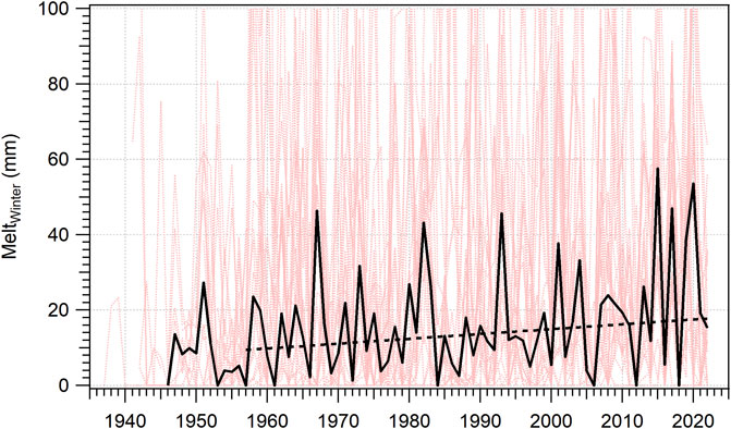
FIGURE 6. Time series of the summed snow melt between November 1 and the date of maximum SWE (MeltWinter). The median of all station is shown with the black line and the corresponding Sen slope (black dotted line) is given between 1957 and 2022. Original annual values of all individual stations are in the background (light red). Median values are not shown before 1946, because only five stations are available before this year.
The combination of higher amounts of melting during the accumulation season and the earlier onset of the ablation period (which increases the chance for snowfall after DateMax) in the most recent decades are responsible for an increase in the day-to-day variability of SWE (Figure 7), expressed as coefficient of variation based on the daily SWE data. The median of the increase at individual stations reveals a positive trend of 17% between 1957 and 2022. Higher stations (i.e., usually snow-rich stations) are affected much less by these two processes because temperatures are generally cold enough to prevent significant melting in the accumulation season and are often already warm enough after the DateEnd to usually prevent snowfall thereafter.
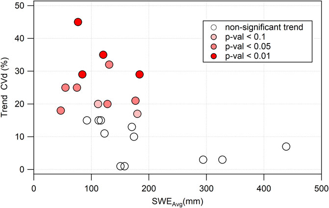
FIGURE 7. Relative trend between 1957–2022 of the SWE day-to-day variability (CVd) in dependence of SWEAvg of each station. Significant trends are colored in red.
The above-described process during the accumulation season also contributes to a higher occurrence of short snow-cover periods before the onset of the continuous snow cover. Since the observed changes indicate that stations at higher elevation are increasingly adopting the characteristics of lower stations, the long-term increase in day-to-day SWE variability is consistent with the larger day-to-day variability seen at lower stations compared to higher stations. It is important to note that the day-to-day variability should not be confused with the year-to-year SWE variability shown in Figure 3F. A separate investigation based on decadal changes of this year-to-year variability revealed a non-significant increase (+21% during the study period between 1957 and 2022) according to the MK test. This is in line with the observed pattern that the year-to-year SWE variability at lower (generally warmer) stations is higher than at higher (generally colder) stations (Figure 3F).
The absence of a general elevation-dependence for the calculated trends of the SWE indicators (Figure 4) can be explained by the following facts: First, the available stations are all located above the mean winter zero degree line (900 m a.s.l.), which means the impact is small despite warming temperatures. Moreover, the warming above 900 m is weak during the accumulation (i.e., winter) season compared to the other seasons (Isotta et al., 2019). No clear elevation signal was also demonstrated in a larger snow depth dataset covering the entire Alps (Matiu et al. (2021). Second, all indicators except SWEAvg have a time-dependent component that affects the trends if the time period of snow ablation is shifted closer (higher solar radiation) or further from the summer solstice (lower solar radiation). SWEAvg is also the only indicator, which indicates an elevation-dependence for the relative trend (Figure 8) with smaller decreases for higher elevations.
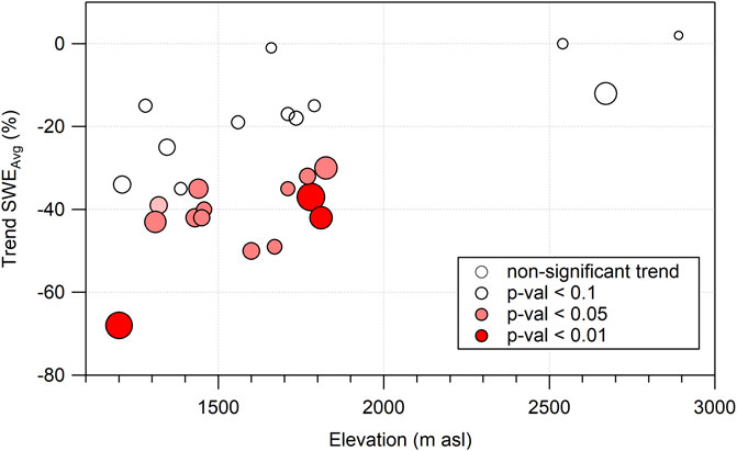
FIGURE 8. Relative trend (1957–2022) of SWEAvg in dependence of elevation. The significance of the trend is in indicated by the red colors. The size of the circles represents the magnitude of the absolute trend between 3 and −26 mm per decade (see Figure 4A).
Regarding the decreasing MeltRate observed at stations below 2000 m a.s.l. during the ablation season (Figure 4F) the proximity to the summer solstice is also relevant. Lower melt rates are caused by an earlier start of the ablation period, i.e., by a shift of DateMax (Figure 4C) from about end of March to mid-March, when there is less energy for melt available. This finding is consistent with other studies that found generally lower melt rates in a warmer climate (Musselman et al., 2017). However, this does not apply for the highest station, which demonstrates increasing MeltRate (Figure 4F), because the earlier DateEnd (Figure 4D) is moving their ablation period closer to summer solstice.
Furthermore, the wetting of the snowpack and the decreasing snow mass as well as the increased variability, have significant consequences on hydrology, ecology, and tourism. For example, rain-on-snow events can lead to floods as the dampening effect of an already wet snow cover is strongly reduced. The shift to more winter melt may sustain microbial activity and thus accelerate the carbon production in the cold season (Williams et al., 2015), but it can also put plant species at risk if they are unable to adapt to more erratic snow-hydrological regimes (Rixen et al., 2022). Additionally, earlier snow disappearance may impact streamflow droughts with corresponding impacts downstream (Jenicek et al., 2016; Brunner et al., 2023). Lastly, changes in snowpack can also impact tourism. For instance, a wetting of the snowpack means less “powder days” (i.e., less days with fresh, light snow), which are highly valued by skiers and therefore often promoted by ski areas.
The studied SWE indicators and, hence, the main results of this study are model based, but they were informed and constrained with actual measurements of daily snow depth. Comparisons with daily measured SWE timeseries revealed a high performance of DeltaSnow in modelling daily SWE dynamics and peak SWE occurrence if used with regional calibration parameters (Fontrodona-Bach et al., 2023). This performance is even better when station-based calibration is possible as shown in Aschauer et al. (2023). Additionally, independent experiences based on a separate analysis of some Swiss investigation sites corroborated the high capability of DeltaSnow to model the accurate timing and magnitude of daily SWE changes (see Supplementary Figure S2).
5 Conclusion
For the first time, the merging of long-term SWE measurements series of four individual monitoring programs in the Swiss Alps distributed over an extensive elevation range allowed a comprehensive analysis of trends and variability of these indicators. All the investigated stations provide exceptional SWE measurement series spanning more than 6 decades (1957–2022) allowing for investigating long-term changes in important hydro-climatological snow indicators.
It could be shown that results of the four monitoring programs encompassing a large elevation range from forest to glaciers are in good agreement with each other and can well be inter-compared despite different backgrounds and measurement protocols. The analysis confirmed, for example, that the often-used SWE on April 1 is not a good indicator for trend analysis as the year-to-year variability is much higher than for other indicators like annual maximum SWE. The clearest trends were found for a shift of the date of snow disappearance towards earlier in the season (−2.5 days/10 y), mean SWE during the winter season (−9 mm/10 y), and the date of maximum SWE (−2 days/10 y). More than half of the stations showed significant trends for these three indicators. The anomalies of mean SWE revealed that the last 3 decades is the only period since beginning of measurements in 1937, with such a cluster of snow scarce winters. Maximum SWE also demonstrated a clear decreasing trend (−18 mm/10 y) with slightly less than half of the stations being significant, but with a median decrease of almost 120 mm (−25%) during the 66 years under investigation. This decrease of maximum SWE even for the highest stations has a significant impact on the summer discharge downstream in large rivers with corresponding implications to many other sectors.
Significant positive trends for melting during the accumulation period and significant negative shifts in the melt rate during the ablation period were observed for about a quarter of the investigated stations only. However, it is important to note that there is a general increasing trend for winter melting (+38% between 1957 and 2022, no station shows a significant decreasing trend) and a general decreasing trend in melt rates (−12% between 1957 and 2022, no station shows a significant increasing trend). These findings reveal that significant snow hydro-climatological changes are also occurring during the longer accumulation season and not just during the comparably short ablation season.
The increase in winter melting implies more wet snow (wetting does happen even more without snow mass loss due to refreezing) during accumulation phase of the snowpack. The thus caused snow mass loss during the accumulation season contributes to the observed occurrence of earlier and smaller maximum SWE values. Additionally, short-term melting events, which cause snow mass loss are also mainly responsible for the observed 17% increase in the variability of the day-to-day SWE changes between 1957 and 2022.
Finally, the presented results reveal that the changes in snow-hydrological processes predicted by climate models can already be confirmed with long-term observations of the snow cover. This underscores the importance of long-term monitoring programs in advancing snow-climatological modeling efforts. To better understand and project the combined impacts of increased melting during the accumulation season and higher variability in snow amounts on different sectors, more high-quality measurements of SWE and meteorological data in snow-dominated mountain regions are crucial.
Data availability statement
The datasets presented in this study can be found in online repositories. The names of the repository/repositories and accession number(s) can be found below: Data from the Wägital catchment are available from: https://doi.org/10.5281/zenodo.6473327. Data from the SLF observer network are available from: https://doi.org/10.16904/15. Data from the Alptal measurement series are available from: https://www.envidat.ch/dataset/longterm-hydrological-observatory-alptal-central-switzerland Data from Claridenfirn are available from: https://doi.glamos.ch/data/massbalance_point/massbalance_point_2022_r2022.html, and https://doi.glamos.ch/pubs/intrep/intrep_1.html, daily data are available on request.
Author contributions
CM and MR conceptualized the overall study. MR, MH, and MS provided data and information on the Wägital, Claridenfirn and Alptal data sets, respectively. CM did most of the analysis and wrote the first draft of the manuscript, while all authors contributed to the final version of the paper. All authors contributed to the article and approved the submitted version.
Funding
During the last 7 decades the four different monitoring programs were mostly funded by the institutions which maintained the measurements during that time. In the last decade, except for the Alptal measurements, all other long-term monitoring programs were partly funded by MeteoSwiss in the framework of GCOS Switzerland. This study was also partly financed by MeteoSwiss in the framework of GCOS Switzerland. Open access funding by Swiss Federal Institute for Forest, Snow and Landscape Research (WSL).
Acknowledgments
We are grateful for the above-mentioned support of MeteoSwiss in the framework of GCOS Switzerland and for the initiation of this study. The decade-long measurements of all four monitoring programs relied on many snow observers, scientists, technicians, or student helpers. We thank Andreas Bauder (VAW ETH) for sharing his in-depth knowledge regarding historic measurement methods on the Claridenfirn and we acknowledge the support of Johannes Aschauer for providing the station dependent DeltaSnow coefficients. We are also grateful to Dylan Reynolds and Charles Fierz for their invaluable assistance with proofreading and streamlining this manuscript with their expertise.
Conflict of interest
Author MR was employed by the company Meteodat GmbH.
The remaining authors declare that the research was conducted in the absence of any commercial or financial relationships that could be construed as a potential conflict of interest.
Publisher’s note
All claims expressed in this article are solely those of the authors and do not necessarily represent those of their affiliated organizations, or those of the publisher, the editors and the reviewers. Any product that may be evaluated in this article, or claim that may be made by its manufacturer, is not guaranteed or endorsed by the publisher.
Supplementary material
The Supplementary Material for this article can be found online at: https://www.frontiersin.org/articles/10.3389/feart.2023.1165861/full#supplementary-material
References
Aschauer, J., and Marty, C. (2021). Evaluating methods for reconstructing large gaps in historic snow depth time series. Geosci. Instrum. Method. Data Syst. 10, 297–312. doi:10.5194/gi-10-297-2021
Aschauer, J., Michel, A., Jonas, T., and Marty, C. (2023). An empirical model to calculate snow depth from daily snow water equivalent: SWE2HS 1.0, Geosci. Model Dev. 2023, 1–19. doi:10.5194/gmd-2022-258
Beniston, M., and Stoffel, M. (2016). Rain-on-snow events, floods and climate change in the Alps: Events may increase with warming up to 4°C and decrease thereafter. Sci. Total Environ. 571, 228–236. doi:10.1016/j.scitotenv.2016.07.146
Birsan, M.-V., Molnar, P., Burlando, P., and Pfaundler, M. (2005). Streamflow trends in Switzerland. J. Hydrology 314, 312–329. doi:10.1016/j.jhydrol.2005.06.008
Bohr, G. S., and Aguado, E. (2001). Use of April 1 SWE measurements as estimates of peak seasonal snowpack and total cold-season precipitation. Water Resour. Res. 37, 51–60. doi:10.1029/2000WR900256
Brunner, M. I., Götte, J., Schlemper, C., and Van Loon, A. F. (2023). Hydrological drought generation processes and severity are changing in the Alps. Geophys. Res. Lett. 50, e2022GL101776. doi:10.1029/2022GL101776
Capelli, A., Koch, F., Henkel, P., Lamm, M., Appel, F., Marty, C., et al. (2022). GNSS signal-based snow water equivalent determination for different snowpack conditions along a steep elevation gradient. Cryosphere 16, 505–531. doi:10.5194/tc-16-505-2022
Castebrunet, H., Eckert, N., Giraud, G., Durand, Y., and Morin, S. (2014). Projected changes of snow conditions and avalanche activity in a warming climate: The French Alps over the 2020-2050 and 2070-2100 periods. Cryosphere 8, 1673–1697. doi:10.5194/tc-8-1673-2014
Colombo, N., Valt, M., Romano, E., Salerno, F., Godone, D., Cianfarra, P., et al. (2022). Long-term trend of snow water equivalent in the Italian Alps. J. Hydrology 614, 128532. doi:10.1016/j.jhydrol.2022.128532
Fiddes, J., Aalstad, K., and Westermann, S. (2019). Hyper-resolution ensemble-based snow reanalysis in mountain regions using clustering. Earth Syst. Sci. 23, 4717–4736. doi:10.5194/hess-23-4717-2019
Fontrodona Bach, A., van der Schrier, G., Melsen, L. A., Klein Tank, A. M. G., and Teuling, A. J. (2018). Widespread and accelerated decrease of observed mean and extreme snow depth over Europe. Geophys. Res. Lett. 45 (12), 312. doi:10.1029/2018GL079799
Fontrodona-Bach, A., Schaefli, B., Woods, R., Teuling, A. J., and Larsen, J. R. (2023). Purification of the secondary treatment tail water for wastewater reclamation by integrated subsurface-constructed wetlands. Earth Syst. Sci. Data Discuss. 2023, 1–9. doi:10.1080/09593330.2023.2176260
Guidicelli, M., Gugerli, R., Gabella, M., Marty, C., and Salzmann, N. (2021). Continuous spatio-temporal high-resolution estimates of SWE across the Swiss Alps – a statistical two-step approach for high-mountain topography. Front. Earth Sci. 9. doi:10.3389/feart.2021.664648
Haberkorn, A. (2019). European snow booklet – An inventory of snow measurements in Europe. EnviDat. doi:10.16904/envidat.59
Helfricht, K., Hartl, L., Koch, R., Marty, C., and Olefs, M. (2018). Obtaining sub-daily new snow density from automated measurements in high mountain regions. Hydrol. Earth Syst. Sci. 22, 2655–2668. doi:10.5194/hess-22-2655-2018
Huss, M., and Bauder, A. (2009). 20th-century climate change inferred from four long-term point observations of seasonal mass balance. Ann. Glaciol. 50, 207–214. doi:10.3189/172756409787769645
Huss, M., Bauder, A., Linsbauer, A., Gabbi, J., Kappenberger, G., Steinegger, U., et al. (2021). More than a century of direct glacier mass-balance observations on Claridenfirn, Switzerland. J. Glaciol. 67, 697–713. doi:10.1017/jog.2021.22
Isotta, F. A., Begert, M., and Frei, C. (2019). Long-term consistent monthly temperature and precipitation grid data sets for Switzerland over the past 150 years. J. Geophys. Res. Atmos. 124, 3783–3799. doi:10.1029/2018JD029910
Jenicek, M., Seibert, J., Zappa, M., Staudinger, M., and Jonas, T. (2016). Importance of maximum snow accumulation for summer low flows in humid catchments. Earth Syst. Sci. 20, 859–874. doi:10.5194/hess-20-859-2016
Jonas, T., Marty, C., and Magnusson, J. (2009). Estimating the snow water equivalent from snow depth measurements in the Swiss Alps. J. Hydrology 378, 161–167. doi:10.1016/j.jhydrol.2009.09.021
Kapnick, S., and Hall, A. (2010). Observed climate–snowpack relationships in California and their implications for the future. J. Clim. 23, 3446–3456. doi:10.1175/2010JCLI2903.1
Klein, G., Vitasse, Y., Rixen, C., Marty, C., and Rebetez, M. (2016). Shorter snow cover duration since 1970 in the Swiss Alps due to earlier snowmelt more than to later snow onset. Clim. Change 139, 637–649. doi:10.1007/s10584-016-1806-y
López-Moreno, J. I., Fassnacht, S. R., Heath, J. T., Musselman, K. N., Revuelto, J., Latron, J., et al. (2013). Small scale spatial variability of snow density and depth over complex alpine terrain: Implications for estimating snow water equivalent. Adv. Water Resour. 55, 40–52. doi:10.1016/j.advwatres.2012.08.010
López-Moreno, J. I., Leppänen, L., Luks, B., Holko, L., Picard, G., Sanmiguel-Vallelado, A., et al. (2020). Intercomparison of measurements of bulk snow density and water equivalent of snow cover with snow core samplers: Instrumental bias and variability induced by observers. Hydrol. Process. 34, 3120–3133. doi:10.1002/hyp.13785
López-Moreno, J. I., and Stähli, M. (2008). Statistical analysis of the snow cover variability in a subalpine watershed: Assessing the role of topography and forest interactions. J. Hydrology 348, 379–394. doi:10.1016/j.jhydrol.2007.10.018
Marty, C. (2008). Regime shift of snow days in Switzerland. Geophys. Res. Lett. 35. Artn L12501. doi:10.1029/2008gl033998
Marty, C., Tilg, A.-M., and Jonas, T. (2017). Recent evidence of large-scale receding snow water equivalents in the European Alps. J. Hydrometeorol. 18, 1021–1031. doi:10.1175/jhm-d-16-0188.1
Matiu, M., Crespi, A., Bertoldi, G., Carmagnola, C. M., Marty, C., Morin, S., et al. (2021). Observed snow depth trends in the European Alps: 1971 to 2019. Cryosphere 15, 1343–1382. doi:10.5194/tc-15-1343-2021
Morán-Tejeda, E., López-Moreno, J. I., and Beniston, M. (2013). The changing roles of temperature and precipitation on snowpack variability in Switzerland as a function of altitude. Geophys. Res. Lett. 40, 2131–2136. doi:10.1002/grl.50463
Müller, H., and Kappenberger, G. (1991). Claridenfirn-Messungen 1914-1984: Daten und Ergebnisse eines gemeinschaftlichen Forschungsprojektes. Verlag d. Fachvereine1991.
Musselman, K. N., Addor, N., Vano, J. A., and Molotch, N. P. (2021). Winter melt trends portend widespread declines in snow water resources. Nat. Clim. Change 11, 418–424. doi:10.1038/s41558-021-01014-9
Musselman, K. N., Clark, M. P., Liu, C., Ikeda, K., and Rasmussen, R. (2017). Slower snowmelt in a warmer world. Nat. Clim. Change 7, 214–219. doi:10.1038/nclimate3225
Noetzli, C., and Rohrer, M. (2014). Schneemessungen in alpinen Einzugsgebieten im Zeichen des Klimawandels. Wasser Energ. Luft 106.
Petersky, R. S., Shoemaker, K. T., Weisberg, P. J., and Harpold, A. A. (2019). The sensitivity of snow ephemerality to warming climate across an arid to montane vegetation gradient. Ecohydrology 12, e2060. doi:10.1002/eco.2060
Pielmeier, C., Techel, F., Marty, C., and Stucki, T. (2013). “Wet snow avalanche activity in the Swiss Alps–trend analysis for mid-winter season,” in Proceedings of the international snow science workshop, grenoble and chamonix, 1240–1246.
Reid, P. C., Hari, R. E., Beaugrand, G., Livingstone, D. M., Marty, C., Straile, D., et al. (2015). Global impacts of the 1980s regime shift. Glob. Change Biol. 22 (2), 682–703. doi:10.1111/gcb.13106
Rixen, C., Høye, T. T., Macek, P., Aerts, R., Alatalo, J. M., Anderson, J. T., et al. (2022). Winters are changing: Snow effects on arctic and alpine tundra ecosystems. Arct. Sci. 8, 572–608. doi:10.1139/as-2020-0058
Rohrer, M. B., Braun, L. N., and Lang, H. (1994). Long-term records of snow cover water equivalent in the Swiss Alps: 1. Analysis. Hydrology Res. 25, 53–64. doi:10.2166/nh.1994.0019
Rutter, N., Essery, R., Pomeroy, J., Altimir, N., Andreadis, K., Baker, I., et al. (2009). Evaluation of forest snow processes models (SnowMIP2). J. Geophys. Res. D Atmos. 114, D06111. doi:10.1029/2008jd011063
Scherrer, S. C., Appenzeller, C., and Laternser, M. (2004). Trends in Swiss Alpine snow days: The role of local- and large-scale climate variability. Geophys. Res. Lett. 31, L13215 13211–13214. doi:10.1029/2004gl020255
Schmucki, E., Marty, C., Fierz, C., and Lehning, M. (2014). Evaluation of modelled snow depth and snow water equivalent at three contrasting sites in Switzerland using SNOWPACK simulations driven by different meteorological data input. Cold Reg. Sci. Tech. 99, 27–37. doi:10.1016/j.coldregions.2013.12.004
Sen, P. K. (1968). Estimates of the regression coefficient based on Kendall's tau. J. Am. Stat. Assoc. 63, 1379–1389. doi:10.1080/01621459.1968.10480934
Serquet, G., Marty, C., Dulex, J.-P., and Rebetez, M. (2011). Seasonal trends and temperature dependence of the snowfall/precipitation-day ratio in Switzerland. Geophys. Res. Lett. 38. doi:10.1029/2011gl046976
Sippel, S., Fischer, E. M., Scherrer, S. C., Meinshausen, N., and Knutti, R. (2020). Late 1980s abrupt cold season temperature change in Europe consistent with circulation variability and long-term warming. Environ. Res. Lett. 15, 094056. doi:10.1088/1748-9326/ab86f2
Smith, C. D., Kontu, A., Laffin, R., and Pomeroy, J. W. (2017). An assessment of two automated snow water equivalent instruments during the WMO Solid Precipitation Intercomparison Experiment. Cryosphere 11, 101–116. doi:10.5194/tc-11-101-2017
Sneyers, R. (1992). On the use of the statistical analysis for objective determination of climate change. Meteorol. Z. 247-256.
Stähli, M., and Gustafsson, D. (2006). Long-term investigations of the snow cover in a subalpine semi-forested catchment. Hydrol. Process. 20, 411–428. doi:10.1002/hyp.6058
Stähli, M., Stacheder, M., Gustafsson, D., Schlaeger, S., Schneebeli, M., and Brandelik, A. (2004). A new in situ sensor for large-scale snow-cover monitoring. Ann. Glaciol. 38, 273–278. doi:10.3189/172756404781814933
Steiner, L., Meindl, M., Fierz, C., Marty, C., and Geiger, A. (2019). “Monitoring snow water equivalent using low-cost GPS antennas buried underneath a snowpack,” in 2019 13th European conference on antennas and propagation (EuCAP), 1–5. 31 March-5 April 2019.
Werner, C., Wiesmann, A., Strozzi, T., Schneebeli, M., and Matzler, C. (2010). “The snowscat ground-based polarimetric scatterometer: Calibration and initial measurements from Davos Switzerland, Geoscience and Remote Sensing Symposium (IGARSS),” in 2010 IEEE international, 2363–2366. 25-30 July 2010.
Wever, N., Schmid, L., Heilig, A., Eisen, O., Fierz, C., and Lehning, M. (2015). Verification of the multi-layer SNOWPACK model with different water transport schemes. Cryosphere 9, 2271–2293. doi:10.5194/tc-9-2271-2015
Williams, C. M., Henry, H. A. L., and Sinclair, B. J. (2015). Cold truths: How winter drives responses of terrestrial organisms to climate change. Biol. Rev. 90, 214–235. doi:10.1111/brv.12105
Keywords: snow water equivalent, monitoring, European alps, climate warming, variability, measurement, DeltaSnow model
Citation: Marty C, Rohrer MB, Huss M and Stähli M (2023) Multi-decadal observations in the Alps reveal less and wetter snow, with increasing variability. Front. Earth Sci. 11:1165861. doi: 10.3389/feart.2023.1165861
Received: 14 February 2023; Accepted: 29 May 2023;
Published: 15 June 2023.
Edited by:
Nozomu Takeuchi, Chiba University, JapanReviewed by:
Jessica D. Lundquist, University of Washington, United StatesSatoru Yamaguchi, National Research Institute for Earth Science and Disaster Resilience (NIED), Japan
Copyright © 2023 Marty, Rohrer, Huss and Stähli. This is an open-access article distributed under the terms of the Creative Commons Attribution License (CC BY). The use, distribution or reproduction in other forums is permitted, provided the original author(s) and the copyright owner(s) are credited and that the original publication in this journal is cited, in accordance with accepted academic practice. No use, distribution or reproduction is permitted which does not comply with these terms.
*Correspondence: Christoph Marty, bWFydHlAc2xmLmNo