 Waqar Ali Zafar1,2
 Farhan Javed2Rizwan Ahmed1
 Muhsan Ehsan3*
 Kamal Abdelrahman4Mohammed S. Fnais4Mansoor Aziz Qureshi5
- 1Department of Nuclear Engineering, Pakistan Institute of Engineering and Applied Sciences, Islamabad, Pakistan
- 2Centre for Earthquake Studies, National Center for Physics, Islamabad, Pakistan
- 3Department of Earth and Environmental Sciences, Bahria School of Engineering and Applied Sciences, Bahria University, Islamabad, Pakistan
- 4Department of Geology and Geophysics, College of Science, King Saud University, Riyadh, Saudi Arabia
- 5Geology Department, Lund University, Lund, Sweden
The Kalabagh strike–slip fault, which is characterized by right-lateral movement, is part of the northwestern Himalayan foreland fold and thrust belt in Pakistan. This structure marks the western and eastern terminations of the Salt Range and Surghar Ranges, respectively. No significant (>M6) earthquakes have been reported along the Kalabagh Fault in recent decades. Here, we take advantage of space-borne Sentinel-1A SAR interferometry to gain insight into the mechanics of faulting, aseismic creeping, and stress loading of the seismic cycle on the Kalabagh Fault spanning over approximately 7 years. In this study, we also removed the tropospheric effects using the Generic Atmospheric Correction Online Service data from the rate map. We further resolved the LOS deformation into both horizontal and vertical deformations. Our Bayesian inversion indicates that the fault experiences significant horizontal and vertical displacements. The fault’s southern and northern segments exhibit a creeping rate of approximately ∼4.2 ± 1.3 to 4.8 ± 1.6 mm/year, respectively, while the central section does not display any horizontal creeping. We found that the creeping is confined between 0 and ∼2.7 ± 1.1 km depth at the northern section and 0 and ∼3.9 ± 1.1 km on the southern section of the faults. Nevertheless, we found that the vertical creeping of ∼10 mm/year is confined between 0.5 and 6 km depth in the central segment of the fault. Moreover, our model does not resolve the interseismic slip at depth on the Kalabagh Fault. Our results affirm that Kalabagh Fault is creeping, and the internal deformation due to the presence of a thick salt layer over the decollement facilitates the creeping on this fault. In addition, Coulomb stress modeling depicts that the creeping on the Kalabagh Fault increases the Coulomb stress changes in the northern section of the KBF.
1 Introduction
The Himalayas are the resultant of the colliding interaction of the Indian and Eurasian plates during the late Cretaceous to early Tertiary periods (Wells, 1984; Yeats et al., 1984; Yeats and Hussain, 1987; McDougall and Khan, 1990; McDougall and Hussain, 1991; Pogue et al., 1992; Smith et al., 1994; Beck et al., 1995; Jaswal et al., 1997; Yin and Harrison, 2000; Khan and Glenn, 2006). Researchers have long been intrigued by this collision product to investigate the traits that change during the earthquake cycles. Several devastating earthquakes have resulted from this collision (Abbas et al., 2022). The suture zone formed by the Indian plate subducting beneath the Eurasian plate is dominated by numerous thrusting features in the southern region (Pudsey, 1986; Pogue et al., 1992; Bender and Raza, 1995). This region has also experienced the introduction of significant strike–slip structures due to the shoulder-rubbing nature of the collision between two plates at some points (Yeats et al., 1984; Jaswal et al., 1997; Yin and Harrison, 2000; Khan and Glenn, 2006; Abbas et al., 2022). Although thrusting and folding account for the majority of the deformation in the northwest Himalayas (McDougall and Khan, 1990; McDougall and Hussain, 1991; Jaswal et al., 1997; Khan and Glenn, 2006), the existence of strike–slip motion in the area makes the region’s tectonic system challenging to comprehend. The Punjab foreland basin along the northwestern Himalayan frontal thrust system is underlain by the Salt, Surghar, and Trans Indus ranges as a result of the progressive deformation brought on by the continent–continent type of collision (Baker et al., 1988; Blisniuk et al., 1998; Chen and Khan, 2009). Due to progressive tectonic processes of thrusting and folding, known structural reentrants in the region have displayed relatively substantial lateral variation in the deformation throughout the ranges that are under the process of ongoing growth (Houseman and England, 1986; Pudsey, 1986; Yeats and Hussain, 1987; Baker et al., 1988; Pogue et al., 1992; Smith et al., 1994; Blisniuk et al., 1998). However, a deep analysis of the components that counterbalance the frontal thrust system is lacking (Chen and Khan, 2010).
A major strike–slip structure in this region is the Kalabagh Fault (Yeats et al., 1984; Baker et al., 1988; McDougall and Khan, 1990; Blisniuk et al., 1998; Chen and Khan, 2010), shown in Figure 1. This structure truncates the Salt Range on the western end (Baker et al., 1988; McDougall and Khan, 1990; Abbas et al., 2022), one of the largest salt-hosting formations in the world. This fault has been studied from different perspectives recently. Yeats et al. (1984) claimed that Ghundi underwent Quaternary deformation. Long-term displacement along the Kalabagh Fault by piercing point data was used by McDougall and Khan (1990) to compute the average slip rate. Chen and Khan calculated the slip rate in the Kalabagh Fault Zone using two descending SAR images of ERS-1 and ERS-2 satellite data in 2010. Because of the available data source constraints and the use of a single viewing geometry, Chen and Khan (2010) could only compute the slip rate in the northern section of the Kalabagh Fault. Sentinel-1A, the most recent mission of the Interferometric Synthetic Aperture Radar (InSAR), is run by the European Space Agency and provides much more precise data to evaluate the creep rate across the fault (Savage and Lisowski, 1993; Lee et al., 2003; Titus et al., 2006; Cavalié et al., 2008). Sentinel-1A provides improved uncertainty of about 1 mm/yr over 100 km and better temporal and spatial coverage (Bürgmann et al., 2000; Hsieh et al., 2011; Jolivet et al., 2012; Zheng et al., 2017; Ng et al., 2018; Rosi et al., 2018) for the estimation of the slip rates across the whole Kalabagh Fault accurately.
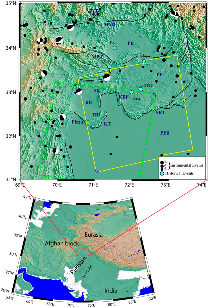
FIGURE 1. Map showing the study region, which is characterized by prominent tectonic and topographic features. The black solid circles in different sizes represent recent seismicity distribution in the area, with magnitudes ranging from 5 to 7. The focal mechanisms of the earthquakes are also shown with beach ball diagrams. The light blue circles represent historical seismicity from available records. The yellow and green rectangles demarcate the ascending (T: 173) and descending (T: 005) tracks of the Sentinel-1A radar data processed for the current investigations, respectively. The blue arrows on the rectangles show the flight (up and down) and line-of-sight (LOS) (left and right) directions of the radar on each track. The black solid lines show significant faults in the study area. Names of faults abbreviated in the map are as follows: KBF, Kalabagh Fault; KT, Khisor Thrust; TIR, Trans Indus Ranges; BB, Banu Basin; PB, Peshawar Basin; PFB, Punjab Foreland Basin; PP, Potwar Plateau; SR, Surghar Ranges; SRT, Salt Range Thrust; MMT, Main Mantle Thrust; MKT, Main Karakoram Thrust; MBT, Main Boundary Thrust; and JF, Jhelum Fault.
Numerous studies have used InSAR data successfully for comprehending transient strain accumulation (Peltzer et al., 2001; Walters et al., 2013), creeping in the San Andreas Fault (Rosen et al., 1998; Johanson and Bürgmann, 2005), and slip rates on key faults of western Tibet (Chen et al., 2018). To estimate the slip rate accurately for active faults in a given area, which typically exhibit very slow slip rates (few mm/year), InSAR measurement can be utilized due to its exceptional signal-to-noise ratio (Peltzer et al., 2001; Wright et al., 2004; Xu et al., 2016; Yu et al., 2017).
More precise measurements of deformation and slip rate along the Kalabagh Fault are necessary in addition to the existing studies to comprehend the fault behavior. Previous studies on the Kalabagh Fault also did not account for atmospheric noise in their analyses. We employed the small baseline subset (NSBAS) technique and atmospheric correction through Generic Atmospheric Correction Online Service for InSAR (GACOS) to determine the rate map. Data of both ascending and descending tracks for 7 years, from 2015 to 2022, were analyzed to ensure comprehensive coverage and minimize the effect of atmospheric noise in the estimation of slip rates. In the end, we simulated the Coulomb stress changes due to the creeping of the KBF on nearby local strike–slip and thrust faults.
2 Materials and methods
An established method for measuring ground deformation brought on by the buildup of interseismic strain is InSAR time-series analysis (Fialko, 2006; Jolivet et al., 2013; Biggs and Wright, 2020; Weiss et al., 2020). In several instances, InSAR has proven its capability to estimate as low slip rates as a few millimeters in a year (Fialko, 2006; Prati et al., 2010; Tong et al., 2013; Mousavi et al., 2015; Xu et al., 2016; Yu et al., 2017; Weiss et al., 2020). Several techniques and methodologies have been developed to compute the rate map of active fault systems (Berardino et al., 2003; Werner et al., 2003). In the current work, the deformation along the Kalabagh Fault was estimated using the SBAS–InSAR approach. This technique has significantly improved measurements of crustal deformation, for example, by establishing the spatio-temporal baseline of the chosen interferograms, which produces coherent deformation time series (Castellazzi et al., 2016). The SBAS InSAR time-series technique lessens the phase decorrelation effects by adding a filter to signals with strong spatial correlation but lower temporal correlation (Berardino et al., 2003; Hooper, 2008; Ferretti et al., 2011).
With full images of Pakistan being captured on average every 12 days, the Sentinel-1, C-band SAR satellites from the European Space Agency (ESA) offer extraordinary temporal data coverage for interferometry. Interseismic slip rates on various faults worldwide have been calculated using InSAR time-series methods (Fialko et al., 2002; Chen and Khan, 2009; Satyabala et al., 2012; Fattahi and Amelung, 2016). Though InSAR can estimate the slip rate and measure the locking depth of the significant KBF more precisely, it has not been utilized thus far to quantify the interseismic motion. Between 2015 and 2022, we used Sentinel-1A ascending orbit data from 175 imageries and descending data from 156 imageries, comprising 585 ascending and 554 descending interferograms, which were acquired from https://comet.nerc.ac.uk/COMET-LiCS-portal (last opened on 31-08-2022) to calculate the interseismic deformation across the KBF. As seen in Supplementary Figure S1, selected data pairs are characterized by a spatial baseline of 150 m. The temporal distribution of interferograms for the whole study period against a spatial baseline is shown in Supplementary Figure S1. The upper section shows the interferogram network for the ascending track T: 173 (LiCSAR Frame ID: 173A_05749_131313), whereas the lower section is for the descending track T: 005 (LiCSAR Frame ID: 005D_05797_131313).
The LicSBAS code (Morishita et al., 2020; Morishita, 2021) was employed for temporal analysis using coherence and unwrapped interferograms. It employs the SNAPHU algorithm to automatically unwrap the data (Chen and Zebker, 2002). We masked all pixels having a coherence of 0.1 before employing the time-series analysis to minimize the impact added by the unwrapping errors. We kept the unwrapped coverage to be less than 0.5 and the cut-off threshold for coherence to 0.06. After unwrapping the interferograms, resampling and geocoding were carried out through a better-resolution digital elevation model (DEM) provided by the SRTM. LicSBAS uses NSBAS (modified small baseline technique) and has the advantage of removing weak coherent interferograms through its loop closure algorithm (Ghorbani et al., 2022). The entire interferometric network is then inverted using the least-squares method for incremental displacements between the acquisition dates to estimate the displacement value of every pixel along the fault (KBF). Before estimating the rate map, interferograms were corrected for atmospheric noise by applying the GACOS service (Morishita et al., 2020).
Additionally, spatial filtering of 2 km (low-pass filtering) and temporal baseline variation of 47 days (high-pass filtering) employing Gaussian filter Kernel (Hooper and Zebker, 2007) were used to differentiate the noise from the temporal displacement variations. To eliminate the linear tendency in output time series, bilinear de-ramping was applied. In the end, the effect of topography error was removed from the final line-of-sight (LOS) velocity field. However, the deformation was estimated only in the LOS direction. Afterward, the LOS deformation vector was decomposed to fault-parallel and vertical components. Deformation along the LOS can be estimated by decomposing the LOS velocities into parallel, perpendicular, and vertical components to the fault velocities:
DLOS marks the movement along the LOS toward the satellite, θ denotes the incidence angle, and the azimuth angle for the LOS vector is denoted by α. VN denotes the vector decomposed in the north direction, VE marks the vector in the East direction, and VU denotes the vertical direction vector.
For resolving the horizontal and vertical components of the approximately north–south KBF, fault plane and fault geometry are prerequisites to compute the strike–slip and dip–slip values. In order to do so, the following relation (Chen and Khan, 2010; Lindsey and Fialko, 2013; Watson et al., 2022) of slipping motion and LOS is adopted:
The strike or azimuth of the horizontal displacement along the KBF is denoted by γ.
In order to assess the risk of local earthquake hazards and to better comprehend the Indian Plate’s northward movement, it is crucial to determine the slip rate presently posed by the KBF precisely. To calculate the interseismic deformation along the active fault, Savage and Prescott (1978) solved the following analytical formulation:
where the velocity of deformation caused by the fault is represented by V(x) and x denotes the distance from the fault. The fault centerline location is offset by xo, the locking depth is marked by d, the current fault slip rate is denoted by S, and the offset between the profile and model is represented by a. Several assumptions are adopted to analyze the interseismic deformation of strike–slip faults; it is usually assumed that the fault has an indefinite length along the strike and is surrounded by a homogeneous elastic material. According to field research conducted by Yeats et al. (1984), it has been concluded that the Kalabagh Fault is a nearly vertical structure.
Previous studies have mentioned the creeping nature of the KBF. In order to estimate creeping in our studies, we used the following formulation (Segall, 2010; Hussain et al., 2016), in which we calculate the surface velocity V(x) at a particular offset x:
where S is the slip, d1 is the depth below which S occurs, the shallow creep rate is mentioned by C between the surface and depth d2, H is the Heaviside function, and the static offset retained is c at another offset from the fault xc.
The Coulomb stress model is deduced from Coulomb’s law of friction, which posits that the frictional force on a fault is directly proportional to the normal stress on the fault. By taking into account the deformation of an earthquake or external processes, the Coulomb stress model computes the change in the normal and shear stresses on a fault and determines whether such change is adequate to trigger slip on that particular fault (Lin and Stein, 2004; Borghi et al., 2016; Xiong et al., 2017; Hough and Bilham, 2018; Pope and Mooney, 2020). The Coulomb stress model is determined using the following equation:
In this equation, ∆τ is the shear stress and ∆σ is the normal stress, computed from known fault geometry, whereas μ represents the coefficient of friction.
All of the processing steps applied in InSAR data and the inversion scheme are summarized in the flowchart in Figure 2.
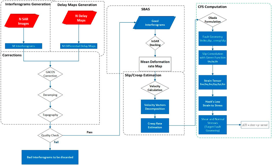
FIGURE 2. Flowchart of the processing technique employed in the study.
3 Results
Figures 3, 4 show a map of the mean LOS velocities in the study area. The estimated velocities of both the ascending and descending tracks range from −20 mm/yr to + 20 mm/yr, with a maximum rate of approximately 20 mm/yr on the descending track in the Khisor Range and southeast of the KBF. Such large displacements in the LOS direction can be caused by several factors, including 1) the choice of reference point, which is relative to the measurement of InSAR observations; 2) topography-related error due to the mountainous region; 3) unwrapping errors; and 4) cumulative loop closure, which shortens the interferogram interval, which can result in signal uplifting due to the presence of phase biases. We estimate each error’s contribution and subtract it from the mean LOS velocities field to separate the signal from the errors. Collectively, noise levels on the KBF are relatively low in the range of −2.5 mm/yr to 2.5 mm/yr (see Figures 3, 4). Figure 5 depicts the corrected final mean velocity maps in the LOS direction for both ascending and descending tracks. These maps are georeferenced to the global coordinate system. The STD in the velocity field (Figures 5C, D) is estimated from the cumulative displacement employing the percentile bootstrap method (Efron and Tibshirani, 1986). The lower STD shows the best estimate of the displacement rate. Figure 6 shows the STD of the unwrapping phase in the spatial domain before and after the GACOS correction for each interferogram. Figure 6 represents the overall effect of the GACOS correction on the unwrapped interferograms. However, 384 out of 570 and 241 out of 360 interferograms were corrected after implementing the GACOS correction in the ascending and descending tracks, respectively. The GACOS correction improved the STD of interferograms on average by decreasing the STD from 3.18 cm to 2.68 and 2.91 cm to 2.49 for the ascending and descending tracks, respectively. Similarly, the STD decreased from 2.87 to 2.34 cm and 2.61 to 2.03 cm on median after the GACOS correction. The worsened STD interferograms after the GACOS correction may be related to the low accuracy of the GACOS turbulence data (Wang et al., 2019). The worst interferograms from the ascending track (Figure 6A) and descending track (Figure 6B) were removed before the estimation of the rate map. After removing atmospheric noise, the residual noise in the velocity measurements is significantly reduced. Finally, the velocity field obtained from both ascending and descending tracks was decomposed to components by selecting only those pixels that were available in both rate maps. Assuming a fixed strike of 165°, the LOS velocity is decomposed to horizontal and vertical components using equation 2. Figure 7 illustrates these components. The steep gradient of the LOS velocity across the Kalabagh Fault on both tracks is the primary feature observed in Figure 5. This gradient has a similar sign on both tracks, indicating right-lateral motion. The gradient reaches approximately 10 mm/year along the LOS, as illustrated in Figures 2–5.
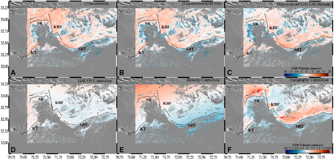
FIGURE 3. Cumulative effect of the corrections on (A) uncorrected LOS velocity deduced from Sentinel-1A InSAR data from the ascending track T: 173, (B) atmospheric corrected LOS velocity, and (D) GACOS correction. (C) Impact of the application of (E) deramp correction applied to (B); the resultant is named (uncorrected–GACOS–deramp). (F) Topography correction; the resultant is shown in Figure 5. Abbreviations of prominent faults and ranges shown in the map are SRT, Salt Range Thrust; KBF, Kalabagh Fault; SR, Surghar Ranges; and KT, Khisor Thrust.
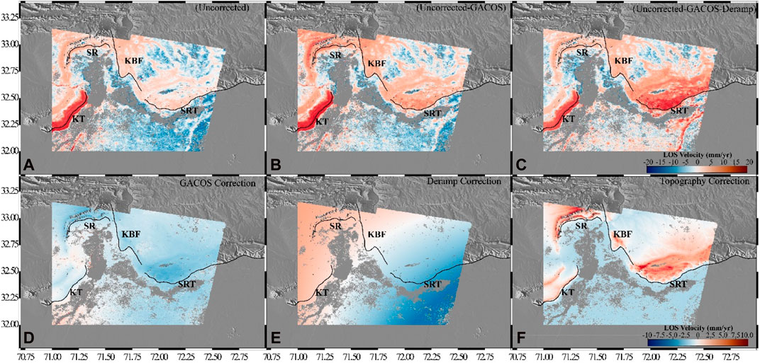
FIGURE 4. Cumulative effect of the corrections on (A) uncorrected LOS velocity deduced from Sentinel 1-A InSAR data from the descending track T:005, (B) atmospheric corrected LOS velocity, and (D) GACOS correction. (C) Impact of the application of (E) deramp correction applied to (B); the resultant is named (uncorrected–GACOS–deramp). (F) Topography correction; the resultant is shown in Figure 5. Abbreviations of prominent faults and ranges shown in the map are SRT: Salt Range Thrust, KBF: Kalabagh Fault, SR: Surghar Ranges, and KT: Khisor Thrust.
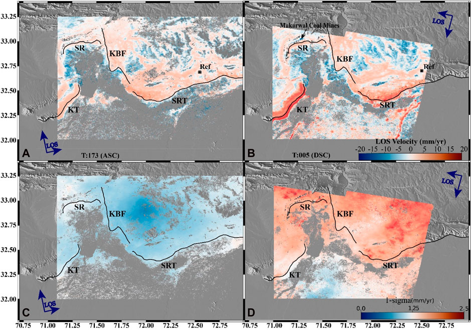
FIGURE 5. (A, B) Mean LOS velocity map relative to the reference point (Ref) computed from the ascending track (T: 173) and descending track (T: 005), respectively. (C, D) The 1-sigma error estimation in the rate map computed for ascending and descending tracks, respectively. After computing the rate map, it is filtered and corrected by GACOS, de-ramping, and topography. The motion toward the satellite is indicated by warm colors, and vice versa. Black lines represent the prominent faults in the study area. Abbreviations of prominent faults and ranges shown in the map are SRT: Salt Range Thrust, KBF: Kalabagh Fault, SR: Surghar Ranges, and KT: Khisor Thrust.
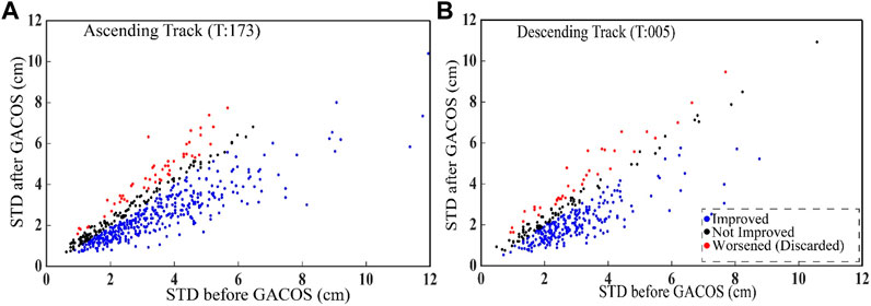
FIGURE 6. Standard deviation (STD) of the unwrapped phases in 570 ascending (A) and 360 descending (B) interferograms are correlated before and after the GACOS correction. Blue, black, and red dots represent the improved, not improved, and worsened interferograms, respectively.
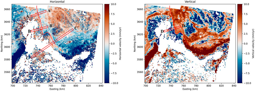
FIGURE 7. Decomposed horizontal and up/vertical velocity components after topography correction application. Red profiles across the fault are taken to measure the creep rate. Lat/Long in the map are converted to Easting Northing using datum WGS84.
Figure 8 shows cross-sections across the Kalabagh Fault, depicting the heterogeneous creeping along the fault’s strike. To avoid biases related to the topographic error, profiles are chosen at locations where the topography is almost identical on both sides of the fault. We plot a set of two 25 km-long AA/(on the northern segment of the KBF) and BB/(on the central segment of the KBF) and one 80 km-long CC/(on the southern segment of the KBF), cross-cutting the fault, as presented in Figure 8. Similarly, we plot the 25 km-long cross-section on the central section of Figure 8. Supplementary Figure S2 shows the profiles at the same fault segments without applying the topography correction. Each profile was kept consistently 2.5 km broad. The northern section of the KBF displays a significantly more pronounced horizontal velocity field discontinuity than the central section, which exhibits a higher fault-up velocity discontinuity. These observations are consistent with earlier InSAR and geological studies conducted by Chen and Khan (2010), McDougall and Hussain (1991), and McDougall and Khan (1990).
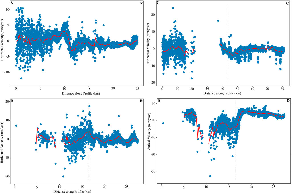
FIGURE 8. Pairs of horizontal and vertical components of velocity decomposed after applying topography correction for each profile (AA/, BB/, CC/, and DD/) are plotted and labeled in this figure. The dotted vertical line in each figure shows the location of the fault. Velocity components for each profile are shown on the ordinate, and the abscissa shows the distance along the profile as labeled. The blue dots depict velocity components at each pixel, whereas the red line shows the average velocity.
In order to analyze the creeping pattern along different segments of the fault, the LOS velocity components were inverted. This inversion enables us to quantify the creeping rate in the fault’s shallow region. We optimize the creep model parameters by considering a wide range of values for slip rates (ranging from 0 to 20 mm/yr), creep rates (ranging from 0 to 20 mm/yr), locking depths (ranging from 0 to 10 km), creep depths (ranging from 0 to 6 km), offset (ranging from −10–10 mm/yr), and offset from the fault (−20–20 km). These ranges were adopted based on previous studies conducted by Chen and Khan (2010), McDougall and Hussain (1991), and McDougall and Khan (1990). The observed signal may not always be perfectly aligned with the fault trace. In these cases, the offset to the location of the fault trace could be useful in order to get an accurate estimation of the creep rate and other parameters. The model parameters and their uncertainties are estimated through a Markov chain Monte Carlo approach. We use 1e6 iterations to define the posterior probability of the model using higher ranges of the model parameters. The maximum likelihood function by minimizing the weighted misfits is calculated between observations and models to rank the solutions. The first 20% of solutions are excluded as burn-in, whereas the remaining solutions are used to define the maximum a posteriori solution. The same approach was applied in previous studies on the estimation of creep or slip rates (Toda et al., 1998; Fattahi and Amelung, 2016). The velocity data on both sides of the fault were fitted with the best-fit 50 inversion models, as illustrated in Figure 9. We were unable to resolve the discontinuity over the KBF for the horizontal component of profile BB/ because of negligible components of these directional creep components. However, we adopted the (Barnhart, 2017; Okada, 1992) forward model to fit the vertical displacement. This study is intended to assess the general mechanics of the KBF, including the variation of creep rate along the fault, locking depth, and creep depth. The horizontal velocity step in profile AA′ is the most noticeable, and it has the largest creep rate (4.8 ± 1.6 mm/year) within error bars. In contrast, profile CC′ consistently displays a lower creep rate than profile AA′. The models for profile BB′ did not show any substantial horizontal creep, but they predicted a vertical creep rate of approximately 10 mm/year (profile DD′). All investigated profiles on the fault have shown varying creep patterns on all three sections of the KBF. However, the results have shown good consistency with earlier studies carried out by Chen and Khan (2010) and suggest that the creeping occurs at depths ranging from 0.5 to 6 km (as shown in Figure 9). Our model did not indicate any significant slip rate along the Kalabagh Fault, which is in agreement with the region’s overall tectonics as the viscous decollement is present over Kohat–Potwar fold and thrust fault (Smith et al., 1994; Jaswal et al., 1997; Satyabala et al., 2012; Javed et al., 2022). Another noteworthy aspect of the vertical velocity field during the study period of 2015–2022 is the subsidence pattern, as shown in Figure 7. However, the maximum displacements in the horizontal component along Khisor Thrust and Salt Range Thrust (SRT) are not associated with the tectonics. This arises due to resolving the horizontal components to the geometry of the KBF. Additionally, we observed an asymmetrical pattern of horizontal and vertical velocities across the KBF. This could be due to the variation of fault dip with depth and heterogeneities of the elastic crust (Fialko et al., 2002; Fialko, 2006; Javed, 2017). Asymmetric velocity patterns have also been observed in other major active strike–slip faults around the world, including the San Andreas Fault (SAF) in the United States (Fialko et al., 2002; Fialko, 2006) and the Idrija Fault System in Italy (Javed, 2017). The modeling of asymmetric patterns, on the other hand, is beyond the scope of this work.
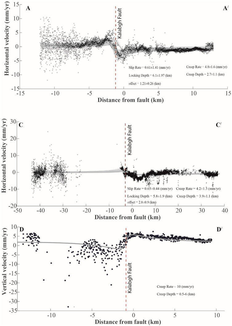
FIGURE 9. Southwest–northeast profiles of the decomposed velocity components against all three profiles (AA/, CC/, and DD/) along with the modeled best-fit solutions (i.e., gray lines) with locking and creep depths and individual creep and slip rates. The 0 km abscissa represents the location of the Kalabagh Fault adapted from the work of Chen and Khan (2009), whereas the red dotted line illustrates the position of the KBF from the inversion.
Finally, Coulomb 3.4 (Lin and Stein, 2004) was applied for computation of Coulomb failure stress changes (ΔCFS) to estimate the effect of creeping on local strike–slip and gentle dip (∼300) thrust faults. The strike of these other faults is taken similar to the KBF (i.e., strike ∼165), whereas the surface strike of the thrust geometry is adopted using rupture of local thrust faults (i.e., strike ∼ 250). Considering the creeping of the last 07 years, ΔCFS is computed more than 0.025 bar at 2.5 km and 5 km depths (see Figure 10). ΔCFS estimates positive on the northern and southeast regions of the KBF (see Figures 10C, D). However, the region of positive ΔCFS is limited to two small lobes on the right side of the KBF (Figures 10A, B).
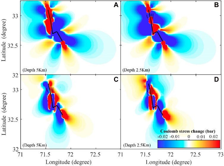
FIGURE 10. ΔCFS computed for target fault geometry (A, B) dextral strike–slip fault and (C, D) thrust fault at different depths as mentioned in the diagram.
4 Discussion
A previous InSAR study on the interseismic deformation in the Kohat–Potwar region relies on a single pair of descending SAR images of ERS-1/ERS-2 across the Kalabagh Fault (Chen and Khan, 2010). In the context of InSAR processing, strain variations along the strike are often disregarded. However, this study demonstrates the potential for detecting such variations along faults using the extensive radar data archive provided by the Sentinel-1A satellite and applied an optimized processing approach that accounts for the reduction of atmospheric noise, similar to the Main Recent Fault in SW Iran (Watson et al., 2022). Despite this progress, limitations in our modeling persist, particularly regarding the simplified geometry and homogenous Earth crust.
Several studies have been conducted to explore the development of the KBF system and the northwestern Himalayan frontal thrust system’s progression over time (Yeats et al., 1984; Yeats and Hussain, 1987; McDougall and Khan, 1990; McDougall and Hussain, 1991; Smith et al., 1994; Bender and Raza, 1995; Khan and Glenn, 2006). The existence of salt has complicated the geometry and structural pattern of the frontal thrust system (Butler, 1987). The structural arrangement of the basement rock is the main factor influencing the Kalabagh Fault Zone’s development (McDougall and Khan, 1990). As suggested by numerous studies, the thrusting propagates forward on brittle detachment layers over the evaporitic decollement and brittle layers (Cotton and Koyi, 2000; Costa and Vendeville, 2002; Schreurs et al., 2002). However, a prior analysis of InSAR data demonstrates that the Chisal Algad stream experiences a strike–slip displacement rate of 6.2 mm/yr (Chen and Khan, 2010). In the last two Ma, McDougall and Khan (1990) calculated that a dislocation of approximately 7–10 mm/a has occurred near the Chisel Algad River, and a slow creeping of about ∼3.7 mm/a also persists along the Nammal Ridge (Chen and Khan, 2010). The findings of Chen and Khan (2009) indicate that the thrusting process has not always propagated consistently on a viscous décollement in the relation of the SRT and the Potwar Plateau. The SRT wedge, on the other hand, is creeping on a thick salt décollement. Based on their findings, the researchers concluded that current internal deformation outweighs the frontal deformation. Additionally, the outcomes of geomorphic and tectonic investigations support the various deformation patterns (Chen and Khan, 2009; Chen and Khan, 2010; Abbas et al., 2022). For instance, the western portion of the Salt Range is rising approximately 10 mm/yr (Abir et al., 2015). Additionally, Abbas et al. (2022) demonstrated the compression at the KBF’s central section. Our creeping measurement findings (i.e., 4.8 ± 1.6 mm/yr on horizontal velocity) are consistent with the work of Chen and Khan (2009) and support the idea that the northern region of the KBF is currently undergoing internal deformation. The absence of an up-dip component of the creep rate in that section supports the claim of lesser southward thrusting propagation by the Kohat–Surghar thrust wedge due to the more resistant nature of brittle detachment. Based on our InSAR findings, the center portion of the KBF has shown 10 mm/yr vertical creeping, confirming previous research’s observations of uplift (McDougall and Khan, 1990; McDougall and Hussain, 1991; Abbas et al., 2022). In addition to this, the KBF also showed the velocity-weakening region below 4 km depth on both the northern and southern sections of the fault. The occurrence of earthquakes, as reported by Abbas et al. (2022), could be the result of partial creeping at depth. However, estimation of the slip rate and looking depth is poorly constrained. In comparison to the center and northern sections of the KBF, the southern section of the KBF demonstrates a relatively lower creep rate. The predicted horizontally creeping rate of ∼4.2 ± 1.3 mm/yr is in good accordance with the earlier observation for this section (Chen and Khan, 2010). Several earlier studies concluded that the Potwar–Kohat plateau is accommodating 5–10 mm/yr deformation, but these estimations are based on geological studies, sparse GPS estimation, and limited ERS-InSAR data coverage (Wells, 1984; Yeats et al., 1984; Yeats and Hussain, 1987; McDougall and Khan, 1990; McDougall and Hussain, 1991). A recent study by Abass et al. (2022) showed the shallow duplex structure of Kohat accommodating 5 mm/yr. Similarly, Jouanne et al. (2020) used modeling of interseismic coupling of MHT beneath Northern Pakistan and illustrated that the Potwar Plateau is creeping at a rate of approximately 6 mm/yr, which is approximately 20% of the total deformation rate (i.e., 3 cm/yr) between the Indian and Eurasian plates. Our estimates also show that the creeping rate along the Kalabagh Fault is approximately 5 mm/yr, so creeping is the dominant phenomenon beneath the Kohat–Potwar plateau. Last, the asymmetrical distribution of horizontal and vertical velocities over the KBF is connected to the lateral variation in rigidity caused by the presence of a significant salt layer to the east of the KBF and complex fault geometry at depth. The impact of various parameters is highlighted by several authors in their studies (Efron and Tibshirani, 1986; Le Pichon et al., 2005; Lindsey and Fialko, 2013).
Various models have been utilized in the past to comprehend the interaction between the Indian and Eurasian plates. The crustal thickening and shortening are accounted for by the thin viscous model. On the other hand, crustal shortening taking place along large-scale strike–slip boundaries is addressed by extrusion tectonics models (Molnar and Tapponnier, 1977; England and Houseman, 1989; Harrison et al., 1992; Houseman and England, 1993). However, the precise kinematics and geometry of extrusions are not yet fully understood, as many structures, such as transform faults that facilitate the extrusions, are not identified or accurately mapped. Structural geometry disparities are frequent in the Himalayan orogeny, as noted by Chen and Khan (2010), and these variations significantly impact the deformation pattern, outcrop generations and movements, and sedimentary history of the orogeny, as discussed by Yin and Harrison (2000).
Finally, the interaction between the KBF and nearby local strike–slip and thrust faults are evaluated using the Coulomb stress changes. In the past, numerous studies demonstrated that ΔCFS >0.01 MPa is enough to trigger seismicity (Toda et al., 1998). To the east of the KBF, the decollement thrust–fold assemblages are the prominent features of the Potwar Plateau. However, the Indian Plate slips aseismically beneath the Kohat–Potwar thrust and fold belt (Satyabala et al., 2012), so large earthquakes are unlikely in this region due to viscous decollement (Satyabala et al., 2012). However, this region is characterized by a partial stick–slip phenomenon occurring on one or more locked portions of fault on the ramp for longer temporal gaps that are connected to the decollement. The increase in stress loading on adjacent fault segments (i.e., northern and southeast of the KBF) can have serious seismic implication.
5 Conclusion
Sentinel-1A ascending and descending data for the period of 2015–2022 are used to compute the rate map of the KBF, one of the distinctive features of the Indian and Eurasian plate collision. Our inversion showed a variation of creep rates at different segments of the fault. Horizontally and vertically decomposed components of velocity at three different cross profiles of the KBF zone are presented in this study. The fault creeping rates corresponding to the horizontal component at the northern segment and southern end of the fault showed creep rates of ∼ 4.8 ± 1.6 and ∼4.2 ± 1.3 mm/year, respectively, whereas the central section of the fault showed negligible horizontal component of velocity but a vertical component of ∼10 mm/year. The up-dip creep rate illustrates the rapid vertical uplift at the central fault segment of the KBF and is in good accordance with the thrusting and folding. Moreover, our model did not rule out an interseismic slip rate at depth, which could be linked to earthquakes in the past. Our findings of the heterogenous creep rate on the KBF will assist the understanding of the mechanics of Indian–Eurasian collision. This study will enable us to better address the seismic hazard assessment in the region.
Data availability statement
The original contributions presented in the study are included in the article/Supplementary Material; further inquiries can be directed to the corresponding author.
Author contributions
All authors listed made a substantial, direct, and intellectual contribution to the work and approved it for publication.
Funding
The authors thank and express their gratitude to the Researchers Supporting Project (RSP2023R249), King Saud University, Riyadh, Saudi Arabia, for funding this research article.
Acknowledgments
The authors thank the center for Earthquake Studies (CES), National Centre for Physics, Islamabad and Advance Computational Reactor Engineering (ACRE) Lab, PIEAS, Islamabad for providing the computational facility to accomplish the research. They thank the ESA for making the Sentinel-1A data available in public domain for research purposes. FJ is grateful to the ICTP Associates Program (2020–2025) for providing support. The authors thank and express their gratitude to the Researchers Supporting Project (RSP2023R249), King Saud University, Riyadh, Saudi Arabia, for funding this research article.
Conflict of interest
The authors declare that the research was conducted in the absence of any commercial or financial relationships that could be construed as a potential conflict of interest.
Publisher’s note
All claims expressed in this article are solely those of the authors and do not necessarily represent those of their affiliated organizations, or those of the publisher, the editors, and the reviewers. Any product that may be evaluated in this article, or claim that may be made by its manufacturer, is not guaranteed or endorsed by the publisher.
Supplementary Material
The Supplementary Material for this article can be found online at: https://www.frontiersin.org/articles/10.3389/feart.2023.1231408/full#supplementary-material
References
Abbas, W., Ali, S., and Reicherter, K. (2022). Seismicity and landform development of the dextral Kalabagh Fault Zone, Pakistan: Implications from morphotectonics and paleoseismology. Tectonophysics 822, 229182. doi:10.1016/j.tecto.2021.229182
Abir, I. A., Khan, S. D., Ghulam, A., Tariq, S., and Shah, M. T. (2015). Active tectonics of Western Potwar Plateau--Salt Range, northern Pakistan from InSAR observations and seismic imaging. Remote Sens. Environ. 168, 265–275. doi:10.1016/j.rse.2015.07.011
Baker, D. M., Lillie, R. J., Yeats, R. S., Johnson, G. D., Yousuf, M., and Zamin, A. S. H. (1988). Development of the himalayan frontal thrust zone: Salt range, Pakistan. Geology 16 (1), 3–7. doi:10.1130/0091-7613(1988)016<0003:dothft>2.3.co;2
Barnhart, W. D. (2017). Fault creep rates of the Chaman fault (Afghanistan and Pakistan) inferred from InSAR. J. Geophys. Res. Solid Earth 122 (1), 372–386. doi:10.1002/2016jb013656
Beck, R. A., Burbank, D. W., Sercombe, W. J., Riley, G. W., Barndt, J. K., Berry, J. R., et al. (1995). Stratigraphic evidence for an early collision between northwest India and Asia. Nature 373 (6509), 55–58. doi:10.1038/373055a0
Bender, F., and Raza, H. A. (1995). Geology of Pakistan. Berlin, Germany: Gebruder Borntraeger, 11–63.
Berardino, P., Casu, F., Fornaro, G., Lanari, R., Manunta, M., Manzo, M., et al. (2003). Small baseline DIFSAR techniques for Earth surface deformation analysis. Third Int. Workshop ERS SAR Interferom. ‘FRINCE03 6. doi:10.3390/s19224857
Biggs, J., and Wright, T. J. (2020). How satellite InSAR has grown from opportunistic science to routine monitoring over the last decade. Nat. Commun. 11 (1), 3863–3864. doi:10.1038/s41467-020-17587-6
Blisniuk, P. M., Sonder, L. J., and Lillie, R. J. (1998). Foreland normal fault control on northwest Himalayan thrust front development. Tectonics 17 (5), 766–779. doi:10.1029/98tc01870
Borghi, A., Aoudia, A., Javed, F., and Barzaghi, R. I. C. C. A. R. D. O. (2016). Precursory slow-slip loaded the 2009 L'Aquila earthquake sequence. Geophys. J. Int. 205 (2), 776–784. doi:10.1093/gji/ggw046
Bürgmann, R., Rosen, P. A., and Fielding, E. J. (2000). Synthetic aperture radar interferometry to measure Earth’s surface topography and its deformation. Annu. Rev. Earth Planet. Sci. 28 (1), 169–209. doi:10.1146/annurev.earth.28.1.169
Butler, R. W. H. (1987). Thrust sequences. J. Geol. Soc. 144 (4), 619–634. doi:10.1144/gsjgs.144.4.0619
Castellazzi, P., Arroyo-Dom\’\inguez, N., Martel, R., Calderhead, A. I., Normand, J. C. L., Gárfias, J., et al. (2016). Land subsidence in major cities of Central Mexico: Interpreting InSAR-derived land subsidence mapping with hydrogeological data. Int. J. Appl. Earth Observation Geoinformation 47, 102–111. doi:10.1016/j.jag.2015.12.002
Cavalié, O., Lasserre, C., Doin, M.-P., Peltzer, G., Sun, J., Xu, X., et al. (2008). Measurement of interseismic strain across the Haiyuan fault (Gansu, China), by InSAR. Earth Planet. Sci. Lett. 275 (3–4), 246–257. doi:10.1016/j.epsl.2008.07.057
Chen, C. W., and Zebker, H. A. (2002). Phase unwrapping for large SAR interferograms: Statistical segmentation and generalized network models. IEEE Trans. Geoscience Remote Sens. 40 (8), 1709–1719. doi:10.1109/tgrs.2002.802453
Chen, L., and Khan, S. D. (2009). Geomorphometric features and tectonic activities in sub-Himalayan thrust belt, Pakistan, from satellite data. Comput. \& Geosci. 35 (10), 2011–2019. doi:10.1016/j.cageo.2008.11.011
Chen, L., and Khan, S. D. (2010). InSAR observation of the strike-slip faults in the northwest Himalayan frontal thrust system. Geosphere 6 (5), 731–736. doi:10.1130/ges00518.1
Chen, T., Liu-Zeng, J., Shao, Y., Zhang, P., Oskin, M. E., Lei, Q., et al. (2018). Geomorphic offsets along the creeping Laohu Shan section of the Haiyuan fault, northern Tibetan Plateau. Geosphere 14 (3), 1165–1186. doi:10.1130/ges01561.1
Costa, E., and Vendeville, B. C. (2002). Experimental insights on the geometry and kinematics of fold-and-thrust belts above weak, viscous evaporitic décollement. J. Struct. Geol. 24 (11), 1729–1739. doi:10.1016/s0191-8141(01)00169-9
Cotton, J. T., and Koyi, H. A. (2000). Modeling of thrust fronts above ductile and frictional detachments: Application to structures in the Salt Range and Potwar Plateau, Pakistan. Geol. Soc. Am. Bull. 112 (3), 351–363. doi:10.1130/0016-7606(2000)112<351:motfad>2.0.co;2
Efron, B., and Tibshirani, R. J. S. s. (1986). Bootstrap methods for standard errors, confidence intervals, and other measures of statistical accuracy. Stat. Sci. 1, 54–75. doi:10.1214/ss/1177013816
England, P., and Houseman, G. (1989). Extension during continental convergence, with application to the Tibetan Plateau. J. Geophys. Res. Solid Earth 94 (B12), 17561–17579. doi:10.1029/jb094ib12p17561
Fattahi, H., and Amelung, F. (2016). InSAR observations of strain accumulation and fault creep along the Chaman Fault system, Pakistan and Afghanistan. Geophys. Res. Lett. 43 (16), 8399–8406. doi:10.1002/2016gl070121
Ferretti, A., Fumagalli, A., Novali, F., Prati, C., Rocca, F., and Rucci, A. (2011). A new algorithm for processing interferometric data-stacks: SqueeSAR. IEEE Trans. Geoscience Remote Sens. 49 (9), 3460–3470. doi:10.1109/tgrs.2011.2124465
Fialko, Y. (2006). Interseismic strain accumulation and the earthquake potential on the southern San Andreas fault system. Nature 441 (7096), 968–971. doi:10.1038/nature04797
Fialko, Y., Sandwell, D., Agnew, D., Simons, M., Shearer, P., and Minster, B. (2002). Deformation on nearby faults induced by the 1999 Hector Mine earthquake. Science 297 (5588), 1858–1862. doi:10.1126/science.1074671
Ghorbani, Z., Khosravi, A., Maghsoudi, Y., Mojtahedi, F. F., Javadnia, E., and Nazari, A. (2022). Use of InSAR data for measuring land subsidence induced by groundwater withdrawal and climate change in Ardabil Plain, Iran. Iran 12 (1), 13998–14022. doi:10.1038/s41598-022-17438-y
Harrison, T. M., Copeland, P., Kidd, W. S. F., and Yin, A. N. (1992). Raising tibet. Science 255 (5052), 1663–1670. doi:10.1126/science.255.5052.1663
Hooper, A. (2008). A multi-temporal InSAR method incorporating both persistent scatterer and small baseline approaches. Geophys. Res. Lett. 35 (16), L16302. doi:10.1029/2008gl034654
Hooper, A., and Zebker, H. A. J. J. A. (2007). Phase unwrapping in three dimensions with application to InSAR time series. J. Opt. Soc. Am. A 24 (9), 2737–2747. doi:10.1364/josaa.24.002737
Hough, S. E., and Bilham, R. (2018). Poroelastic stress changes associated with primary oil production in the Los Angeles Basin, California. Lead. Edge 37 (2), 108–116. doi:10.1190/tle37020108.1
Houseman, G., and England, P. (1993). Crustal thickening versus lateral expulsion in the Indian-Asian continental collision. J. Geophys. Res. Solid Earth 98 (B7), 12233–12249. doi:10.1029/93jb00443
Houseman, G., and England, P. (1986). Finite strain calculations of continental deformation: 1. Method and general results for convergent zones. J. Geophys. Res. Solid Earth 91 (B3), 3651–3663. doi:10.1029/jb091ib03p03651
Hsieh, C.-S., Shih, T.-Y., Hu, J.-C., Tung, H., Huang, M.-H., and Angelier, J. (2011). Using differential SAR interferometry to map land subsidence: A case study in the pingtung plain of SW taiwan. Nat. Hazards 58 (3), 1311–1332. doi:10.1007/s11069-011-9734-7
Hussain, E., Hooper, A., Wright, T. J., Walters, R. J., and Bekaert, D. P. S. (2016). Interseismic strain accumulation across the central North Anatolian Fault from iteratively unwrapped InSAR measurements. J. Geophys. Res. Solid Earth 121 (12), 9000–9019. doi:10.1002/2016jb013108
Jaswal, T. M., Lillie, R. J., and Lawrence, R. D. (1997). Structure and evolution of the northern Potwar deformed zone, Pakistan. AAPG Bull. 81 (2), 308–328. doi:10.1306/522b431b-1727-11d7-8645000102c1865d
Javed, F. (2017). Earthquake transients and mechanics of active deformation: Case studies from Pakistan and Italy. United States: Università degli Studi di Trieste. doi:10.1029/gm037p0297
Javed, M. T., Barbot, S., Javed, F., Ali, A., and Braitenberg, C. J. G. R. L. (2022). Coseismic folding during ramp failure at the front of the Sulaiman fold-and-thrust belt. Geophys. Res. Lett. 2022, e2022GL099953. doi:10.1029/2022gl099953
Johanson, I. A., and Bürgmann, R. (2005). Creep and quakes on the northern transition zone of the San Andreas fault from GPS and InSAR data. Geophys. Res. Lett. 32 (14). doi:10.1029/2005gl023150
Jolivet, R., Lasserre, C., Doin, M.-P., Guillaso, S., Peltzer, G., Dailu, R., et al. (2012). Shallow creep on the Haiyuan fault (Gansu, China) revealed by SAR interferometry. J. Geophys. Res. Solid Earth 117 (B6). doi:10.1029/2011jb008732
Jolivet, R., Lasserre, C., Doin, M.-P., Peltzer, G., Avouac, J.-P., Sun, J., et al. (2013). Spatio-temporal evolution of aseismic slip along the Haiyuan fault, China: Implications for fault frictional properties. Earth Planet. Sci. Lett. 377, 23–33. doi:10.1016/j.epsl.2013.07.020
Khan, S. D., and Glenn, N. F. (2006). New strike-slip faults and litho-units mapped in Chitral (N. Pakistan) using field and ASTER data yield regionally significant results. Int. J. Remote Sens. 27 (20), 4495–4512. doi:10.1080/01431160600721830
Le Pichon, A., Herry, P., Mialle, P., Vergoz, J., Brachet, N., Garcés, M., et al. (2005). Infrasound associated with 2004--2005 large Sumatra earthquakes and tsunami. Geophys. Res. Lett., 32(19). doi:10.1029/2005gl023893
Lee, J.-C., Angelier, J., Chu, H.-T., Hu, J.-C., Jeng, F.-S., and Rau, R.-J. (2003). Active fault creep variations at Chihshang, Taiwan, revealed by creep meter monitoring, 1998--2001. J. Geophys. Res. Solid Earth 108 (B11), 2528. doi:10.1029/2003jb002394
Lin, J., and Stein, R. S. (2004). Stress triggering in thrust and subduction earthquakes and stress interaction between the southern San Andreas and nearby thrust and strike-slip faults. J. Geophys. Res. Solid Earth 109 (B2). doi:10.1029/2003jb002607
Lindsey, E. O., and Fialko, Y. (2013). Geodetic slip rates in the southern San Andreas Fault system: Effects of elastic heterogeneity and fault geometry. J. Geophys. Res. Solid Earth 118 (2), 689–697. doi:10.1029/2012jb009358
McDougall, J. W., and Hussain, A. (1991). Fold and thrust propagation in the Western Himalaya based on a balanced cross section of the Surghar Range and Kohat Plateau, Pakistan. AAPG Bull. 75 (3), 463–478. doi:10.1306/0c9b280d-1710-11d7-8645000102c1865d
McDougall, J. W., and Khan, S. H. (1990). Strike-slip faulting in a Foreland Fold-thrust belt: The Kalabagh Fault and western salt range, Pakistan. Tectonics 9 (5), 1061–1075. doi:10.1029/tc009i005p01061
Molnar, P., and Tapponnier, P. (1977). Relation of the tectonics of eastern China to the India-Eurasia collision: Application of slip-line field theory to large-scale continental tectonics. Geology, 5(4), 212–216. doi:10.1130/0091-7613(1977)5<212:rottoe>2.0.co;22 `
Morishita, Y., Lazecky, M., Wright, T. J., Weiss, J. R., Elliott, J. R., and Hooper, A. (2020). LiCSBAS: An open-source InSAR time series analysis package integrated with the LiCSAR automated Sentinel-1 InSAR processor. Remote Sens. 12 (3), 424. doi:10.3390/rs12030424
Morishita, Y. (2021). Nationwide urban ground deformation monitoring in Japan using Sentinel-1 LiCSAR products and LiCSBAS. Prog. Earth Planet. Sci. 8 (1), 6–23. doi:10.1186/s40645-020-00402-7
Mousavi, Z., Pathier, E., Walker, R. T., Walpersdorf, A., Tavakoli, F., Nankali, H., et al. (2015). Interseismic deformation of the Shahroud fault system (NE Iran) from space-borne radar interferometry measurements. Geophys. Res. Lett. 42 (14), 5753–5761. doi:10.1002/2015gl064440
Ng, A. H.-M., Wang, H., Dai, Y., Pagli, C., Chen, W., Ge, L., et al. (2018). InSAR reveals land deformation at Guangzhou and Foshan, China between 2011 and 2017 with COSMO-SkyMed data. Remote Sens. 10 (6), 813. doi:10.3390/rs10060813
Okada, Y. (1992). Internal deformation due to shear and tensile faults in a half-space. Bull. Seismol. Soc. Am. 82 (2), 1018–1040. doi:10.1785/bssa0820021018
Peltzer, G., Crampé, F., Hensley, S., and Rosen, P. (2001). Transient strain accumulation and fault interaction in the Eastern California shear zone. Geology 29 (11), 975–978. doi:10.1130/0091-7613(2001)029<0975:tsaafi>2.0.co;2
Pogue, K. R., Wardlaw, B. R., Harris, A. G., and Hussain, A. (1992). Paleozoic and mesozoic stratigraphy of the Peshawar Basin, Pakistan: Correlations and implications. Geol. Soc. Am. Bull. 104 (8), 915–927. doi:10.1130/0016-7606(1992)104<0915:pamsot>2.3.co;2
Pope, N., and Mooney, W. D. (2020). Coulomb stress models for the 2019 Ridgecrest, California earthquake sequence. Tectonophysics 791, 228555. doi:10.1016/j.tecto.2020.228555
Prati, C., Ferretti, A., and Perissin, D. (2010). Recent advances on surface ground deformation measurement by means of repeated space-borne SAR observations. J. Geodyn. 49 (3–4), 161–170. doi:10.1016/j.jog.2009.10.011
Pudsey, C. J. (1986). The northern suture, Pakistan: Margin of a cretaceous island arc. Geol. Mag. 123 (4), 405–423. doi:10.1017/s0016756800033501
Rosen, P., Werner, C., Fielding, E., Hensley, S., Buckley, S., and Vincent, P. (1998). Aseismic creep along the San Andreas Fault northwest of Parkfield, CA measured by radar interferometry. Geophys. Res. Lett. 25 (6), 825–828. doi:10.1029/98gl50495
Rosi, A., Tofani, V., Tanteri, L., Tacconi Stefanelli, C., Agostini, A., Catani, F., et al. (2018). The new landslide inventory of tuscany (Italy) updated with PS-InSAR: Geomorphological features and landslide distribution. Landslides 15 (1), 5–19. doi:10.1007/s10346-017-0861-4
Satyabala, S. P., Yang, Z., and Bilham, R. (2012). Stick--slip advance of the Kohat plateau in Pakistan. Nat. Geosci. 5 (2), 147–150. doi:10.1038/ngeo1373
Savage, J. C., and Lisowski, M. (1993). Inferred depth of creep on the Hayward fault, central California. J. Geophys. Res. Solid Earth 98 (B1), 787–793. doi:10.1029/92jb01871
Savage, J. C., and Prescott, W. H. (1978). Asthenosphere readjustment and the earthquake cycle. J. Geophys. Res. Solid Earth 83 (B7), 3369–3376. doi:10.1029/jb083ib07p03369
Schreurs, G., Hänni, R., and Vock, P. (2002). Analogue modelling of transfer zones in fold-and-thrust belts: A 4-D analysis. J. Virtual Explor. 7, 67–73. doi:10.3809/jvirtex.2002.00047
Segall, P. (2010). “Earthquake and volcano deformation,” in Earthquake and volcano deformation (United States: Princeton University Press). doi:10.1515/9781400833856.200
Smith, H. A., Chamberlain, C. P., and Zeitler, P. K. (1994). Timing and duration of Himalayan metamorphism within the Indian plate, northwest Himalaya, Pakistan. J. Geol. 102 (5), 493–508. doi:10.1086/629694
Titus, S. J., DeMets, C., and Tikoff, B. (2006). Thirty-five-year creep rates for the creeping segment of the San Andreas fault and the effects of the 2004 Parkfield earthquake: Constraints from alignment arrays, continuous global positioning system, and creepmeters. Bull. Seismol. Soc. Am. 96 (4B), S250–S268. doi:10.1785/0120050811
Toda, S., Stein, R. S., Reasenberg, P. A., Dieterich, J. H., and Yoshida, A. (1998). Stress transferred by the 1995M<sub>w</sub>= 6.9 Kobe, Japan, shock: Effect on aftershocks and future earthquake probabilities. J. Geophys. Res. Solid Earth 103 (B10), 24543–24565. doi:10.1029/98jb00765
Tong, X., Sandwell, D. T., and Smith-Konter, B. (2013). High-resolution interseismic velocity data along the san Andreas fault from GPS and InSAR. J. Geophys. Res. Solid Earth 118 (1), 369–389. doi:10.1029/2012jb009442
Walters, R. J., Elliott, J. R., Li, Z., and Parsons, B. (2013). Rapid strain accumulation on the Ashkabad fault (Turkmenistan) from atmosphere-corrected InSAR. J. Geophys. Res. Solid Earth 118 (7), 3674–3690. doi:10.1002/jgrb.50236
Wang, Q., Yu, W., Xu, B., and Wei, G. (2019). Assessing the use of GACOS products for SBAS-InSAR deformation monitoring: A case in southern California. Sensors 19, 3894. doi:10.3390/s19183894
Watson, A. R., Elliott, J. R., and Walters, R. J. (2022). Interseismic strain accumulation across the main Recent Fault, SW Iran, from sentinel-1 InSAR observations. J. Geophys. Res. Solid Earth 127 (2), e2021JB022674. doi:10.1002/essoar.10507719.1
Weiss, J. R., Walters, R. J., Morishita, Y., Wright, T. J., Lazecky, M., Wang, H., et al. (2020). High-resolution surface velocities and strain for Anatolia from Sentinel-1 InSAR and GNSS data. Geophys. Res. Lett., 47(17), e2020GL087376. doi:10.31223/osf.io/8xa7j
Wells, N. A. (1984). Marine and continental sedimentation in the early Cenozoic Kohat Basin and adjacent northwestern Indo-Pakistan. Michigan: University of Michigan. doi:10.1016/0025-3227(91)90061-8
Werner, C., Wegmuller, U., Strozzi, T., and Wiesmann, A. (2003). Interferometric point target analysis for deformation mapping IGARSS 2003 2003 IEEE international geoscience and Remote sensing symposium. Proc. (IEEE Cat. No. 03CH37477) 7, 4362–4364. doi:10.1109/igarss.2003.1295516
Wright, T. J., Parsons, B., England, P. C., and Fielding, E. J. (2004). InSAR observations of low slip rates on the major faults of Western Tibet. Science 305 (5681), 236–239. doi:10.1126/science.1096388
Xiong, X., Shan, B., Zhou, Y. M., Wei, S. J., Li, Y. D., Wang, R. J., et al. (2017). Coulomb stress transfer and accumulation on the Sagaing Fault, Myanmar, over the past 110 years and its implications for seismic hazard. Geophys. Res. Lett. 44 (10), 4781–4789. doi:10.1002/2017gl072770
Xu, Y.-S., Shen, S.-L., Ren, D.-J., and Wu, H.-N. (2016). Analysis of factors in land subsidence in shanghai: A view based on a strategic environmental assessment. Sustainability 8 (6), 573. doi:10.3390/su8060573
Yeats, R. S., and Hussain, A. (1987). Timing of structural events in the Himalayan foothills of northwestern Pakistan. Geol. Soc. Am. Bull. 99 (2), 161–176. doi:10.1130/0016-7606(1987)99<161:toseit>2.0.co;2
Yeats, R. S., Khan, S. H., and Akhtar, M. (1984). Late quaternary deformation of the salt range of Pakistan. Geol. Soc. Am. Bull. 95 (8), 958–966. doi:10.1130/0016-7606(1984)95<958:lqdots>2.0.co;2
Yin, A., and Harrison, T. M. (2000). Geologic evolution of the Himalayan-Tibetan orogen. Annu. Rev. Earth Planet. Sci. 28 (1), 211–280. doi:10.1146/annurev.earth.28.1.211
Yu, X., Hu, J., and Sun, Q. (2017). Estimating actual 2D ground deformations induced by underground activities with cross-heading InSAR measurements. J. Sensors 2017, 1–12. doi:10.1155/2017/3170506
Keywords: SAR interferometry, creeping, inversion, Coulomb stress, strike–slip fault
Citation: Zafar WA, Javed F, Ahmed R, Ehsan M, Abdelrahman K, Fnais MS and Qureshi MA (2023) Mechanics of the Kalabagh Fault, northwest Himalayan fold and thrust belt (convergence zone of India and Eurasia), using SAR interferometry and CFS. Front. Earth Sci. 11:1231408. doi: 10.3389/feart.2023.1231408
Received: 30 May 2023; Accepted: 17 July 2023;
Published: 02 August 2023.
Edited by:
Majid Khan, University of Science and Technology Beijing, ChinaReviewed by:
Yong Zheng, China University of Geosciences Wuhan, ChinaM. Younis Khan, University of Peshawar, Pakistan
Copyright © 2023 Zafar, Javed, Ahmed, Ehsan, Abdelrahman, Fnais and Qureshi. This is an open-access article distributed under the terms of the Creative Commons Attribution License (CC BY). The use, distribution or reproduction in other forums is permitted, provided the original author(s) and the copyright owner(s) are credited and that the original publication in this journal is cited, in accordance with accepted academic practice. No use, distribution or reproduction is permitted which does not comply with these terms.
*Correspondence: Muhsan Ehsan, bXVoc2FuZWhzYW45OEBob3RtYWlsLmNvbQ==