A rapid method for computing 3-D high-resolution vegetative canopy winds in weakly complex terrain

To determine near-surface winds within and above vegetation canopies for operational environmental applications, a wind model must run at high-resolution ($\mathcal{O}$(1–10 m)), in a few minutes, using limited input information, and requiring minimal computing resources (e.g., personal computers). Current research models simulate large domains at coarse resolution or small domains at fine scale, but canopy simulations can take days. Fast-modeling approaches are used to solve large complex wind fields, but they oversimplify the roughness elements’ distribution impact on momentum exchanges. To overcome these deficits, the fast-running wind model QUIC-URB (Quick Urban and Industrial Complex) was augmented with a high-resolution canopy wind solver. The wind model includes a non-local factor that describes how momentum propagates through the canopy and how sub-canopy jets appear under certain conditions. QUIC-URB was also coupled with the mesoscale WRF (Weather Research and Forecasting) model to downscale wind fields from a few kilometers to a meter. The new QUIC Canopy Model resolves 3-D wind fields over hundreds of millions of cells in less than 30 s per time step on a personal computer. It was compared to two canopy models for real quasi-homogeneous and heterogeneous canopies. An error analysis shows that the model was relatively accurate with a normalized root-mean-square error of about 0.2 m s⁻¹ in the quasi-homogeneous canopy, and a mean absolute error of 0.3 m s⁻¹. The new model is suitable for coupling with pollution dispersion, wildfire spread, and numerical weather prediction models over weakly complex terrain, defined here as a mildly undulating environment with gradual changes in elevation and a heterogeneous distribution of plants.

1 Introduction

Knowledge of the complex wind patterns ubiquitous in nature is essential to our understanding of many environmental applications. Wind provides energy to turbines (Porté-Agel et al., 2020), dissipates pollution (Amorim et al., 2013), transports seeds (Nathan et al., 2002), carries pests and pathogens in crops (Mahaffee et al., 2023), and drives wildfire propagation (Moody et al., 2022). Accurately forecasting the winds at relevant scales for human applications (meters to kilometers, every few minutes to days), at every location in a 3-D space, and in particular close to the ground surface, is needed to support the development and safety of communities at risk from natural catastrophes. Unfortunately, high-resolution wind forecasts are very costly in terms of computer resources. They are orders of magnitude more computationally expensive when individual buildings, forests, canyons, etc., are accounted for, and we are seemingly decades away from possessing the suitable technology to solve this issue without dramatically simplifying the problem. An exhaustive assessment of the numerical wind models’ grid resolution range recently achieved is available in Figure 4 and Section 4, in Stoll et al. (2020).

In the atmospheric boundary layer, three factors primarily define a wind field (e.g., Stull, 1988): the distribution of roughness elements including trees, buildings, and terrain elevation changes; the atmospheric stability, a measure of the influence of temperature gradients on the fluid motion; and the synoptic conditions, how the wind flows above the atmospheric boundary layer. The combination of these elements often gives rise to turbulence, which governs wind motion from planetary scales to dissipation scales, where the smallest eddies convert mechanical energy into thermal energy at the Kolmogorov scale (a few millimeters). In nature, urban or plant canopies can generate highly coherent turbulent structures that dominate turbulent fluxes (Brunet, 2020; Finnigan et al., 2020). Understanding these structures is key to modeling wind fields and particle dispersion because they govern how the wind momentum is absorbed and dissipated within and above a canopy. Indeed, observations and modeling show that the distribution of canopy elements is directly linked to the wind attenuation in dense environments (Nieto et al., 2019), and recirculations near ground-level or channeling between elements [e.g., streets in Neophytou et al. (2011), or forest edges in Hoffman et al. (2015)]. In this article, we restrict our scope to the impact of vegetative canopies on 3-D wind fields. Vegetation elements are assumed to be homogeneously distributed within small volumes of air close to the surface, so spatial averaging methods remain reliable at a few-meter resolution. As shown in Figure 1, denser regions of the forest tend to strongly reduce the wind speed. It is particularly true closer to the ground, but the canopy hardly affects the wind velocity above two or three times the effective tree height, in general (Brunet, 2020).

FIGURE 1

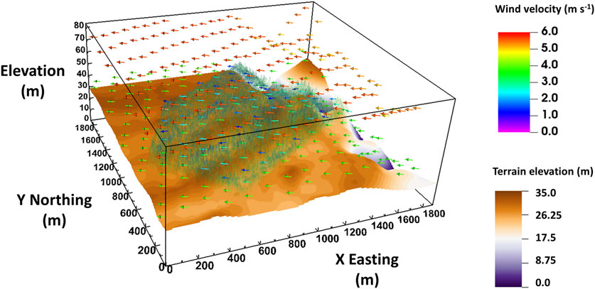
FIGURE 1. Wind velocity vector field at 10 and 50 m above ground level. Here, the QCM simulation domain covers the RxCADRE campaign L2F site. The terrain elevation scale starts at the lowest simulation domain altitude. As shown, the forest was heterogeneous, with dense patches on the southwest and northwest sides. Winds were stronger in clearings or outside of the forest. Average tree height was 12 m and the canopy did not impact the wind field above three times its height. At 50 m above ground level, the winds were more homogeneous and a function of the synoptic wind conditions rather than the terrain elements.

In order to forecast winds, the conservation equations for mass, momentum, and energy are solved using computational fluid dynamics (CFD) models that integrate environmental effects via boundary conditions and supplemental forcing terms. The accuracy of the predictions from these simulations depends on the simplifications made to the governing equations as well as the numerical implementation of the equations. Direct numerical simulations (DNS), the highest-fidelity method available, solve the flow equations down to the Kolmogorov scale (Moin and Mahesh, 1998). Large-eddy simulations (LES) solve the NSE for scales where the turbulence contains the most energy and apply parameterizations to the filtered quantities (Piomelli, 1999; Stoll et al., 2020). These techniques have contributed considerably to our understanding of how the wind flows in a complex environment, e.g., along slopes, within canopies, and on hillsides with vegetation (Bailey and Stoll, 2016; Ma et al., 2020; Sharma and García-Mayoral, 2020). Despite their achievements, DNS and LES remain highly time-consuming and require hours of computation on supercomputers to simulate domains of tens of meters. While Table 1 shows that simulations were run for highly idealized canopies, the authors have no knowledge of DNS results in realistic canopy conditions to date.

TABLE 1

TABLE 1. Comparative performance of the most commonly used numerical wind models for simulations with a vegetation canopy arranged from most accurate to simplest.

Less accurate but significantly faster, Reynolds-averaged Navier-Stokes (RANS) models compute statistically averaged quantities. After the averaging procedure, NSE non-linearity leads to a closure problem with more unknowns than equations, and a turbulent stress term arises (cf. Eq. 8). RANS models then differ in the number and type of equations used to model this additional term. Typically, vegetation influence is represented by adding a body force term in the RANS equations (Shaw, 1977; Macdonald, 2000; Segalini et al., 2016).

Numerical weather prediction (NWP) models rely on the RANS approach and observational data assimilation to produce mesoscale (10³–10⁵ m) wind forecasts and analysis. State-of-the-art NWP models, such as the Weather Research and Forecasting model (WRF, Skamarock et al., 2008), represent the effects of turbulence with a high level of sophistication. In most routine WRF simulations, the surface elements (e.g., canopy, streams, buildings, glaciers) are associated with broad land-use categories (LUC, Golzio et al., 2021). As expected, LUC fail to provide precise information for high spatial resolution simulations. In tools like WRF-SFIRE (a modeling system that combines WRF with a semi-empirical fire-spread model, Mandel et al., 2011; Mallia et al., 2020), the WRF LUC is replaced and canopy cover influence is instead resolved with a high level of detail using surface fuels in-situ measurements (Ottmar et al., 2016b) and a canopy sub-model based on Massman et al. (2017). Other recent approaches have also incorporated the variation of vegetation canopy elements and modeled canopy winds in WRF simulations (Arthur et al., 2019; Ma and Liu, 2019). Nonetheless, high-resolution NWP simulations over large domains presently require a large amount of computational resources.

Diagnostic wind models (DWMs) deliver high-resolution wind fields over large domains much faster than the aforementioned models (see Ratto et al., 1994, for a review). DWMs achieve this time gain by simulating a three-dimensional steady-state mean wind field and solving fewer conservation equations than DNS, LES, and RANS models. In particular, mass-consistent DWMs only solve mass conservation and use corrective schemes to improve accuracy. This category of models is often employed for simulations in urban terrain (Pardyjak and Brown, 2003; Ludwig et al., 2006; Wang et al., 2008; Delle Monache et al., 2009). For example, the QUIC-URB (Quick Urban and Industrial Complex, Pardyjak and Brown, 2003) and QES-Winds (Bozorgmehr et al., 2021, Quick Environmental Simulations) models support parameterizations for circulations around buildings (Pol et al., 2006) and vegetation (Speckart and Pardyjak, 2014; Margairaz et al., 2022; Ulmer et al., 2023). DWMs and NWP can also be coupled to downscale results and obtain a greater forecasting resolution, notably near the surface (Beaucage et al., 2012; Kochanski et al., 2015; Liu et al., 2017).

At the lower end of the spectrum, in regard to the representation of reality, empirical models have been developed for very specific applications [e.g., windbreaks (Wilson et al., 1990) or sub-canopy winds (Sypka and Starzak, 2012)] and therefore lack versatility and robustness when not associated with more advanced solvers. Their principal asset is the extremely fast speed of execution, a consequence of the drastic simplification of the physical hypothesis. A short synthesis of the computation time associated with different types of numerical wind models is presented in Table 1.

Ultimately, the goal of this research is to provide more informative responses during emergencies, for risk management, or for prospective studies, by improving the 3-D wind fields accuracy with a more advanced canopy wind model. To achieve this, a canopy sub-model is implemented into the QUIC-URB wind solver (hereafter QUIC) in the current study. QUIC simulated wind fields have been used with a wide variety of models to study air pollution distributions (Brown et al., 2013), fire spread (Moody et al., 2022), emergency hazardous release dispersion (Williams et al., 2004), and solar and wind energy potential (Girard et al., 2018; Anjewierden, 2020). Furthermore, QUIC has been extensively evaluated against RANS and LES models and is demonstrably two to three orders of magnitude faster, respectively (Neophytou et al., 2011; Hayati et al., 2017; Hertwig et al., 2018; Hayati et al., 2019).

The new wind model must satisfy the following properties: be fast (run in a few seconds), have high-resolution (1–10 m), be adapted to complex terrain, and require limited input information. We propose to adopt a hybrid approach to achieve these objectives, taking advantage of the strengths of different models. Specifically, we have derived a 1-D non-local momentum equation, following the canopy wind model in Zeng and Takahashi (2000), improved its formulation to partially reflect the impact of the atmospheric stability conditions, implemented it in the 3-D wind solver QUIC, and used WRF upper-air simulation results or ground-based sonic anemometers data to initialize the model. The new QUIC canopy model (hereafter, QCM) retains the reliability of the NWP model, versatility of the DWM, and fast speed of execution of the simple canopy wind model. The QCM implementation is described in Section 2, including an extensive characterization of the new canopy model and how it is derived (Section 2.2). We show that it meets all of the conditions mentioned above for different types of plant canopies presented in Section 3, and we compare the results to the original QUIC canopy model, based on Cionco (1965) and implemented in Pardyjak et al. (2008), as well as against the Massman et al. (2017) model in Section 4 before summarizing our findings in Section 5.

2 The wind model

Overview

The QCM computational domain is composed of solid (ground) or fluid (air) 3-D cells forming an orthogonal staggered grid, a configuration ideal for the representation of near sharp or vertical structures such as buildings or steep slopes. The terrain elevation is derived from digital elevation models (DEM). Solid cells are stacked from the bottom of the domain to the local ground altitude level, and fluid cells constitute the rest of the domain above the ground. Vegetation cells are porous fluid cells that are located within the canopy.

The program computes a 3-D wind field in three steps (Figure 2). To start, a first-guess, or boundary-layer wind field, is obtained by interpolating and extrapolating wind data over the domain. The model can be initialized from scattered or limited observations from single-measurement or vertical profile instruments (Section 2.1.1). Alternatively, WRF simulation results can be assimilated to define the initial wind field (Section 2.1.2). Next, the wind field is adjusted for turbulence effects arising in complex terrain. Within and above forested regions, these effects are parameterized independently at each grid location (Section 2.2). Finally, an iterative divergence minimization process computes a mass-consistent wind field that combines the various adjustments made to the initial wind and includes the effects of changes in elevation (Section 2.3). Since QCM is a DWM, the wind field results are independent of time and can be run in any order, and we can take arbitrarily large time steps.

FIGURE 2

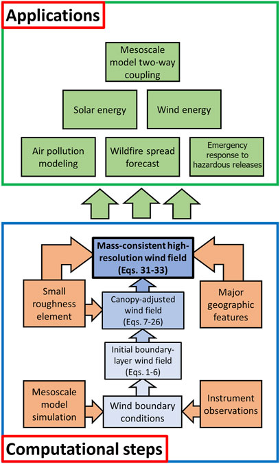
FIGURE 2. QCM computational framework. It takes three steps (blue arrows) to compute a 3-D mass-consistent wind field constrained by environmental conditions (in orange). This fast and versatile approach is used for a large range of applications (in green).

Throughout the article, we used index notation and denoted u₁, u₂, and u₃ the wind components in the x₁, x₂, and x₃ directions (respectively, easterly, northerly, and vertical). The horizontal wind speed is described with $s={(u_i{u}_i)}^{\frac{1}{2}}$, for i = 1, 2. For a given variable Φ, we noted Φⁿ, the nth observation, Φ⁰, the initial-guess, and Φ^f the final value field.

2.1 Boundary-layer wind

2.1.1 Initializing the wind field

The fast-response model QUIC can readily simulate 3-D wind fields in urban or flat terrain from different types of wind data, including single observation data points, vertical profiles, or other models. After reading in observation wind magnitude and direction (both horizontal wind components, $u_1^n$ and $u_2^n$), and their location in space, the horizontal wind field is initialized in two steps. For each input wind data n at a given location $(x_1^n,x_2^n)$, the vertical profile of the horizontal wind speed $s^n={(u_i^n{u}_i^n)}^{\frac{1}{2}},i=\mathrm{1,2}$, is computed using Monin and Obukhov (1954) similarity theory (MOST). These profiles are then assimilated into a 3-D wind field with the Barnes (1973) method. It is recommended to have at least three initial data points for accurate interpolation. In QUIC, MOST wind profiles are defined as

$s^n\left(x_3\right)=\frac{u_{*}}{\kappa }\left(\ln \left(\frac{x_3}{z_0}\right)+{\mathrm{\Phi }}_m\left(\frac{x_3}{L}\right)\right),(1)$

with κ, the Von Karman constant, u_*, the friction velocity, z₀, the aerodynamic roughness, x₃/L, a dimensionless stability parameter, Φ_m, the stability function (Businger et al., 1971), and the Obukhov length, L, defined as

$L=-\frac{u_{*}^3{\bar{\theta }}_v}{\kappa g{\left(\overline{u_3^{\prime }{\theta }_v^{\prime }}\right)}_s},(2)$

with ${\bar{\theta }}_v$, the mean virtual temperature, g, the gravitational acceleration, and ${(\overline{u_3^{\prime }{\theta }_v^{\prime }})}_s$, the surface virtual potential temperature flux. We used the standard notation for the decomposition into mean and perturbation elements such that, for a given variable ϕ, we have = $\varphi =\bar{\varphi }+{\varphi }^{\prime }$.

u_* is determined by evaluating Eq. 1 at the lowest wind measurement available at $(x_1^n,x_2^n)$, ideally unaffected by terrain roughness elements. The aerodynamic surface roughness, z₀, is estimated from the type of land cover underlying the forest, since canopy effects are only considered later on. Typically, it varies from 10^–2 m above flat terrain to 10^–1 m above crops (e.g., Silva et al., 2007). x₃/L and Φ_m reflect the impact of atmospheric stability on the wind profile and can be computed from vertical gradients or fluxes of velocity and temperature records, as shown in the equation above (Arya, 2001). In the absence of data, we assume neutral stability and Φ_m = 0.

Subsequently, the 3-D horizontal wind field s⁰ is constructed in two passes using a Barnes interpolation scheme (Barnes, 1973). Firstly, an intermediate wind field, s′⁰, is estimated as

$s^{\prime 0}=\frac{{\displaystyle {\sum }_n}{\omega }^n{s}^n}{{\displaystyle {\sum }_n}{\omega }^n},(3)$

and, in a second time,

$s^0=s^{\prime 0}+\frac{{\displaystyle {\sum }_n}{\omega }^{\prime n}\left(s^n-s^{\prime 0}\right)}{{\displaystyle {\sum }_n}{\omega }^{\prime n}}.(4)$

Here, ωⁿ and ω′ⁿ are exponential weight parameters defined as functions of the distance between each grid point and wind data location within a given radius (tens to thousands of kilometers depending on the domain size). More precisely, they are defined as

${\omega }^n=\exp \left(-\frac{1}{\mathrm{\Lambda }}\mathrm{\Delta }\right),(5)$

and,

${\omega }^{\prime n}=\exp \left(-\frac{1}{\gamma \mathrm{\Lambda }}\mathrm{\Delta }\right),(6)$

with $\mathrm{\Lambda }=5.052{\left(2\frac{\overline{{\mathrm{\Delta }}^n}}{\pi }\right)}^2$, an estimation of the wind wavelength (Koch et al., 1983), $\overline{{\mathrm{\Delta }}^n}$, the average distance between each data point, γ = 0.2, a parameter controlling the level of detail (e.g., a smaller value would correspond to a better rendition of short wavelengths), and $\mathrm{\Delta }={(x_i^n-x_i)}^2$, the squared distance between a data point and a grid point. The scheme is designed to work well with unevenly distributed or sparse observations, e.g., coarser NWP simulation results or a limited number of ground-based instrumentation.

2.1.2 QUIC data assimilation

As mentioned earlier, the QCM model can be initialized from observation data or other simulation models results. In the present study, we used an offline one-way coupling between the NWP model WRF and QCM. WRF often rely on staggered grids for which the wind velocity components are resolved on the cell faces rather than at the center. To avoid an extra interpolation at the cell center that could result in data loss, QUIC independently computes the first-guess wind fields for $u_1^0$ and $u_2^0$ onto the same final grid. For each input data point, $u_1^n$ and $u_2^n$, the elevation above ground level (AGL) is computed by dividing the sum of the base-state and perturbation geopotential (computed by WRF) by the gravitational acceleration, g. Since the NWP domain simulations typically generate results over millions to billions of cells, the number n_WRF of WRF input points used for the QCM initialization is set as a model parameter to better study the impact of the input resolution on the final wind field accuracy. Depending on that parameter and others specified in Section 3.2, the QCM selects different sets of n_WRF WRF data points such that they cover the domain as homogeneously as possible. In Section 4.2, we show how this parameter only slightly impacts the QCM results. WRF simulations using LUC to model the woods and forests’ influence are unlikely to accurately model the impact of small forest patches on the wind flow, especially near the ground, without using canopy sub-models such as Arthur et al. (2019); Ma and Liu (2019). In that case, the QCM is expected to deliver more accurate results at a higher resolution.

At a given horizontal location, $(x_1^n,x_2^n)$, for which a data point is selected as input, the wind profiles for both the $u_1^n$ and the $u_2^n$ components are defined by Eq. 1. The friction velocity is computed for the lowest WRF data point available at that location, preferentially far enough above the canopy. Above the highest WRF data point, the profile is extrapolated from a gradient defined by the progression of the data at the closest available altitude levels. Using a cubic spline, the vertical profile is parameterized at each point located between the lowest and highest points. Finally, the first-guess horizontal wind field s⁰ is computed by assimilating $u_1^n$ and $u_2^n$ simultaneously into the same 3-D computational domain, following the method developed in Section 2.1.1.

2.2 Canopy-adjusted wind

2.2.1 Background

The canopy wind is computed in the QCM from atmospheric stability, vegetation cover height and density, and boundary-layer wind data taken above the canopy. An important element of our model is its capacity to simulate sub-canopy jets (SCJ). Before deriving the model equations, we review our current understanding of the canopy wind patterns to identify how this phenomenon arises. In the next Section 2.2.2, we derive the canopy wind model and determine what hypothesis leads to more accurate results in modeling the SCJ and the other prominent features of the mean canopy wind.

Boundary-layer winds are affected by the presence of vegetation below about two to three times the canopy height (Brunet, 2020), namely, in the roughness sublayer (RSL). This range of values corresponds to a theoretical limit commonly reported in the literature, but alternative definitions accounting for the atmospheric conditions and variations in canopy density indicate that the RSL height may be up to five times the canopy height (Thomas et al., 2006). The mixing-layer analogy is commonly used Raupach et al. (1996) to understand these interactions between the surface layer and the canopy layer. In short, plant elements absorb momentum from above, and an inflection point develops near the canopy top. The inflection sustains the development of Kelvin-Helmholtz instabilities, which evolve into spanwise roller vortices. These vortices may extend and stretch into 3-D coherent mixing-layer-like structures or form pairs of head-up and head-down vortices sustained by the strong asymmetric shear (Bailey and Stoll, 2016). The strong decrease in momentum at the canopy top leads to a characteristic exponentially decreasing wind profile just below. Quadrant analyses (e.g., Guan et al., 2018) help to explain the momentum distribution within the canopy. Upward ejections (s′ < 0 and $u_3^{\prime }>0$) are the most commonly observed events, and downward sweeps (s′ > 0 and $u_3^{\prime }<0$) transport the most momentum across the canopy layer. In a forest with a low plant density near the ground, the momentum flux advected by sweeps is not completely absorbed before reaching the ground, and a SCJ may form (see, for example, Grant et al., 2015). The relevant atmospheric wind layers, wind momentum, and wind speed profiles are available in Figure 3.

FIGURE 3

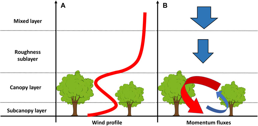
FIGURE 3. Schematic illustrating (A) average canopy wind speed profile and (B) momentum transfer in and above the canopy layer. (A) Shows that, at approximately three times the tree height, in the mixed layer, the wind is unaffected by the canopy. Below, in the roughness sub-layer, the wind profile is commonly approximated by a displaced logarithmic wind profile (the displacement height is a function of physical parameters such as LAI, drag coefficient, and tree height). The wind speed within the forest is attenuated, logarithmically proportional to the density of plant elements. A sub-canopy jet can be observed close to the ground when the sub-canopy vegetation is sparse and the trees sufficiently tall. (B) Shows that the downward fluxes in the mixed layer and the roughness sub-layer carry momentum from the overlying flow to the top of the canopy layer. The vegetation absorbs a large part of that momentum and typical turbulence structures appear near the canopy top (Bailey and Stoll, 2016). As a result of these complex interactions, sweeps (in red), and ejections to a lesser extent (in blue), dominate the turbulent momentum balance and cause an injection of momentum in the lower sub-canopy layer. A sub-canopy jet may form as a consequence of this non-local contribution.

Modeling the complex turbulent canopy wind structures is beyond the scope of this work. However, it is possible to simulate the most prominent features of the canopy flow, like the SCJ, wind attenuation within the canopy, or displaced logarithmic profile above, thanks to a mean wind model derived from the Navier-Stokes equations. The following subsection derives and presents a canopy model that rapidly runs using input of vegetation density and height and wind speed above the RSL.

2.2.2 Averaged Navier-Stokes equations

Within each cell, we assume a static and horizontally homogeneous canopy over terrain with moderate slope angles (a few degrees or less). The fluid is assumed incompressible and the Coriolis effects negligible. The momentum equations may then be written as

$\frac{\partial u_i}{\partial t}+\frac{\partial u_i{u}_j}{\partial x_j}=-\frac{1}{\rho }\frac{\partial P}{\partial x_i}+\nu \frac{\partial }{\partial x_j}\frac{\partial }{\partial x_j}{u}_i.(7)$

As mentioned earlier, u_i represents the ith component of the velocity vector in the x_i direction, following standard index notation. P is the thermodynamic pressure, ρ the air density, and ν the air kinematic viscosity. At higher slope angles, effects due to temperature gradients non-orthogonal to the surface play a more significant role in momentum conservation. They can be modeled by adding a buoyancy term in Eq. 7 (Oldroyd et al., 2014).

For a fast-response model, we choose to compute the ensemble- and volume-averaged wind field. Classically, the Reynolds-averaged Navier-Stokes equations are given by

$\frac{\partial {\bar{u}}_i}{\partial t}+\frac{\partial {\bar{u}}_i{\bar{u}}_j}{\partial x_j}=-\frac{1}{\rho }\frac{\partial \bar{P}}{\partial x_i}+\nu \frac{\partial }{\partial x_j}\frac{\partial }{\partial x_j}{\bar{u}}_i-\frac{\partial \overline{u_i^{\prime }{u}_j^{\prime }}}{\partial x_j}.(8)$

The overbar represents the ensemble average operator and the primes are departures from the mean. Analogously, a given model variable φ = φ(x₁, x₂, x₃, t) can be decomposed in its volume-averaged component and the variation from it: $\phi =⟨\phi ⟩+\phi \prime \prime$. The superficial volume average definition for a cell in the canopy with an homogeneous distribution of plant elements, pioneered in Raupach and Shaw (1982), is given by Schmid et al. (2019) as

$⟨\phi \left(x_i,t\right)⟩=\frac{1}{\mathcal{V}}{\int }_{{\mathcal{V}}_f}\phi \left(\left(x_i+\mathrm{d}{x}_i\right),t\right)\mathrm{d}\mathcal{V},(9)$

with $\mathcal{V}$, the cell volume, ${\mathcal{V}}_f\subseteq \mathcal{V}$, the volume occupied by fluid, $\mathrm{d}\mathcal{V}=\mathrm{d}{x}_1\mathrm{d}{x}_2\mathrm{d}{x}_3$ an infinitesimal volume element, dx_i, an infinitesimal change in x_i. In a plant canopy, the solid regions are small compared to the fluid ones such that ${\mathcal{V}}_f=\mathcal{V}$. The volume averaging operator does not necessarily commute with differentiation. Instead, we have

$⟨\frac{\partial \phi }{\partial x_i}⟩=\frac{\partial \langle \phi \rangle }{\partial x_i}+I_{{\phi }_i},(10)$

where $I_{{\phi }_i}=I_{{\phi }_i}^{S_i}+I_{{\phi }_i}^{S_0}$ is the sum of the integral of φ_i over the plant elements surface, S_i, and the outer cell surface, S₀. In what follows, we neglect the horizontal advection of φ_i across horizontal cells to assume $I_{{\phi }_i}^{S_0}<I_{{\phi }_i}^{S_i}$. If φ is constant along the interface S_i, then $I_{{\phi }_i}^{S_i}=0$ (Raupach and Shaw, 1982), and the two operators commute. Now, applying the volume averaging operator to Eq. 8 gives

$⟨\frac{\partial {\bar{u}}_i}{\partial t}⟩+⟨\frac{\partial {\bar{u}}_i{\bar{u}}_j}{\partial x_j}⟩=-⟨\frac{1}{\rho }\frac{\partial \bar{P}}{\partial x_i}⟩+⟨\nu \frac{\partial }{\partial x_j}\frac{\partial }{\partial x_j}{\bar{u}}_i⟩-⟨\frac{\partial \overline{u_i^{\prime }{u}_j^{\prime }}}{\partial x_j}⟩.(11)$

2.2.3 One-dimensional canopy wind momentum

In a static canopy, the wind remains constant (zero) along the plant elements surface S_i. Then, the two operators commute for

$\begin{array}{ll}\hfill ⟨\frac{\partial {\bar{u}}_i}{\partial t}⟩& =\frac{\partial ⟨{\bar{u}}_i⟩}{\partial t},\hfill \\ ⟨\frac{\partial {\bar{u}}_i{\bar{u}}_j}{\partial x_j}⟩\hfill & =\frac{\partial ⟨{\bar{u}}_i{\bar{u}}_j⟩}{\partial x_j},\hfill \\ ⟨\frac{\partial \overline{u_i^{\prime }{u}_j^{\prime }}}{\partial x_j}⟩\hfill & =\frac{\partial ⟨\overline{u_i^{\prime }{u}_j^{\prime }}⟩}{\partial x_j}.\hfill \end{array}(12)$

The extra surface-integral terms appearing in Eq. 10, $I_{P_i}$ and $I_{{\nabla }_i^2}$, remain only for the pressure and viscous drag force terms. Using $\frac{\partial ⟨{\bar{u}}_i{\bar{u}}_j⟩}{\partial x_j}=\frac{\partial }{\partial x_j}\left(⟨{\bar{u}}_i⟩⟨{\bar{u}}_j⟩+⟨{\bar{u}}_i^{\prime \prime }{\bar{u}}_j^{\prime \prime }⟩\right)$, and substituting Eqs 10, 12 into (11), we obtain

$\begin{array}{cc}\hfill & \frac{\partial ⟨{\bar{u}}_i⟩}{\partial t}+\frac{\partial }{\partial x_j}\left(⟨{\bar{u}}_i⟩⟨{\bar{u}}_j⟩+⟨{\bar{u}}_i^{\prime \prime }{\bar{u}}_j^{\prime \prime }⟩\right)\hfill \\ \hfill & =\left(\frac{1}{\rho }\frac{\partial ⟨\bar{P}⟩}{\partial x_i}+I_{P_i}\right)+\nu \left(\frac{\partial }{\partial x_j}\frac{\partial }{\partial x_j}⟨{\bar{u}}_i⟩+I_{{\nabla }_i^2}\right)-\frac{\partial ⟨\overline{u_i^{\prime }{u}_j^{\prime }}⟩}{\partial x_j}.\hfill \end{array}(13)$

Details of the physical meanings of each term are available in Brunet (2020). Further hypotheses are required to simplify Eq. 13 and establish a fast canopy wind model. If we assume that the ensemble- and volume-averaged momentum is conserved along the fluid particle trajectories, then

$\frac{D\langle {\bar{u}}_i\rangle }{Dt}=\frac{\partial ⟨{\bar{u}}_i⟩}{\partial t}+\frac{\partial ⟨{\bar{u}}_i⟩⟨{\bar{u}}_j⟩}{\partial x_j}=0.(14)$

Equation 13 can be divided into its kinematic and dynamic components. The rate of exchange of momentum due to the air motion is modeled by the volume-averaged kinematic momentum flux τ_ij as

$\frac{\partial {\tau }_{ij}}{\partial x_j}=-\frac{\partial }{\partial x_j}\left(⟨\overline{u_i^{\prime }{u}_j^{\prime }}⟩+⟨{\bar{u}}_i^{\prime \prime }{\bar{u}}_j^{\prime \prime }⟩\right)+\nu \frac{\partial }{\partial x_j}\frac{\partial }{\partial x_j}⟨{\bar{u}}_i⟩.(15)$

Terms on the right-hand side of Eq. 15, are turbulent, dispersive, and molecular stress components, respectively. The aerodynamic drag (Shaw, 1977), due to pressure and viscous forces fluctuations imposed by the canopy, is modeled as

$I_{P_i}+I_{{\nabla }_i^2}=-C_{d}A⟨{\bar{u}}_i⟩|\langle \bar{u}\rangle |,(16)$

with A, the leaf area density (LAD), and the drag coefficient C_d = 0.2 (identical to Massman (1997), which is the typically used coefficient value). C_d measures the effectiveness of canopy elements in absorbing wind momentum. Finally, $|⟨\bar{u}⟩|=\sqrt{⟨{\bar{u}}_i⟩⟨{\bar{u}}_i⟩}$.

Using Eqs 14–16 and neglecting the pressure perturbation gradient in Eq. 13 gives

$\frac{\partial {\tau }_{ij}}{\partial x_j}=C_{d}A⟨{\bar{u}}_i⟩|\langle \bar{u}\rangle |.(17)$

In order to simplify the tensor components, we made two assumptions. First, based on experimental observations (Raupach et al., 1986), we assumed that spatially averaged flow properties in dense canopies are to a good approximation functions of x₃. Then, we assumed that the wind direction remained equal to that at the reference point along the profile. Therefore, Eq. 17 solved for the ensemble and spatially-averaged horizontal wind speed, $⟨\bar{s}⟩$, simplifies to the 1-D canopy wind momentum equation,

$\frac{\mathrm{d}\tau }{\mathrm{d}{x}_3}=C_{d}A{⟨\bar{s}⟩}^2.(18)$

In this context, the term τ represents the shear stress tensor coefficients acting in the horizontal wind direction on a plane normal to the vertical axis.

2.2.4 Turbulent stress modeling

In the original work of Boussinesq (1877), the turbulent stress was parameterized with the eddy-viscosity K such that: $\tau =K\frac{\mathrm{d}⟨\bar{s}⟩}{\mathrm{d}{x}_3}$. This formulation only accounts for small-scale (local) transport. Yet, canopy sweeps are hypothesized to lead to non-local transport of momentum into the canopy and a secondary wind speed maxima close to the ground (Guan et al., 2018, and illustrated in Figure 3). This phenomenon is clearly noticeable in numerous other studies (Shaw, 1977; Su et al., 2008). To account for this effect, a new variable C_NL can be introduced, yielding

$\tau =K\frac{\mathrm{d}⟨\bar{s}⟩}{\mathrm{d}{x}_3}+C_{NL}.(19)$

The term C_NL represents the non-local advection of momentum, derived from the wind-shear intensity within the RSL. Here, we follow the definition of C_NL proposed by Zeng and Takahashi (2000),

$C_{NL}=C_1⟨{\bar{s}}_{\mathit{ref}}⟩\left(⟨{\bar{s}}_{\mathit{ref}}⟩-⟨\bar{s}⟩\right)\frac{x_3}{H}\exp \left\{-LA{I}_{x_3,H}\right\},(20)$

with C₁ = 0.01, a model coefficient obtained from numerical experiments of flow over corn fields, H, the local forest patch height, $LA{I}_{x_3,H}={\int }_{x_3}^H{C}_{d}A\mathrm{d}{x}_3$, the leaf area index (LAI) down to a specific depth x₃ multiplied by the drag coefficient C_d, and $⟨{\bar{s}}_{\mathit{ref}}⟩=s^0(x_{3,ref})$, the first-guess wind velocity from Eq. 4 defined at a reference height x_3,ref above the RSL. Equation 20 links the transport of surface layer momentum into the canopy to the advection of wind from the top of the RSL, and assumes that it is gradually absorbed by the canopy elements.

The eddy-viscosity, K, in Eq. 19 is defined by Prandtl (1932) as

$K=l^2\frac{\mathrm{d}⟨\bar{s}⟩}{\mathrm{d}{x}_3}.(21)$

The term l is a mixing length based on a traditional canopy-layer length scale, κ(x₃ − d), with modifications to account for stability above the canopy height so that

$l\left(x_3\ge H\right)=\frac{\kappa \left(x_3-d\right)}{{\mathrm{\Phi }}_m},(22)$

with d, the displacement height, or the mean level of momentum absorption in the canopy. The displacement height can be computed from LAD data following Raupach (1994) as

$d=H\left(1-\frac{1-\exp \left\{-\sqrt{7.5LAI}\right\}}{\sqrt{7.5LAI}}\right),(23)$

with LAI = ∫Adx₃. Within the canopy, the mixing length is defined following a definition similar to Zeng and Takahashi (2000),

$l\left(x_3<H\right)=\frac{\kappa x_3}{1+C_0{C}_{d}A{x}_3},(24)$

where C₀ is an empirical coefficient in the original Zeng’s model. Here, we compute it by assuming continuity of the mixing length at the canopy top. Setting Eqs 22, 24 equal at x₃ = H, we find

$C_0=\frac{\left({\mathrm{\Phi }}_m\left(H/L\right)-1\right)+d/H}{C_{d}A\left(H\right)\left(H-d\right)}.(25)$

Other models for the displacement height and the mixing length were implemented and tested (see Supplementary Material SA1).

2.2.5 Non-local canopy wind momentum

For a very sparse canopy, A, LAI, and d tend towards zero, such that Eqs 22, 24 define a mixing length for the mean wind similar to the classical logarithmic MOST profile extending from a few cells above the ground level to the top of the domain. In high LAD cases the mean wind speed rapidly reduces to zero within the canopy, and the logarithmic profile is observed closer to the canopy top. This is equivalent to solving the displaced logarithmic profile with a large displacement height value. Besides these limiting cases, the wind profile is mainly controlled by the LAD distribution and the non-local momentum transport magnitude. It is rarely logarithmic but rather resembles a profile similar to the one shown in Figure 3B. Finally, we use Eqs 19–21 with Eq. 18, and obtain the QCM canopy flow equation,

$\begin{array}{ll}\hfill & \frac{\mathrm{d}}{\mathrm{d}{x}_3}\left({\left(l\frac{\mathrm{d}⟨\bar{s}⟩}{\mathrm{d}{x}_3}\right)}^2\right)+C_1⟨{\bar{s}}_{\mathit{ref}}⟩\left(⟨{\bar{s}}_{\mathit{ref}}⟩-⟨\bar{s}⟩\right)\times \frac{x_3}{H}\exp \left\{LA{I}_{H,x_3}\right\}\hfill \\ \hfill & =C_{d}A{⟨\bar{s}⟩}^2.\hfill \end{array}(26)$

Equation 26 is solved numerically for the mean horizontal wind velocity vertical profile, $⟨\bar{s}⟩$, at each grid location, (x₁, x₂, x₃), x₃ ∈ [0, x_3,ref]. Above x_3,ref, the wind remains identical to the first-guess wind field described in Section 2.1. Below the reference height, the two horizontal wind components, $(⟨{\bar{u}}_1⟩,⟨{\bar{u}}_2⟩)$, are computed from the wind speed $⟨\bar{s}⟩$ above, and the first-guess wind direction value at (x₁, x₂, x_3,ref).

To solve Eq. 26, each term is explicitly differentiated and discretized using an order-1 explicit scheme with a semi-step precision and a functional, $\mathcal{F}$, is defined as $\mathcal{F}(⟨\bar{s}⟩)=0$. The tridiagonal system, $\mathcal{J}\mathrm{d}⟨\bar{s}⟩=\mathcal{F}$, is solved using the Thomas algorithm (Weickert et al., 1998) for $\mathrm{d}⟨\bar{s}⟩$, with $\mathcal{J}=\mathcal{J}(\mathcal{F})$, the Jacobian matrix. Then, $⟨\bar{s}⟩$ is updated with $\mathrm{d}⟨\bar{s}⟩$ and the linear system is solved until convergence. This procedure can be done in parallel throughout the domain since every canopy wind profile is solved independently. The vertical wind profiles computed at every grid location form the 3-D, canopy-adjusted, initial wind field and overwrite the boundary-layer flow computed from WRF simulation results or instrument observations. After this step, $u_i^0$ refers to the canopy-adjusted values for u_i, instead of the first-guess values (Section 2.1.1).

2.2.6 Massman’s and Cionco’s approaches

The QCM makes use of the vertical distribution of plant elements and parameterizes the local momentum counter-gradient effects with a non-local turbulent transfer coefficient (Zeng and Takahashi, 2000). The simulation results are compared with the original canopy wind implementation in QUIC, based on the Cionco (1965) model, and against an implementation of the Massman et al. (2017) model. The Cionco’s canopy wind model is still used for fast-modeling applications (Cionco et al., 1999), despite its simplicity. It relies on the LAI and an empirical attenuation coefficient, a (table of values in Cionco, 1972), and it does not consider the vertical variation in vegetation density. When the coefficient a is chosen carefully, the Cionco’s model manages to yield very plausible canopy wind values. The equation for the horizontal wind-aligned velocity component can be obtained by solving the 1-D momentum equation, Eq. 18, using a first-order closure model as in Eqs 19, 21, but without non-local effects (i.e., C_NL = 0), and assuming a mixing length and LAD that are constant with elevation

$s\left(x_3\right)=s\left(H\right)\exp \left\{\mathrm{a}\left(x_3/H-1\right)\right\}.(27)$

This approach reproduces the strong inflection below the canopy top thanks to the exponential formulation, but it does not converge to zero at the ground surface. It performs well within vertically homogeneous canopies, such as the corn or rice fields for which it was developed, but can be inaccurate when the underlying assumptions (e.g., constant drag with height) are violated.

The Massman’s method is based on an integrated plant area density (PAD) that varies with height. It is faster than the non-local solver, which is iterative, because it only solves a 1-D analytical expression that is based on a first-order turbulence closure Albini (1981). The resulting profile is a combination of a strongly attenuated wind near the canopy top s_t, and a simple logarithmic profile near the ground s_b which does not consider potential non-local momentum transfers. The wind profile is defined as

$s\left({\tilde{x}}_3\right)=s_b\left({\tilde{x}}_3\right)s_t\left({\tilde{x}}_3\right),(28)$

with ${\tilde{x}}_3=x_3/H$, the non-dimensional height, and

$\begin{array}{cc}\hfill s_b\left({\tilde{x}}_3\right)=\frac{\log \left({\tilde{x}}_3/{\tilde{z}}_0\right)}{\log \left(1/{\tilde{z}}_0\right)},& {\tilde{z}}_0<{\tilde{x}}_3<1,\hfill \\ \hfill 0,& {\tilde{x}}_3\ge 1,\hfill \end{array}(29)$

and,

$s_t\left({\tilde{x}}_3\right)=\frac{\cosh \left(N\zeta \left({\tilde{x}}_3\right)/\zeta \left(H\right)\right)}{\cosh \left(N\right)}.(30)$

Here, ${\tilde{z}}_0=z_0/H$, N is a model coefficient that is a function of the friction velocity and wind speed at canopy top, and $\zeta ({\tilde{x}}_3)$ is the cumulative canopy drag area (Massman, 1997). Because it relies on variables and model coefficients defined continuously within the canopy and at the canopy top, the final result is more realistic than those from the Cionco’s model. Unlike the model shown in this study, the Cionco’s and Massman’s models require prior knowledge of the wind at the canopy top, whereas the QCM can run from wind data generated from the first-guess wind field, with a reference level far above the canopy.

2.3 Mass-consistent wind model

Data assimilation and correction schemes carry uncertainties that can be minimized by enforcing mass consistency over the simulation domain. The variational analysis developed by Sasaki (1970) and refined by Sherman (1978) keeps the final wind field $\left(u_1^f,u_2^f,u_3^f\right)$ as close as possible to the canopy-adjusted wind field, $\left(u_1^0,u_2^0,u_3^0\right)$, computed in the previous section, while enforcing mass conservation. The resulting mass-consistent wind field also demonstrates upstream acceleration and downstream deceleration over small obstacles or flow channeling in canyons and narrow valleys, for an increased accuracy over weakly complex terrain that could not be achieved by the original QUIC model (defined for flat urban environments). These terrain-induced effects are more noticeable over steep slopes and abrupt elevation changes. Notably, the variational analysis attenuates the differences in wind speed between neighboring cells resulting from the canopy wind being modeled independently at each grid location.

Details of the mass-consistent flow solution process used herein are available in Bozorgmehr et al. (2021), therefore only the main steps are summarized here. We start by defining a cost function J,

$J={\int }_{{\mathcal{V}}_0}\left[{\alpha }_{x_i}^2{\left(u_i^f-⟨{\bar{u}}_i^0⟩\right)}^2+\lambda \frac{\partial u_i^f}{\partial x_i}\right]\mathrm{d}{\mathcal{V}}_0,(31)$

with ${\alpha }_{x_i}$, the Gaussian moduli, λ, the Lagrange multipliers for finding the function extrema, and ${\mathcal{V}}_0$, the domain volume. The ratio of the moduli controls the correction made in the horizontal and vertical directions during that last computational step. Generally, the horizontal contributions are the same in both x₁ and x₂ directions: ${\alpha }_{x_1}={\alpha }_{x_2}$. Here, we also assumed $\frac{{\alpha }_{x_1}}{{\alpha }_{x_3}}=1$ such that no additional correction is performed besides enforcing mass conservation. The Lagrange multipliers are obtained by solving the Poisson equation,

$\frac{{\partial }^2\lambda }{\partial x_1^2}+\frac{{\partial }^2\lambda }{\partial x_2^2}+{\left(\frac{{\alpha }_{x_1}}{{\alpha }_{x_3}}\right)}^2\frac{{\partial }^2\lambda }{\partial x_3^2}=-2{\alpha }_{x_1}^{2}R,(32)$

with R, the divergence of the initial wind field. Solid and fluid cells define Eq. 33 boundary conditions. Solid elements oppose the wind movement, so $\frac{\partial \lambda }{\partial x_i}=0$ across horizontal or vertical faces. Inlet and outlet surfaces have boundary conditions given by λ = 0. Finally, J is minimized over ${\mathcal{V}}_0$ under a physical constraint given by the continuity equation. The final solution for $u_i^f$ is

$u_i^f=u_i^0+\frac{1}{2{\alpha }_{x_i}^2}\frac{\partial \lambda }{\partial x_i}.(33)$

3 Validation cases

3.1 CHATS - Full-scale idealized homogeneous canopy

3.1.1 Environmental conditions

A series of measurements were made during the Canopy Horizontal Array Turbulence Study (CHATS, Patton et al., 2011), which investigated the wind field in a walnut orchard near Cilker Orchards, CA, between March 15 and 12 June 2007. The areas surrounding CHATS and our simulation domain are shown in Figure 4. The orchard extends over 0.64 km² of flat terrain. The canopy is quasi-homogeneous, with trees regularly spaced every 7 m, reaching a uniform height (10 m). Leaves grew between April 14 and May 13, during which the LAI increased threefold (from 0.77 to 2.635). Data taken before leaf-out is referred to as BLO, while data acquired after leaf-out is ALO. Very little plant materials was observed near the ground, and therefore the sub-canopy vegetation is considered sparse and neglected in the simulations.

FIGURE 4

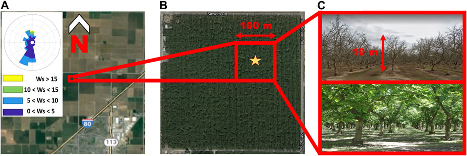
FIGURE 4. (A) and (B) satellite views along with (C) ground view of the CHATS walnut orchard. The windrose for every fifth percentile indicates the wind at 29 m above ground level and above the roughness sub-layer, Ws, were southerly or northerly. The simulation domain, highlighted in red in (A) and (B), was centered around the observation tower (yellow star) and far from the orchard boundaries to avoid edge effects. (C) Shows the distribution of tree elements significantly varied seasonally.

During CHATS, sonic anemometers were mounted at 13 elevation levels on a tower. The highest wind observation was made at 29 m AGL, thus above the RSL (Patton et al., 2011), and indicated dominant northerly and southerly wind directions. The atmospheric stability, determined by the inverse Obukhov length, varies throughout the diurnal cycle: unstable during the day; and stable during the night. These variations in the environmental conditions were propitious to study the changes of humidity, temperature, and velocity (Dupont and Patton, 2012), the ozone exchange (Brown et al., 2020), or the wind stationarity (Pan and Patton, 2020). For a more detailed analysis of CHATS stability regimes see Dupont and Patton (2012). The environmental conditions are summarized in Table 2, together with the model input and numerical setup described in the next two subsections.

TABLE 2

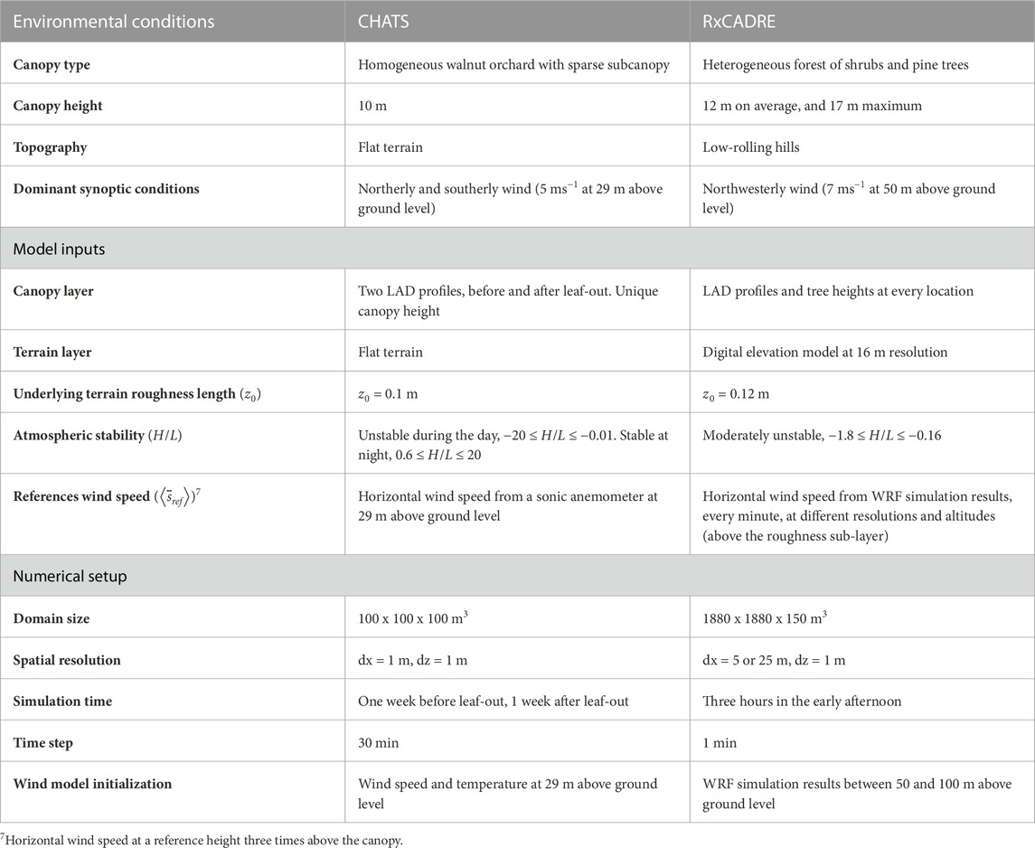
TABLE 2. Environmental conditions, model inputs, and numerical simulation setup parameters for the CHATS and RxCADRE experimental campaigns.

3.1.2 Model inputs

QUIC requires observations or simulation output to estimate the first-guess wind field and, whenever available, flux data to compute stability conditions. In the CHATS experiment, the wind measured at the top of the tower (x_3,ref = 29 m) defines the reference wind unaffected by the canopy. Velocity and temperature gradients, calculated between the two highest measurement elevation levels (23 and 29 m AGL), are used to compute the heat and momentum fluxes necessary to define the diurnally alternating stability conditions. The LAI was obtained using LI-COR LAI-2000 measurements (Patton et al., 2011). It is common to model the roughness length as a fraction of the roughness elements height (Garratt, 1992). Here, it is defined as one-10th of the canopy height (cf. Observations made by Grimmond and Oke, 1999).

3.1.3 Numerical setup

The CHATS wind fields were modeled in a 100 × 100×100 m³ domain (including 100,000 vegetation cells) with horizontal and vertical resolutions set to 1 m. Two different time periods were evaluated: a week before leaves appeared (March 25 to March 31) and a week after leaf out (June 1 to June 7). The periods used for validation were selected to maximize the amount of data available at all levels on the sonic anemometer tower. Wind velocities mostly changed during morning and evening transitions and were relatively constant throughout the day and the night, so we deemed that 30-min averages were representative enough of the simulated wind field diurnal variations.

3.2 RxCADRE - Heterogeneous forest

3.2.1 Environmental conditions

For the second validation case, we considered a 3.6 km² heterogeneous forest of longleaf pines and small bushes where winds were observed during the Combustion-Atmospheric Dynamics Research Experiments (RxCADRE, Ottmar et al., 2016a) before and during a series of prescribed burns on the Eglin Air Force Base, FL, in 2012. The terrain is moderately hilly, with slopes ranging from 1% to 5%, and the largest slopes near a stream on the northeast side of the forest. Unlike the CHATS case, the RxCADRE vegetation varies considerably and only covers parts of the simulation domain. Different species of vegetation cohabit with distinct LAD distribution and height. The LAD was estimated based on high-resolution aerial LiDAR data collected during the RxCADRE campaign using the approached described in Halubok et al. (2021). LAD was computed on a voxel grid of 5 × 5×3 m³ or 25 × 25×3 m³ (both cases are used). Figure 5 shows the heterogeneity of the domain, with tree heights ranging from 2 to 20 m AGL (12 m, on average), and LAI varying between 0.1 and 6. The canopy height and the LAI share a low positive correlation (R = 0.48). The tallest trees and densest vegetation patches are located at the southeast, northeast, and northwest corners.

FIGURE 5

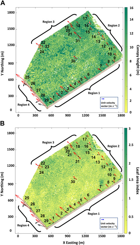
FIGURE 5. 3-h averaged wind vectors from observations (black arrows) and QCM (red arrows) interpolated to the observation height and plotted with (A) canopy height and (B) LAI, at 5-m resolution for the RxCADRE case. The vegetation density was greater in the northwest corner and along the roads (brown lines). LAI rarely exceeded 3 so the color scale was edited to reflect the heterogeneity of smaller values. The LAI and the tree height shared a low positive correlation (R = 0.48). WRF simulations were used to drive QCM to simulate wind fields every 5 min and at 5-m resolution. Results were validated against a network of anemometers (1–30) and a tower (31), divided into four regions. Region 1, near the road along the southeast border (1–9); Region 2, close to the stream on the northeast corner (10–17); Region 3, within the forest, away from edges (18–24, 30, and 31); Region 4, on the road along the southwest forest corner (25–29). Simulation results and observations frequently pointed in the same direction, except at the southeast corner, due to forest edge effects not being resolved, and at the northeast corner, possibly because of an important terrain gradient along a nearby stream bed.

Synoptic wind conditions and atmospheric stability were estimated from WRF simulations taken above the RSL. The average winds at the site were southwesterly, at 7 m s⁻¹ (Figure 1) at 50 m AGL. For the most part, atmospheric stability conditions were unstable. To validate our simulation results, we compared the results obtained from the coupled QCM-WRF simulation with those from a network of 31 cup-and-vane anemometers mounted at 3.3 m AGL that measured wind speed and direction every 3 s, and two 1-Hz sonic anemometers at 3.8 and 8.7 m height on a tower. The locations of observation instruments in the forest are plotted in Figure 5. For the rest of the study, observation locations are sorted into four geographic regions: Region 1 along a road in the woods on the southeast side; Region 2 close to a stream on the northeast side; Region 3 in the northwest part and central region of the forest; Region 4 near the road at the southwest corner. Table 2 shows a synthesis of the environmental conditions, model input and numerical setup.

3.2.2 Model inputs

The reference wind above the RSL was obtained from WRF simulation results at different resolutions and located between 50 and 100 m AGL, above the RSL (the choice for the upper boundary did not influence the results near the surface). The WRF model typically runs environmental simulations over domain cells extending over kilometers, at mesoscale levels (at least 10 km). For the RxCADRE campaign, it was run at an exceptionally high horizontal grid resolution, very close to the ground, within the RSL. Using a nested approach over seven domains, horizontal grid cell spacing were set to 12, 4, 1.33 km, 444, 148, 49, and 16 m (with a 1:3 ratio). The number of grid points ranged from 97 × 97×41 cubic cells for the first six domains, to 115 × 115×41 cubic cells for D-7 (Figure 6). The vertical grid resolution was a few tens of meters for the first ten levels, and quickly increased to 1 km at the top of the domain, around 15.2 km. The planetary boundary layer was modeled with the Yonsei University scheme (or, YSU PBL scheme, Hong et al., 2006). Surface layer physics were derived from MOST, the land-surface model came from Noah (Niu et al., 2011). The setup is exactly as described in Mallia et al. (2020).

FIGURE 6

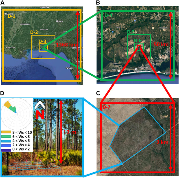
FIGURE 6. (A) to (C) nested WRF simulation domains (D-1 to D-7) for the RxCADRE campaign and (D) photograph of the forest taken at ground level. The first three domains in (A) were generated at spatial resolutions of 12, 4, and 1.3 km. For D-4 to D-7, in (B) and (C), the resolution increased threefold, until 16.5 m. The blue region in (C) corresponds to the L2F site, at which high-resolution LAD and tree height data were available. (D) Shows the tree cover was relatively sparse and the forest very heterogeneous. On the windrose, the average wind speed at 63 m, Ws, was northerly at 7 m s⁻¹, on average. Circles represent the 16th percentile.

The roughness length was estimated as in the CHATS case. The inverse Obukhov length was derived from WRF surface heat fluxes and friction velocity estimations. The canopy height is specified at 5 and 25 m horizontal resolution and vertical variation in LAD is specified every 3 m. The terrain elevation was obtained from the WRF dataset at 16 m resolution and linearly interpolated to 5 and 25 m. LUCs were also taken from the 16 m resolution dataset and interpolated with the nearest neighbor method to the final resolution. In both cases, the minimum and maximum terrain elevation were around 15 and 45 m, respectively.

3.2.3 Numerical setup

Two QUIC simulation domains were generated at 5 and 25 m horizontal resolution to match the input LAD resolution. In both cases, the domains extended over 1,880 × 1,880×150 m³, and vertical resolution was set to 1 m. The background wind field was computed every minute, 3 h before the prescribed burn on the morning of 11 Nov 2012. WRF simulation results were assimilated at different resolutions and with different numbers of points to help determine which parameter has the most impact on the QCM-WRF coupling. Starting with a reference configuration defined as N_WRF=100 points from the highest-resolution WRF simulation, D-7, and the finest definition of LAD available at dx = 5 m, we varied the number of input WRF data points, the simulation resolution (Figure 6), or the canopy spatial resolution for the following setups.

a) N_WRF=1, located at the center of the domain.

b) N_WRF=100, evenly distributed throughout the domain.

c) N_WRF=10,000, also evenly distributed throughout the domain.

d) N_WRF=100, WRF domain is D-5 (148 m horizontal resolution).

e) N_WRF=100, WRF domain is D-6 (49 m horizontal resolution).

f) N_WRF=100, WRF domain is D-7 (16 m horizontal resolution), LAD and DEM horizontal resolution set to dx = 25 m.

To quantify error, we used an absolute and a normalized metric, the mean absolute error (MAE) and the normalized root-mean-square error (NRMSE) in Figure 7. The former is commonly used to compare results perceptible at the human scale, and the latter is the proportion of the root-mean-square error (RMSE) related to the range of the modeled variable. To provide more context, we also added a relative error metric, the mean fractional bias (MFB). The MAE, NRMSE, RMSE, and MFB errors are presented in Table 4, and discussed later in Section 4.2.

FIGURE 7

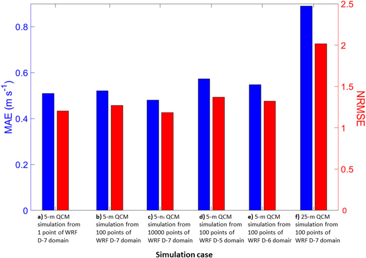
FIGURE 7. Mean absolute error (MAE, in blue) and root-mean-square error normalized by the observational variance (NRMSE, in red) of the horizontal wind speed for different simulation parameters for the RxCADRE case. (A–C) correspond to 5-m horizontal resolution simulations run from 1, 100, and 10,000 WRF D-7 domain input points. (D,E) show results for 100 input points from the D-5 and D-6 WRF domains. The errors were larger than for the D-7 cases because here the WRF simulations were generated from coarser topography and land use inputs. (F) Shows the error for a WRF simulation run with 100 points in D-7, using a LAD and tree height resolution at 25 m, was higher than the other cases. This indicates that the forest spatial resolution was a critical parameter for determining the canopy wind field accuracy in our simulations due to the vegetation heterogeneity.

4 Results and discussion

4.1 CHATS - Full-scale idealized homogeneous canopy

The orchard in CHATS evolved across the seasons (Figure 4C). While the average tree height stayed constant, the LAI increased with upper canopy leaf growth. Figure 8 indicates that, as expected, the wind speeds at all heights were stronger BLO than ALO, since there were fewer plant elements to absorb the momentum. The trees were regularly trimmed, and the volume occupied by the trunks was small compared to the total canopy volume supporting the assumption that the LAD is the most relevant parameter influencing canopy winds. Hence, the sub-canopy vegetation layer always remained sparse (the LAD from 0 to 2 m AGL was only a tiny fraction of the local maximum LAD, cf. Figure 8A). It formed an ideal configuration for the development of the SCJ (as theorized by Shaw (1977)). The canopy and the synoptic conditions were constant over the domain, and as a result all wind models gave similar results at every location except near the forest edges. The numerical scheme for the QCM converged rapidly (in ten iterations). The other canopy wind sub-models tested (Cionco’s and Massman’s) computed the canopy wind instantly since they do not rely on an iterative approach. Besides the adjustment to the complex terrain, the QCM wind-field initialization (cf. Section 2.1) and convergence towards mass-consistency only took a fraction of a second to solve on the relatively small CHATS domain. Specifically, the program run serially on a personal computer (2.30 GHz processor, 16 GB RAM) took about half a second for one time step, and less than 7 min to run 2 weeks of physical time at 30-min resolution.

FIGURE 8

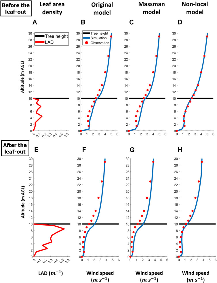
FIGURE 8. Monthly-average LAD (red line) and 1-week average horizontal wind profiles before and after leaf-out for the CHATS case. Tree height (black line) remains constant throughout the year. Before leaf-out, the LAD (A) was low because only woody plant elements were present. After leaf-out, the LAI increased threefold and the LAD (E) was five times higher near the canopy top. The wind profiles (in blue) of the original model (B,F), the Massman’s model (C,G), and the current QCM (D,H), are plotted against observations (red dots) in the last three columns.

Seasonal variation was the most important factor in determining the wind profiles. Figure 8 shows the one-week-averaged observed and simulated horizontal wind magnitude for the different evaluated wind models. In both cases, a low-level secondary maximum was observed in the sub-canopy layer. BLO, all models resulted in good wind attenuation near the canopy top and magnitude close to the ground, but for different reasons (Figures 8B–D). The Cionco’s model relies on an empirical attenuation coefficient (cf. Cionco, 1972) that controls the exponential reduction in wind speed below the canopy top. Above the canopy, the wind follows a displaced logarithmic profile shape. In the original QUIC model, both wind profiles are combined by requiring that their derivative matches at the canopy top, and this is done by slightly adjusting the displacement height of the logarithmic profile above the canopy (Speckart and Pardyjak, 2014). The Massman’s approach also models the wind above the canopy with a displaced logarithmic profile, but unlike the QUIC original and new model, the derivatives are not matched and it remains discontinuous at the canopy top. Within the canopy, the wind profile is a function of the integrated plant density and a logarithmic function parameterizing the wind near the ground. This model assumes that vegetation layers gradually absorb the vertical wind momentum, until the wind speed reaches zero at ground level. Thus, it cannot reproduce secondary wind maxima. The QUIC non-local canopy model performs better because it accurately predicts the SCJ magnitude and computes the wind within and above the canopy with a single equation (and different boundary conditions at top). This approach yields a more continuous wind profile near the canopy top than Massman’s model, and the wind speed is more attenuated in denser canopy layers than Cionco’s and Massman’s models results. ALO (Figures 8E–H), the observed wind speed was highly impacted and decreased much faster with depth into the canopy. The observed SCJ was also weaker than BLO. The Cionco’s and Massman’s models still overestimated the horizontal wind, and could not predict its speed at canopy top as accurately as BLO. The QCM consistently overestimated the wind speed but outperformed the Cionco’s and Massman’s models at almost all levels. These better results can be explained by the greater heterogeneity in the vertical distribution of LAD, favoring the application of the non-local canopy wind solver.

General model performances across seasons are presented in the scatter plots in Figure 9. Simulation results defined every meter starting from x₃ = 0.5 m were linearly interpolated to the observation elevation level. Pairs of observation and simulation data points were randomly selected to offer an overall comparison at different times and heights representative of the simulation. For cases occurring BLO, the Massman’s model (Figure 9B) had the largest departure from observations both within and above the canopy, followed closely by the original model (Figure 9A). These results confirm that both models did not resolve the SCJ and underestimated the canopy attenuation, as observed in Figure 8. The QCM (Figure 9C) results were generally within 25% of observations. ALO, both the Massman’s (Figure 9E) and the original (Figure 9D) models displayed a bias that was often 25% more than the observed wind speeds, for the same reasons discussed for BLO. The QCM (Figure 9F) also overestimated the wind speed but the error spread was smaller. It is worth noting that all models performed well for high wind speeds above the canopy. At that altitude, near the top of the RSL, the wind speed were nearly independent from the forest-induced attenuation and the displaced logarithmic models were accurate.

FIGURE 9

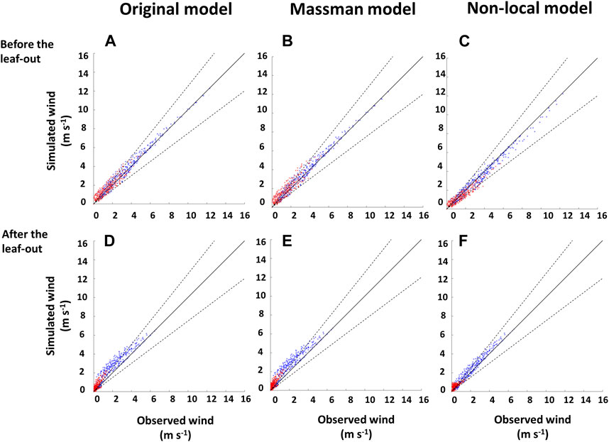
FIGURE 9. Randomly selected wind magnitude observations against simulation results before leaf-out (A–C), after leaf-out (D–F) for the CHATS case (for 50 instantaneous time moments). Red dots and blue circles represent values below and above the canopy top, respectively. The central black diagonal line denotes a 0% error between model results and observations; black dashed lines represent a 25% deviation from it. The wind speed attenuation within the canopy was weaker before leaf-out for all models. The original model and the Massman’s model overestimated the measured wind speed, and the new non-local model underestimated it.

Aside from changes in vegetation density, diurnal cycles play an essential role in defining the average wind profile and atmospheric stability conditions. Figure 5 in Brunet (2020) provides a comprehensive diagram illustrating how the mechanisms of canopy wind (as detailed in Section 2.2.1) change under stable, near-neutral, and unstable atmospheric conditions across various vegetation densities. In short, the attenuation of wind momentum through the canopy is weaker during unstable conditions because the mean flow is driven by the rising buoyant plumes rather than the mean shear, and the inflection near the canopy top is stronger in stable conditions, as the buoyancy acts to damp the vertical momentum transfer. As a result, the most effective wind momentum transport tends to occur during neutral conditions. In QCM, the stability effects are integrated in the definition of the first-guess wind field. The most significant influences modeled are the reproduction of faster wind from a reference height, driven by larger temperature gradients during daytime (after sunrise and before sunset), and vice versa at night. Observations and simulation results for the daytime and nighttime time periods are compared in Figure 10.

FIGURE 10

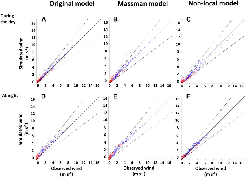
FIGURE 10. Similar to Figure 9, for wind observations and simulations results during daytime (A–C) and at night (D–F) for 25 moments before and 25 moments after leaf-out. Typically, the wind speed was greater during the day due to stronger synoptic winds. All models overestimated the wind speed at night.

Every model yielded better results during the day than at night. The original model (Figure 10A) and Massman’s model (Figure 10B) still overestimated the wind speed, but gave mostly accurate results above the canopy. Most wind model simulations showed a more significant departure from the observations near the ground, in particular at night. It likely happened at times when stability acted more strongly against the conveyance of wind momentum through the canopy. The QCM (Figure 10C) yielded better results than the two other canopy models, but underestimated the high wind speed values above the canopy and overestimated the lowest wind events within the canopy. In some cases, Massman’s model and QCM also underestimated the low wind speed events (near the ground level). It could be caused by thermodynamically-driven energy exchanges driving a very local increase in wind speed, an effect not resolved by momentum equation solvers. At night, the original model (Figure 10D) and Massman’s model (Figure 10E) displayed a clear 25% overestimation, except for the strongest winds above the canopy. In this case too, the QCM (Figure 10F) has better agreement with measurements. Since the QCM was the only model that explicitly solves for the SCJ observed at that location, it was the best-performing model overall.

Table 3 shows an absolute and a relative error metric, the bias and the RMSE during four environmental conditions with different configuration of daytime, nighttime, before and after leaf-out periods. The simulation results are linearly interpolated to the anemometer tower observations’ elevation (Figure 4). Both metrics confirmed the good performance of the QCM. In every case, the errors were at least two times smaller for the QCM results, compared to the two other models. The best results for the QCM bias and the RMSE were realized during daytime, ALO, and at night, BLO. It means the model performed similarly well independently of environmental conditions. The Cionco’s and Massman’s models consistently overestimated the observed wind speed, as observed in Figure 8, with better results for both error metrics ALO.

TABLE 3

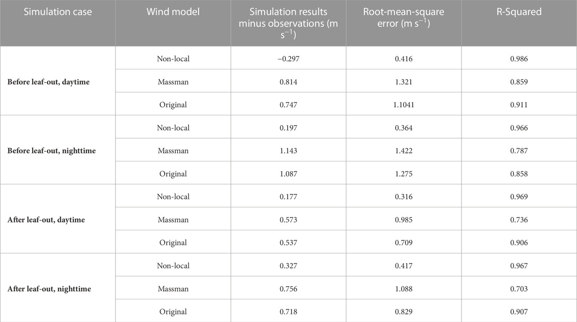
TABLE 3. Error statistics for three models in four different environmental conditions during the CHATS experiment at all heights and times. The first and third simulation cases correspond to results recorded after sunrise and before sunset from March 25 to March 31, and from June 1 to June 7, respectively. The second and fourth cases correspond to the rest of the time during these 2 weeks.

4.2 RxCADRE - A heterogeneous forest

The RxCADRE validation case lasted 3 h and covered a much more heterogeneous forest site than the CHATS case (Section 4.1). The LAD varied in both horizontal and vertical directions, with several types of plants sharing a cell location. The large forest site (named L2F, cf. Figure 1B in Ottmar et al., 2016a) was bordered by a stream on the northeast side, and dirt roads on the southeast, southwest, and northwest corners (Figure 5). The canopy layer was defined from ground level to an effective height observed by LiDAR. Out of the forested part of the domain, QUIC simulated a logarithmic profile as a function of the roughness length, stability, and synoptic conditions. Effects due to forest edges or single tree wakes were not implemented here (see Margairaz et al., 2022, for a model implemented in QES-WINDS). As discussed in Section 2.1.2, QUIC can assimilate WRF data at different resolutions to define a first-guess wind field. The nested domain approach for the RxCADRE case, introduced in Section 3.2.3 and presented in Mallia et al. (2020), proved successful in improving wind results over and within the L2F canopy, when implementing the Massman’s model (Massman et al., 2017) in WRF-SFIRE. In this section, we compare QUIC’s original and new canopy wind models. For both cases, the wind boundary conditions were derived from WRF simulations for different environmental conditions (Table 2). At 5-m resolution, the simulation domain was comprised of more than 21 millions cells, including nearly 632,000 vegetation cells. QUIC solved the 3-D wind field in 11–12 s per time step on average, when measured on the same personal computer mentioned above. Computation of the final divergence-free wind field was the most time-consuming task (about 10 s), while the initialization and canopy adjustment (with the non-local method) took about 0.01 and 1 s each. Three hours of simulation, with 1 minute time increments, took 35 min. The initialization time increased linearly with the number of input data points, N_WRF.

Figure 5 shows the distribution of 3.3-m anemometer locations inside the L2F forest site, along with 3-h averaged QCM simulation results and horizontal wind velocity observations at those locations. The results were linearly interpolated to the observation elevation level. A simple correlation analysis showed that the wind speed decreased with increasing LAI, but was not clearly associated with the local tree height. This can be explained by observations being less affected by effects present near canopy top since its height was often several times the anemometer altitude (3.3 m AGL). Overall, the QCM performed well within and outside the canopy, but the average model performances varied from region to region. In Region 1, the southeast road was oriented in the normal direction of the synoptic wind direction, so the channeling effect was limited. Moreover, the observations were recorded close to a dense part of the forest, surrounded by 10–15-m tall trees. As a result, the canopy elements density essentially determined the wind, and the simulation results compared well with observations (except at locations 1 and 3). In Region 2, the QCM did not capture a local change in wind direction, likely due to the presence of a stream. Indeed, the stream is bordered by tall and dense vegetation and edge effects can significantly influence the wind direction in the surroundings. The difference in direction did not exceed 45°, and the wind magnitude was the most accurately reproduced in that region of the domain. Observed wind speeds were much weaker than the simulation results in Region 3. This discrepancy could be caused by underestimation of the LAD by LiDAR within the forest, where the vegetation heterogeneity made it difficult to measure accurate values even at 5-m resolution (Halubok et al., 2021, details how the heterogeneity and clumping cause a negative bias in LAD). Finally, there were no trees in Region 4 and the southwest road was aligned with the wind direction. As a result, the wind was channeled along the forest edge, and the observed wind magnitude was stronger. Since the QCM solved for mass-consistency (Section 2.3), the simulated wind field reproduced this physical phenomenon, but the unresolved variations in wind directions were likely due to forest-edge effects that were not modeled.

As synthesized in Figure 2, we noted that the QCM operates in three steps: 1) the first-guess wind field is computed by assimilating the synoptic winds through WRF; 2) the initial wind field is adjusted to account for the vegetation cover; 3) the final velocity field is forced to conserve mass and thus accounts for effects due to changes in terrain elevation across the domain. The results for (1) to (3) with the original and the new QUIC canopy model were normalized by the wind speed at x₃ = H to reinforce the contribution of each computational step, and plotted in Figure 11 against four observations. The four locations (anemometers 1, 15, 31, and 28 in Figure 5) were selected to better evaluate the impact on the wind profile of variations in LAD distribution and trees height. The normalized results for the original model based on Cionco’s work consistently yielded a exponentially decreasing wind profile, very similar at every location with vegetation elements. Indeed, the empirical attenuation coefficient a did not vary much between the different anemometer locations.

FIGURE 11

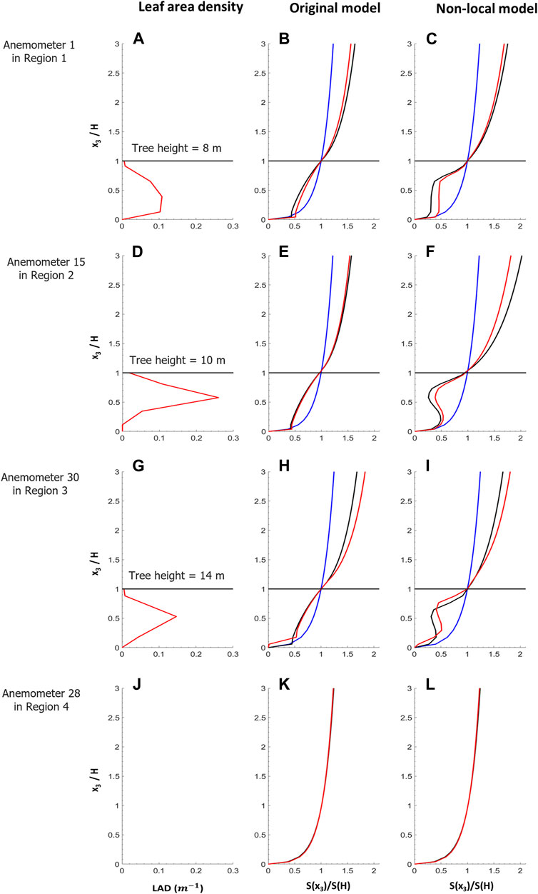
FIGURE 11. Profiles of LAD (A,D,G,J) and wind speeds computed with the original model (B,E,H,K) and QCM (C,F,I,L) for the first-guess (blue), the canopy-adjusted (black), and the mass-consistent (red) solutions for the RxCADRE case. The horizontal black line represents the average tree height. Each line corresponds to a different location in a different part of the domain. From top to bottom: location 1 in Region 1, location 15 in Region 2, location 30 in Region 3, location 28 in Region 4. There were no trees in Region 4. The wind profiles were normalized with the wind speed at the domain-average canopy height, 12 m. For the other three locations, the average tree heights were 8, 10, and 14 m, respectively. The first-guess wind profiles were always logarithmic. Profiles in (B,C,H,K) decreased exponentially within the canopy and abruptly converge to zero near the ground.

In Figures 11A–C, the sub-canopy layer was denser than the rest of the canopy, except near the top of trees. As a result, the QCM did not predict a strong SCJ. The final wind profiles were stronger than the initial ones thanks to the corrections made during step (3) to account for changes in terrain elevation in neighboring cells. In Figures 11D–I, the upper-canopy layer was distinctly denser than the sparse sub-canopy. The QCM showed a more substantial reduction in wind speed just below the canopy top than Cionco’s model results, and a more continuous decrease to zero indicative of the canopy absorbing all momentum. This result was verified for all locations within the canopy. Results in Figures 11J–L were plotted for reference purposes only. Since there was no vegetation at the last location plotted, and since the local terrain elevation was flat, the wind was not adjusted for canopy effects, and the final wind profile remained very close to the first-guess boundary-layer profile.

While the terrain only slightly varied across the domain, results for both QUIC models were always influenced by these local changes during the last computational step. Such influence depends on the terrain gradients’ magnitude, and the wind may be positively or negatively corrected, if it is located at a crest or bottom of the terrain, to conserve the mass flow rate over obstacles. Nonetheless, we showed that the local vertical variation in vegetation elements had more impact on the canopy wind profiles. Most of all, SCJs determined the shape of the profile in the lower half of the canopy layer. They appeared when the sub-canopy region was relatively sparse and the trees tall enough, and they were accurately modeled with the QCM.

We conducted a detailed analysis of the errors between observations and QCM simulation winds averaged over the observations located in the four regions defined in Figure 5. In Figure 7, we showed the results for the five test cases defined in Section 3.2.3, with errors averaged over all observations. Lower values of NRMSE can indicate better model performance, but because it is normalized by the variance of the observations, a term often smaller than one here, it can reach high values that need to be interpreted relative to the other configurations’ errors. The reference configuration errors were plotted in Figure 7C. We investigated the impact of different numbers of WRF input data points (Figures 7A–C), WRF input resolutions (Figures 7C–E), and canopy layer resolution (Figure 7F).

We expected QUIC to depend on the number of WRF wind input data points, but, overall, the errors were only marginally affected by this variable. Since the WRF nested domains share the same vertical resolution, and because the YSU PBL scheme is a 1-D model not designed to resolve microscale horizontal fluxes over complex terrain (Hong et al., 2006), the results of the coupling for different horizontal resolutions (16, 49, or 148 m for domains D-7 to D-5) did not present a significant variation in errors, although the results were slightly better for wind inputs from WRF’s highest-resolution domain, D-7. The most noticeable changes were due to switching between an LAD and DEM horizontal resolution of 5 or 25 m. These results illustrate that, in our study, high-resolution fast-model accuracy is determined by the level of details of the input data. But, we also observed that, when coupled over short periods where synoptic conditions did not vary significantly, the QUIC model errors were of the same order. We note that the errors doubled when domain canopy and terrain data resolution was five times coarser, as shown in the last column (Figure 7F). Results for other setup configurations are available in the Supplementary Material SA1.

Beyond the differences between the numerical setups, Figure 12 shows QCM performance when averaged over locations with different LAI, vegetation height, and LAD profile. In terms of the MAE and NRMSE, the simulation output compared to anemometer measurements located in the dense forested area along the stream in the northeast corner Region 2 yielded the best results. This is explained by the fact that the model was designed to perform better in regions with a homogeneous canopy and simulate the effects due to weak terrain elevation change on the mass flow. Relatively good results were also observed in the forest along the southeast road that was normally oriented to the dominant wind direction Region 1, presumably because the plant element density was also very high at that location. Results were mixed in Region 3, which encompassed all observations made farther away from the forest borders, likely due to the heterogeneity in canopy definitions at every cell location, and the difficulty of averaging over every observation in that region. Interestingly, the QCM obtained a better NRMSE error in Region 4 than in Region 3. Indeed, anemometers in Region 4 were located along a road in the southwest corner, which caused higher winds, unaffected by canopy elements and channeled along the road, explaining why the MAE is maximal. The NRMSE in Region 4 was still lower than in Region 3 because the first-guess wind field simulated the wind over flat terrain like roads accurately (no canopy parameterization was applied where no vegetation elements were present). It is worth noting that averaging more than thirty observation locations can lead to obscuring excellent results performed over many sites as a result of a single bad observation. For example, the wind profile at the third anemometer location in Region 1 was modeled for a region with no canopy because it was very close to a road. Still, observations showed that the surrounding canopy was largely affecting the profile. Such issues may occur locally when a simulation domain cell type is defined from different terrain elevation, wind, or canopy datasets. Table 4 combines the results for every numerical setup cases implemented, and the measurements made in the four regions. It is worth noting that the MFB is consistently positive, indicating that the model consistently overpredicts the observed wind speed, albeit only slightly in Regions 1 and 2.

FIGURE 12

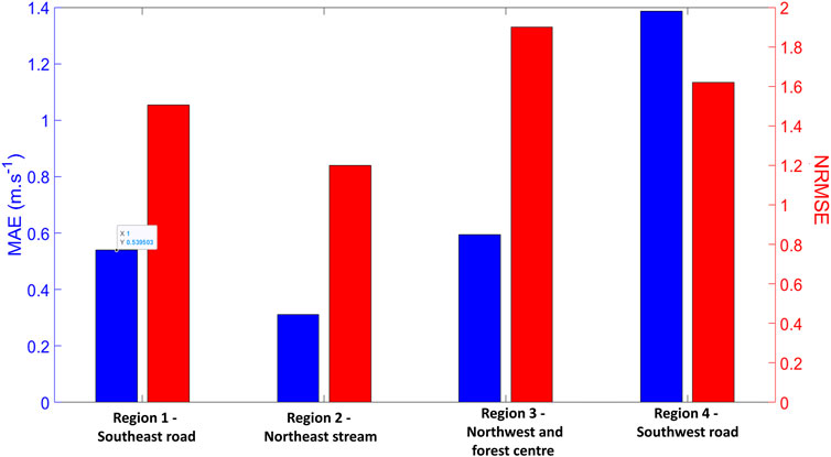
FIGURE 12. Similar to Figure 7. Here, the errors are averaged for the observations made over the four regions detailed in Section 3.2. They confirm that the best results were obtained in Region 2 and Region 1, as observed in Figure 5. For the first three regions, the relatively low MAE indicates that the model could perform reasonably well in a very complex canopy. High NRMSE values can be explained by the large range of values reached by the canopy wind speeds in domain regions with very different canopy cover, and the presence of outliers in the data that makes statistical results more difficult to interpret. Region 4 showed the worst results because the wind observations were more impacted by forest-edge effects and tree wakes, not modeled in the present study.

TABLE 4

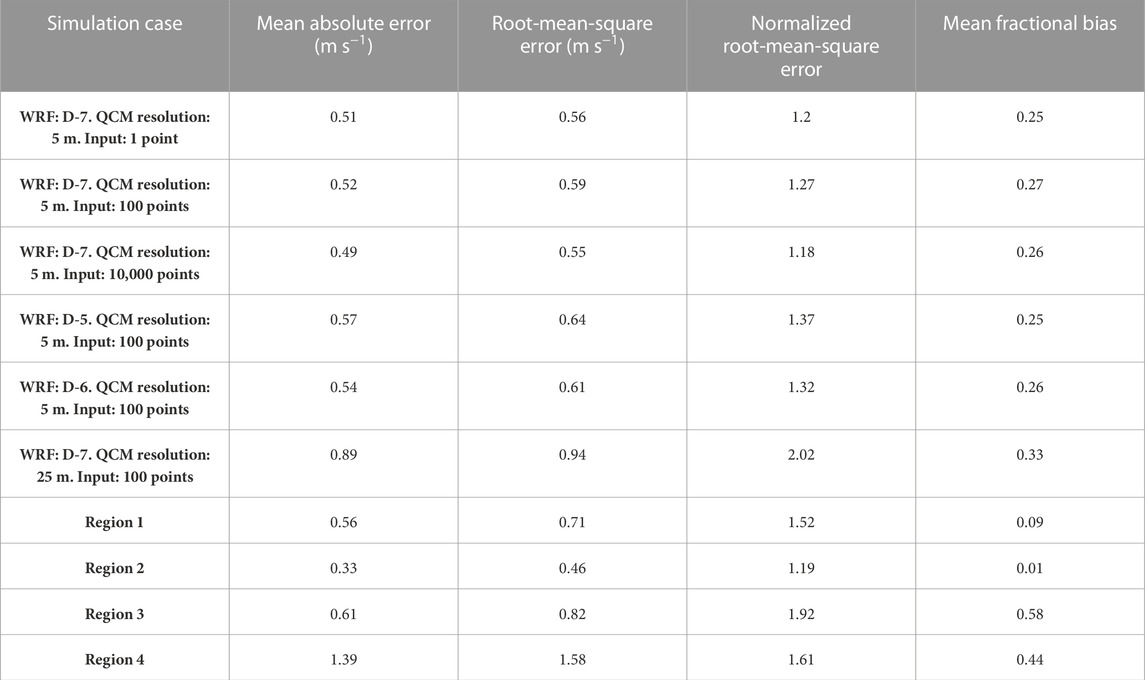
TABLE 4. The first six rows are error statistics for the six different numerical setups of the RxCADRE experiment described in Section 3.2.3. The third case is our reference configuration, and the last four rows present errors for the four regions shown in Fig. 5 with this reference setup. Simulation results were interpolated at the observation location and computed every minute during the 3 hours of the simulation.

5 Summary and conclusion

In this paper, we implemented a new mathematical framework for canopy winds in the fast response model QUIC and examined the frameworks performance in predicting high-resolution wind fields in heterogeneous forested environments. The new canopy wind model, QCM, takes advantage of the increasing availability of high-resolution LiDAR data for plant canopies, and is particularly useful for situations with limited data, time, and computational power. The approach was compared against QUIC’s original model, based on the work of Cionco (1965), and a more recent model (Massman et al., 2017), using experimental data from a horizontally homogeneous orchard surveyed with a high-resolution observation tower (Patton et al., 2011), and a set of 31 ground-based anemometers in a large heterogeneous pine forest (Ottmar et al., 2016a). In the latter case, QUIC was coupled with the large-scale prognostic model WRF for simulation results at different resolutions.

Uniquely, the QCM solves for the non-local transfer of momentum within the canopy layer, and does not rely on empirical coefficients to model the canopy elements. It accurately depicts the average canopy wind profile features, i.e., wind unaffected above two to three times the effective canopy height, logarithmic wind profile above the canopy, abrupt wind attenuation below the canopy top logarithmically proportional to the vegetation density, and the formation of a sub-canopy jet. Of the tested models, only QCM could reproduce the SCJ feature due to its use of the canopy wind sub-model inspired by Zeng and Takahashi (2000) while using one less empirical coefficient than the original version. The QCM outperformed the other models when applied to predict the CHATS data over two different seasons and for all observed atmospheric stability conditions, which was largely due to its ability to predict the secondary wind maximum commonly observed in the CHATS orchard. In the RxCADRE forest case, we demonstrated that decreasing WRF simulation resolution (tens of meters to kilometers) or the number of points to initialize the QCM wind field (tens to tens of thousands of points), was not a critical factor in obtaining the best results (at least for the RxCADRE case). It was expected that the WRF horizontal resolution would not significantly affect the results because the simulations used a one-dimensional PBL scheme, as explained earlier (Section 3.2.2). The wind was more accurately computed in denser parts of the forest, where the momentum was mostly transferred vertically from winds above the canopy rather than advected horizontally through the forest, and ideally far from edges’ effects, as assumed by the hypothesis made to derive the model.

Fast-modeling applications are vast and cover many different types of research fields. As introduced in Figure 2, improved modeled wind fields in canopies can readily be applied to fire or disease spread modeling to promote better health conditions and preserve cities and natural resources. Moreover, since the model relies on few user-defined coefficients and can run on personal computers in a reasonable time (a few minutes for hours of physical simulation time), it is accessible to non-expert users. The version of QUIC presented in this study was only parallelized with Open Multi-Processing (OMP) routines, but a more advanced and faster version, called QES-Winds, that utilizes GPU-based parallelization has already been developed by Bozorgmehr et al. (2021). The new QUIC canopy wind model naturally integrates into the new code framework as well as other similar frameworks, such as WindNinja (Forthofer et al., 2014).

An important limitation of the current model is its potential inaccuracy on steep slopes, where downslope and upslope flows interact with the canopy flow in a complex manner (Finnigan et al., 2020). To address this issue, including a model for slope with vegetation would provide value for all applications taking place in regions with forested mountains, hills, canyons, etc. A second critical point to address is the definition of a clear threshold for the resolution at which it is best to represent the vegetation as a collection of single elements, or a patch of constant averaged density. In other words, we need to quantify how homogeneous a vegetation patch must be to allow the application of volume-averaging operators, an essential transformation in the canopy wind modeling framework. This question is now made relevant thanks to the increased availability of high-resolution LiDAR instruments or satellite data, and its answer will help to address the ever-growing need to model how forest heterogeneity impacts wildfire rate of spread (as studied by Moody et al., 2023) or the wind velocity field, as examined in the present article. Finally, it would be interesting to simulate the wind field in vegetated areas in urban environments, like large parks in cities or nearby forests. Indeed, these locations play a great role in the control of temperature and humidity variations, as well as the attenuation or blocking of particles like pollutants.

Data availability statement

Publicly available datasets were analyzed in this study. This data can be found here: https://data.eol.ucar.edu/project/CHATS, https://data.nal.usda.gov, https://www.firelab.org/project/rxcadre-project.

Author contributions

MR contributed to model development, experimental validation, errors analysis, and writing of the document. EP and RS contributed to data collection, project advising, research study design, results interpretation, and review of the document. BB contributed to providing high-resolution LAD and LAI datasets for the CHATS experiment, and editing of the document. All authors contributed to the article and approved the submitted version.

Funding

This research was supported by the National Science Foundation under grant PREEVENTS 1664175.

Acknowledgments

The authors would like to thank Dr. Adam Kochanski and Dr. Derek V. Mallia for sharing the WRF simulations results for the RxCADRE case.

Conflict of interest

The authors declare that the research was conducted in the absence of any commercial or financial relationships that could be construed as a potential conflict of interest.

Publisher’s note

All claims expressed in this article are solely those of the authors and do not necessarily represent those of their affiliated organizations, or those of the publisher, the editors and the reviewers. Any product that may be evaluated in this article, or claim that may be made by its manufacturer, is not guaranteed or endorsed by the publisher.

Supplementary material

The Supplementary Material for this article can be found online at: https://www.frontiersin.org/articles/10.3389/feart.2023.1251056/full#supplementary-material

References

Albini, F. (1981). A phenomenological model for wind speed and shear stress profiles in vegetation cover layers. J. Appl. Meteorology 20, 1325–1335. doi:10.1175/1520-0450(1981)020<1325:apmfws>2.0.co;2

CrossRef Full Text | Google Scholar

Amorim, J., Rodrigues, V., Tavares, R., Valente, J., and Borrego, C. (2013). Cfd modelling of the aerodynamic effect of trees on urban air pollution dispersion. Sci. Total Environ. 461, 541–551. doi:10.1016/j.scitotenv.2013.05.031

PubMed Abstract | CrossRef Full Text | Google Scholar

Anjewierden, C. (2020). Enabling of the Quick urban industrial complex wind model to represent wind turbine flows. UT, United States: University of Utah.

Google Scholar

Arthur, R. S., Mirocha, J. D., Lundquist, K. A., and Street, R. L. (2019). Using a canopy model framework to improve large-eddy simulations of the neutral atmospheric boundary layer in the weather research and forecasting model. Mon. Weather Rev. 147, 31–52. doi:10.1175/MWR-D-18-0204.1

CrossRef Full Text | Google Scholar

Arya, P. S. (2001). Introduction to micrometeorology. Elsevier.

Google Scholar

Bailey, B. N., and Stoll, R. (2016). The creation and evolution of coherent structures in plant canopy flows and their role in turbulent transport. J. Fluid Mech. 789, 425–460. doi:10.1017/jfm.2015.749

CrossRef Full Text | Google Scholar

Barnes, S. L. (1973). Mesoscale objective map analysis using weighted time-series observations. Norman, OK: National Severe Storms Laboratory. doi:10.4135/9781544377230.n58

CrossRef Full Text | Google Scholar

Beaucage, P., Brower, M. C., and Tensen, J. (2012). Evaluation of four numerical wind flow models for wind resource mapping. Wind Energy 17 (2), 197–208. doi:10.1002/we.1568

CrossRef Full Text | Google Scholar

Boussinesq, J. (1877). Essai sur la theorie des eaux courantes. Imprimerie Nationale.

Google Scholar

Bozorgmehr, B., Willemsen, P., Gibbs, J. A., Stoll, R., Kim, J. J., and Pardyjak, E. R. (2021). Utilizing dynamic parallelism in CUDA to accelerate a 3d red-black successive over relaxation wind-field solver. Environ. Model. Softw. 137, 104958. doi:10.1016/j.envsoft.2021.104958

CrossRef Full Text | Google Scholar

Brown, B. J., Shapkalijevski, M., Krol, M., Karl, T., Ouwersloot, H., Moene, A., et al. (2020). Ozone exchange within and above an irrigated californian orchard. Tellus B Chem. Phys. Meteorology 72 (1), 1723346–1723417. doi:10.1080/16000889.2020.1723346

CrossRef Full Text | Google Scholar

Brown, M., Gowardhan, A., Nelson, M., Williams, M., and Pardyjak, E. (2013). QUIC transport and dispersion modelling of two releases from the joint urban 2003 field experiment. Int. J. Environ. Pollut. 52, 263–287. doi:10.1504/ijep.2013.058458

CrossRef Full Text | Google Scholar

Brunet, Y. (2020). Turbulent flow in plant canopies: historical perspective and overview, 177. Springer Netherlands, 315–364. doi:10.1007/s10546-020-00560-7

CrossRef Full Text | Google Scholar

Businger, J., Wyngaard, J., Izumi, Y., and Bradley, E. (1971). Flux-profile relationships in the atmospheric surface layer. J. Atmos. Sci. 28, 181–189. doi:10.1175/1520-0469(1971)028⟨0181:FPRITA⟩2.0.CO;2

CrossRef Full Text | Google Scholar

Cionco, R., Aufm Kampe, W., Biltoft, C., Byers, J., Collins, C., Higgs, T., et al. (1999). An overview of MADONA: a multinational field study of high-resolution meteorology and diffusion over complex terrain. Bull. Am. Meteorological Soc. 80 (1), 5–19. doi:10.1175/1520-0477(1999)080<0005:aoomam>2.0.co;2

CrossRef Full Text | Google Scholar

Cionco, R. M. (1965). A mathematical model for air flow in a vegetative canopy. J. Appl. Meteorology Climatol. 4 (4), 517–522. doi:10.1175/1520-0450(1965)004<0517:ammfaf>2.0.co;2

CrossRef Full Text | Google Scholar

Cionco, R. M. (1972). A wind-profile index for canopy flow. Boundary-Layer Meteorol. 3 (2), 255–263. doi:10.1007/BF02033923

CrossRef Full Text | Google Scholar

Coceal, O., and Belcher, S. E. (2004). A canopy model of mean winds through urban areas. Q. J. R. Meteorological Soc. 130, 1349–1372. doi:10.1256/qj.03.40

CrossRef Full Text | Google Scholar

Delle Monache, L., Weil, J., Simpson, M., and Leach, M. (2009). A new urban boundary layer and dispersion parameterization for an emergency response modeling system: tests with the joint urban 2003 data set. Atmos. Environ. 43, 5807–5821. doi:10.1016/j.atmosenv.2009.07.051

CrossRef Full Text | Google Scholar

Dupont, S., and Patton, E. G. (2012). Influence of stability and seasonal canopy changes on micrometeorology within and above an orchard canopy: the chats experiment. Agric. For. Meteorology 157, 11–29. doi:10.1016/j.agrformet.2012.01.011

CrossRef Full Text | Google Scholar

Finnigan, J. J., Ayotte, K. W., Harman, I. N., Katul, G. G., Oldroyd, H. J., Patton, E. G., et al. (2020). Boundary-layer flow over complex topography. Boundary-Layer Meteorol. 177 (2–4), 247–313. doi:10.1007/s10546-020-00564-3

CrossRef Full Text | Google Scholar

Forthofer, J. M., Butler, B. W., and Wagenbrenner, N. S. (2014). A comparison of three approaches for simulating fine-scale surface winds in support of wildland fire management. Part I. Model formulation and comparison against measurements. Int. J. Wildland Fire 23 (7), 969–981. doi:10.1071/WF12089

CrossRef Full Text | Google Scholar

Garratt, J. R. O. (1992). The atmospheric boundary layer. Cambridge University Press.

Google Scholar

Girard, P., Nadeau, D. F., Pardyjak, E. R., Overby, M. C., Willemsen, P., Stoll, R., et al. (2018). Evaluation of the QUIC-URB wind solver and QESRadiant radiation-transfer model using a dense array of urban meteorological observations. Urban Clim. 24, 657–674. doi:10.1016/j.uclim.2017.08.006

CrossRef Full Text | Google Scholar

Golzio, A., Ferrarese, S., Cassardo, C., Diolaiuti, G. A., and Pelfini, M. (2021). Land-use improvements in the weather research and forecasting model over complex mountainous terrain and comparison of different grid sizes. Boundary-Layer Meteorol. 180 (2), 319–351. doi:10.1007/s10546-021-00617-1

CrossRef Full Text | Google Scholar

Grant, E. R., Ross, A. N., Gardiner, B. A., and Mobbs, S. D. (2015). Field observations of canopy flows over complex terrain. Boundary-Layer Meteorol. 156, 231–251. doi:10.1007/s10546-015-0015-y

CrossRef Full Text | Google Scholar

Grimmond, C. S. B., and Oke, T. R. (1999). Aerodynamic properties of urban areas derived from analysis of surface form. J. Appl. Meteorology 38 (9), 1262–1292. doi:10.1175/1520-0450(1999)038⟨1262:APOUAD⟩2.0.CO;2

CrossRef Full Text | Google Scholar

Guan, D., Agarwal, P., and Chiew, Y.-M. (2018). Quadrant analysis of turbulence in a rectangular cavity with large aspect ratios. J. Hydraulic Eng. 144 (7), 04018035. doi:10.1061/(asce)hy.1943-7900.0001480

CrossRef Full Text | Google Scholar

Halubok, M., Kochanski, A. K., Stoll, R., and Bailey, B. N. (2021). Errors in the estimation of leaf area density from aerial lidar data: influence of statistical sampling and heterogeneity. IEEE Trans. Geoscience Remote Sens. 60, 1–14. doi:10.1109/tgrs.2021.3123585

CrossRef Full Text | Google Scholar

Harman, I. N., and Finnigan, J. J. (2007). A simple unified theory for flow in the canopy and roughness sublayer. Boundary-Layer Meteorol. 123 (2), 339–363. doi:10.1007/s10546-006-9145-6

CrossRef Full Text | Google Scholar

Hayati, A. N., Stoll, R., Kim, J. J., Harman, T., Nelson, M. A., Brown, M. J., et al. (2017). Comprehensive evaluation of fast-response, Reynolds-averaged Navier–Stokes, and large-eddy simulation methods against high-spatial-resolution wind-tunnel data in step-down street canyons. Boundary-Layer Meteorol. 164, 217–247. doi:10.1007/s10546-017-0245-2

CrossRef Full Text | Google Scholar

Hayati, A. N., Stoll, R., Pardyjak, E. R., Harman, T., and Kim, J. (2019). Comparative metrics for computational approaches in non-uniform street-canyon flows. Build. Environ. 158, 16–27. doi:10.1016/j.buildenv.2019.04.028

CrossRef Full Text | Google Scholar

Hertwig, D., Soulhac, L., Fuka, V., Auerswald, T., Carpentieri, M., Hayden, P., et al. (2018). Evaluation of fast atmospheric dispersion models in a regular street network. Environ. Fluid Mech. 18, 1007–1044. doi:10.1007/s10652-018-9587-7

CrossRef Full Text | Google Scholar

Hoffman, C. M., Linn, R., Parsons, R., Sieg, C., and Winterkamp, J. (2015). Modeling spatial and temporal dynamics of wind flow and potential fire behavior following a mountain pine beetle outbreak in a lodgepole pine forest. Agric. For. Meteorology 204, 79–93. doi:10.1016/j.agrformet.2015.01.018

CrossRef Full Text | Google Scholar

Hong, S.-Y., Noh, Y., and Dudhia, J. (2006). A new vertical diffusion package with an explicit treatment of entrainment processes. Mon. Weather Rev. 134, 2318–2341. doi:10.1175/MWR3199.1

CrossRef Full Text | Google Scholar

Katul, G. G., Mahrt, L., Poggi, D., and Sanz, C. (2004). One-and two-equation models for canopy turbulence. Boundary-layer Meteorol. 113, 81–109. doi:10.1023/b:boun.0000037333.48760.e5

CrossRef Full Text | Google Scholar

Koch, S. E., DesJardins, M., and Kocin, P. J. (1983). An interactive barnes objective map analysis scheme for use with satellite and conventional data. J. Appl. Meteorology Climatol. 22 (9), 1487–1503. doi:10.1175/1520-0450(1983)022<1487:aiboma>2.0.co;2

CrossRef Full Text | Google Scholar

Kochanski, A. K., Pardyjak, E. R., Stoll, R., Gowardhan, A. A., Brown, M. J., and Steenburgh, W. J. (2015). One-way coupling of the WRF-QUIC Urban dispersion modeling system. J. Appl. Meteorology Climatol. 54 (10), 2119–2139. doi:10.1175/JAMC-D-15-0020.1

CrossRef Full Text | Google Scholar

Kondo, J., and Akashi, S. (1976). Numerical studies on the two-dimensional flow in horizontally homogeneous canopy layers. Boundary-Layer Meteorol. 10, 255–272. doi:10.1007/bf00919389

CrossRef Full Text | Google Scholar

Li, Z. J., Miller, D. R., and Lim, J. D. (1985). A first-order closure scheme to describe counter-gradient momentum transport in plant canopies. Boundary-Layer Meteorol. 33, 77–83. doi:10.1007/bf00137037

CrossRef Full Text | Google Scholar

Linn, R. R., Goodrick, S. L., Brambilla, S., Brown, M. J., Middleton, R. S., and O'Brien, J. J. (2020). QUIC-fire: a fast-running simulation tool for prescribed fire planning. Environ. Model Softw. 125, 104616. doi:10.1016/j.envsoft.2019.104616

CrossRef Full Text | Google Scholar

Liu, Y., Li, H., Sun, S., and Fang, S. (2017). Enhanced air dispersion modelling at a typical Chinese nuclear power plant site: coupling rimpuff with two advanced diagnostic wind models. J. Environ. Radioact. 175-176, 94–104. doi:10.1016/j.jenvrad.2017.04.016

PubMed Abstract | CrossRef Full Text | Google Scholar

Ludwig, F. L., Miller, D. K., and Gallaher, S. G. (2006). Evaluating a hybrid prognostic–diagnostic model that improves wind forecast resolution in complex coastal topography. J. Appl. Meteorology Climatol. 45, 155–177. doi:10.1175/JAM2329.1

CrossRef Full Text | Google Scholar

Ma, Y., and Liu, H. (2019). An advanced multiple-layer canopy model in the wrf model with large-eddy simulations to simulate canopy flows and scalar transport under different stability conditions. J. Adv. Model. Earth Syst. 11, 2330–2351. doi:10.1029/2018MS001347

CrossRef Full Text | Google Scholar

Ma, Y., Liu, H., Banerjee, T., Katul, G. G., Yi, C., and Pardyjak, E. R. (2020). The effects of canopy morphology on flow over a two-dimensional isolated ridge. J. Geophys. Res. Atmos. 125 (19), e2020JD033027. doi:10.1029/2020jd033027

CrossRef Full Text | Google Scholar

Macdonald, R. W. (2000). Modelling the mean velocity profile in the urban canopy layer. Boundary-Layer Meteorol. 97 (1), 25–45. doi:10.1023/A:1002785830512

CrossRef Full Text | Google Scholar

Mahaffee, W. F., Margairaz, F., Ulmer, L., Bailey, B. N., and Stoll, R. (2023). Catching spores: linking epidemiology, pathogen biology, and physics to ground-based airborne inoculum monitoring. Plant Dis. 107 (1), 13–33. doi:10.1094/pdis-11-21-2570-fe

PubMed Abstract | CrossRef Full Text | Google Scholar

Mallia, D. V., Kochanski, A. K., Urbanski, S. P., Mandel, J., Farguell, A., and Krueger, S. K. (2020). Incorporating a canopy parameterization within a coupled fire-atmosphere model to improve a smoke simulation for a prescribed burn. Atmosphere 11 (8), 832. doi:10.3390/ATMOS11080832

CrossRef Full Text | Google Scholar

Mandel, J., Beezley, J. D., and Kochanski, A. K. (2011). Coupled atmosphere-wildland fire modeling with WRF 3.3 and SFIRE 2011. Geosci. Model Dev. 4, 591–610. doi:10.5194/gmd-4-591-2011

CrossRef Full Text | Google Scholar

Margairaz, F., Eshagh, H., Hayati, A. N., Pardyjak, E. R., and Stoll, R. (2022). Development and evaluation of an isolated-tree flow model for neutral-stability conditions. Urban Clim. 42, 101083. doi:10.1016/j.uclim.2022.101083

CrossRef Full Text | Google Scholar

Massman, W. (1997). An analytical one-dimensional model of momentum transfer by vegetation of arbitrary structure. Boundary-Layer Meteorol. 83, 407–421. doi:10.1023/a:1000234813011

CrossRef Full Text | Google Scholar

Massman, W. J., Forthofer, J. M., and Finney, M. A. (2017). An improved canopy wind model for predicting wind adjustment factors and wildland fire behavior. Can. J. For. Res. 47 (5), 594–603. doi:10.1139/cjfr-2016-0354

CrossRef Full Text | Google Scholar

Miller, D., Lin, J., and Lu, Z. (1991). Air flow across an alpine forest clearing: a model and field measurements. Agric. For. Meteorology 56 (3), 209–225. doi:10.1016/0168-1923(91)90092-5

CrossRef Full Text | Google Scholar

Moin, P., and Mahesh, K. (1998). Direct numerical simulation: a tool in turbulence research. Annu. Rev. fluid Mech. 30, 539–578. doi:10.1146/annurev.fluid.30.1.539

CrossRef Full Text | Google Scholar

Monin, A. S., and Obukhov, A. M. (1954). Basic laws of turbulent mixing in the surface layer of the atmosphere. Contrib. Geophys. Inst. Acad. Sci. USSR 24 (151), 163–187.

Google Scholar

Moody, M. J., Gibbs, J. A., Krueger, S., Mallia, D., Pardyjak, E. R., Kochanski, A. K., et al. (2022). QES-fire: a dynamically coupled fast-response wildfire model. Int. J. Wildland Fire 31 (3), 306–325. doi:10.1071/WF21057

CrossRef Full Text | Google Scholar

Moody, M. J., Stoll, R., and Bailey, B. N. (2023). Adaptation of QES-Fire, a dynamically coupled fast response wildfire model for heterogeneous environments. Int. J. Wildland Fire 32, 749–766. doi:10.1071/wf22190

CrossRef Full Text | Google Scholar

Nathan, R., Katul, G. G., Horn, H. S., Thomas, S. M., Oren, R., Avissar, R., et al. (2002). Mechanisms of long-distance dispersal of seeds by wind. Nature 418 (6896), 409–413. doi:10.1038/nature00844

PubMed Abstract | CrossRef Full Text | Google Scholar

Neophytou, M., Gowardhan, A., and Brown, M. (2011). An inter-comparison of three urban wind models using Oklahoma city joint urban 2003 wind field measurements. J. Wind Eng. Industrial Aerodynamics 99 (4), 357–368. doi:10.1016/j.jweia.2011.01.010

CrossRef Full Text | Google Scholar

Nieto, H., Kustas, W. P., Alfieri, J. G., Gao, F., Hipps, L. E., Los, S., et al. (2019). Impact of different within-canopy wind attenuation formulations on modelling sensible heat flux using tseb. Irrigation Sci. 37, 315–331. doi:10.1007/s00271-018-0611-y

CrossRef Full Text | Google Scholar

Niu, G.-Y., Yang, Z.-L., Mitchell, K. E., Chen, F., Ek, M. B., Barlage, M., et al. (2011). The community Noah land surface model with multiparameterization options (Noah-MP): 1. Model description and evaluation with local-scale measurements. J. Geophys. Res. Atmos. 116, D12109. doi:10.1029/2010jd015139

CrossRef Full Text | Google Scholar

Oldroyd, H. J., Katul, G., Pardyjak, E. R., and Parlange, M. B. (2014). Momentum balance of katabatic flow on steep slopes covered with short vegetation. Geophys. Res. Lett. 41, 4761–4768. doi:10.1002/2014gl060313

CrossRef Full Text | Google Scholar

Ottmar, R. D., Hiers, J. K., Butler, B. W., Clements, C. B., Dickinson, M. B., Hudak, A. T., et al. (2016a). Measurements, datasets and preliminary results from the RxCADRE project - 2008, 2011 and 2012. Int. J. Wildland Fire 25 (1), 1–9. doi:10.1071/WF14161

CrossRef Full Text | Google Scholar

Ottmar, R. D., Hudak, A. T., Prichard, S. J., Wright, C. S., Restaino, J. C., Kennedy, M. C., et al. (2016b). Pre-fire and post-fire surface fuel and cover measurements collected in the south-eastern United States for model evaluation and development – RxCADRE 2008, 2011 and 2012. Int. J. Wildland Fire 25 (1), 10–24. doi:10.1071/WF15092

CrossRef Full Text | Google Scholar

Pan, Y., and Patton, E. G. (2020). Determining stationary periods across multiple sensors: an application to observed canopy turbulence response to atmospheric stability. J. Atmos. Ocean. Technol. 37 (4), 665–685. doi:10.1175/jtech-d-19-0135.1

CrossRef Full Text | Google Scholar

Pardyjak, E. R., and Brown, M. (2003). QUIC-URB v. 1.1: theory and user’s guide. Los Alamos, NM: Los Alamos National Laboratory.

Google Scholar

Pardyjak, E. R., Speckart, S. O., Yin, F., and Veranth, J. M. (2008). Near source deposition of vehicle generated fugitive dust on vegetation and buildings: model development and theory. Atmos. Environ. 42 (26), 6442–6452. doi:10.1016/j.atmosenv.2008.04.024

CrossRef Full Text | Google Scholar

Patton, E. G., Horst, T. W., Sullivan, P. P., Lenschow, D. H., Oncley, S. P., Brown, W. O. J., et al. (2011). The canopy horizontal array turbulence study. Bull. Am. Meteorological Soc. 92 (5), 593–611. doi:10.1175/2010BAMS2614.1

CrossRef Full Text | Google Scholar

Piomelli, U. (1999). Large-eddy simulation: achievements and challenges. Prog. Aerosp. Sci. 35, 335–362. doi:10.1016/s0376-0421(98)00014-1

CrossRef Full Text | Google Scholar

Pol, S., Bagal, N., Singh, B., Brown, M., and Pardyjak, E. (2006). “Implementation of a new rooftop recirculation parameterization into the QUIC fast-response urban wind model,” in 86th AMS annual meeting. JP1.2.

Google Scholar

Porté-Agel, F., Bastankhah, M., and Shamsoddin, S. (2020). Wind-turbine and wind-farm flows: a review. Boundary-layer Meteorol. 174, 1–59. doi:10.1007/s10546-019-00473-0

PubMed Abstract | CrossRef Full Text | Google Scholar

Prandtl, L. (1932). Meteorogische an wendung der stromungslehre. Beitr. Phys. At. 19.

Google Scholar

Ratto, C. F., Festa, R., Romeo, C., Frumento, O. A., and Galluzzi, M. (1994). Mass-consistent models for wind fields over complex terrain: the state of the art. Environ. Softw. 9 (5), 247–268. doi:10.1016/0266-9838(94)90023-X

CrossRef Full Text | Google Scholar

Raupach, M. R. (1994). Simplified expressions for vegetation roughness length and zero-plane displacement as functions of canopy height and area index. Boundary-Layer Meteorol. 71 (1–2), 211–216. doi:10.1007/BF00709229

CrossRef Full Text | Google Scholar

Raupach, M. R., Coppin, P. A., and Legg, B. J. (1986). Experiments on scalar dispersion within a model plant canopy part i: the turbulence structure. Boundary-Layer Meteorol. 35, 21–52. doi:10.1007/BF00117300

CrossRef Full Text | Google Scholar

Raupach, M. R., Finnigan, J. J., and Brunet, Y. (1996). Coherent eddies and turbulence in vegetation canopies: the mixing-layer analogy. Boundary-Layer Meteorol. 78 (3–4), 351–382. doi:10.1007/BF00120941

CrossRef Full Text | Google Scholar

Raupach, M. R., and Shaw, R. H. (1982). Averaging procedures for flow within vegetation canopies. Boundary-Layer Meteorol. 22 (1), 79–90. doi:10.1007/BF00128057

CrossRef Full Text | Google Scholar

Sasaki, Y. (1970). Some basic formalisms in numerical variational analysis. Mon. Weather Rev. 98 (12), 875–883. doi:10.1175/1520-0493(1970)098⟨0875:sbfinv⟩2.3.co;2

CrossRef Full Text | Google Scholar

Schmid, M. F., Lawrence, G. A., Parlange, M. B., and Giometto, M. G. (2019). Volume averaging for urban canopies. Boundary-Layer Meteorol. 173 (3), 349–372. doi:10.1007/s10546-019-00470-3

PubMed Abstract | CrossRef Full Text | Google Scholar

Segalini, A., Nakamura, T., and Fukagata, K. (2016). A linearized k - ϵ model of forest canopies and clearings. Boundary-Layer Meteorol. 161 (3), 439–460. doi:10.1007/s10546-016-0190-5

CrossRef Full Text | Google Scholar

Sharma, A., and García-Mayoral, R. (2020). Turbulent flows over dense filament canopies. J. Fluid Mech. 888 (A2), 1–38. doi:10.1017/jfm.2020.27

CrossRef Full Text | Google Scholar

Shaw, R. (1977). Secondary wind speed maxima inside plant canopies. J. Appl. Meteorology 16, 514–521. doi:10.1175/1520-0450(1977)016⟨0514:SWSMIP⟩2.0.CO;2

CrossRef Full Text | Google Scholar

Shaw, R. H., and Pereira, A. (1982). Aerodynamic roughness of a plant canopy: a numerical experiment. Agric. Meteorol. 26 (1), 51–65. doi:10.1016/0002-1571(82)90057-7

CrossRef Full Text | Google Scholar

Sherman, C. A. (1978). A mass consistent model for wind fields over complex terrain. J. Appl. Meteorology 17, 312–319. doi:10.1175/1520-0450(1978)017<0312:amcmfw>2.0.co;2

CrossRef Full Text | Google Scholar

Silva, J., Ribeiro, C., and Guedes, R. (2007). “Roughness length classification of corine land cover classes,” in Proceedings of the European wind energy conference (Milan, Italy: Citeseer), 710, 110.

Google Scholar

Skamarock, W. C., Klemp, J. B., Dudhia, J. B., Gill, D. O., Barker, D. M., Duda, M. G., et al. (2008). A description of the advanced research WRF version 3, NCAR technical note TN-475+STR. Technical Report, 113.

Google Scholar

Speckart, S. O., and Pardyjak, E. R. (2014). A method for rapidly computing windbreak flow field variables. J. Wind Eng. Industrial Aerodynamics 132, 101–108. doi:10.1016/j.jweia.2014.07.001

CrossRef Full Text | Google Scholar

Stoll, R., Gibbs, J. A., Salesky, S. T., Anderson, W., and Calaf, M. (2020). Large-eddy simulation of the atmospheric boundary layer. Boundary-Layer Meteorol. 177, 541–581. doi:10.1007/s10546-020-00556-3

CrossRef Full Text | Google Scholar

Stull, R. B. (1988). An introduction to boundary layer meteorology, 13. Springer Science and Business Media.

Google Scholar

Su, H.-B., Schmid, H., Vogel, C., and Curtis, P. (2008). Effects of canopy morphology and thermal stability on mean flow and turbulence statistics observed inside a mixed hardwood forest. Agric. For. Meteorology 148 (6), 862–882. doi:10.1016/j.agrformet.2007.12.002

CrossRef Full Text | Google Scholar

Sypka, P., and Starzak, R. (2012). Simplified, empirical model of wind speed profile under canopy of istebna spruce stand in mountain valley. Agric. For. Meteorology 171-172, 220–233. doi:10.1016/j.agrformet.2012.11.003

CrossRef Full Text | Google Scholar

Thomas, C., Mayer, J.-C., Meixner, F. X., and Foken, T. (2006). Analysis of low-frequency turbulence above tall vegetation using a Doppler sodar. Boundary-Layer Meteorol. 119 (3), 563–587. doi:10.1007/s10546-005-9038-0

CrossRef Full Text | Google Scholar

Uchijima, Z. (1962). Studies on the micro-climate within the plant communities. J. Agric. Meteorology 18 (1), 1–9. doi:10.2480/agrmet.18.1

CrossRef Full Text | Google Scholar

Ulmer, L., Margairaz, F., Bailey, B. N., Mahaffee, W. F., Pardyjak, E. R., and Stoll, R. (2023). A fast-response, wind angle-sensitive model for predicting mean winds in row-organized canopies. Agric. For. Meteorology 329, 109273. doi:10.1016/j.agrformet.2022.109273

CrossRef Full Text | Google Scholar

Wang, W., Shaw, W. J., Seiple, T. E., Rishel, J. P., and Xie, Y. (2008). An evaluation of a diagnostic wind model (calmet). J. Appl. Meteorology Climatol. 47, 1739–1756. doi:10.1175/2007JAMC1602.1

CrossRef Full Text | Google Scholar

Weickert, J., Romeny, B. T. H., and Viergever, M. A. (1998). Efficient and reliable schemes for nonlinear diffusion filtering. IEEE Trans. image Process. 7 (3), 398–410. doi:10.1109/83.661190

PubMed Abstract | CrossRef Full Text | Google Scholar

Williams, M. D., Brown, M. J., Boswell, D., Singh, B., and Pardyjak, E. M. (2004). “Testing of the QUIC-plume model with wind-tunnel measurements for a high-rise building,” in 5th AMS symposium meeting (United States) (Los Alamos, NM, United States), J5.3. Research org.: los alamos national lab. (LANL).

Google Scholar

Wilson, J. D., Swaters, G., and Ustine, F. (1990). A perturbation analysis of turbulent flow through a porous barrier. Q. J. R. Meteorological Soc. 116 (494), 989–1004. doi:10.1002/qj.49711649410

CrossRef Full Text | Google Scholar

Zeng, P., and Takahashi, H. (2000). A first-order closure model for the wind flow within and above vegetation canopies. Agric. For. Meteorology 103 (3), 301–313. doi:10.1016/S0168-1923(00)00133-7

CrossRef Full Text | Google Scholar