Advancing very short-term rainfall prediction with blended U-Net and partial differential approaches

Accurate and timely prediction of short-term rainfall is crucial for reducing the damages caused by heavy rainfall events. Therefore, various precipitation nowcasting models have been proposed. However, the performance of these models still remains limited. In particular, the current operational precipitation nowcasting method, which is based on radar echo tracking, such as the McGill Algorithm for Precipitation Nowcasting by Lagrangian Extrapolation (MAPLE), has a critical drawback when predicting newly developed or decayed precipitation fields. Recently proposed deep learning models, such as the U-Net convolutional neural network outperform the models based on radar echo tracking. However, these models are unsuitable for operational precipitation nowcasting due to their blurry predictions over longer lead times. To address these blurry effects and enhance the performance of U-Net-based rainfall prediction, we propose a blended model that combines a partial differential equation (PDE) model based on fluid dynamics with the U-Net model. The evaluation of the forecast skill, based on both qualitative and quantitative methods for 0–3-h lead times, demonstrates that the blended model provides less blurry and more accurate rainfall predictions compared with the U-Net and partial differential equation models. This indicates the potential to enhance the field of very short-term rainfall prediction. Additionally, we also evaluated the monthly-averaged forecast skills for different seasons, and confirmed the operational feasibility of the blended model, which contributes to the performance enhancement of operational nowcasting.

1 Introduction

Accurate and timely predictions of short-term rainfall are crucial for minimizing damages caused by heavy rainfall events. These damages include economic and human losses owing to flooding, as well as disruptions in daily life, such as transportation, including air travel. For example, during the summer of 2020, South Korea experienced destructive floods, causing economic losses amounting to billions of dollars (KMA, 2021). To mitigate such damages, precise short-term rainfall predictions within 0–6-h lead times are necessary (e.g., Kox et al., 2015; Sivle et al., 2022).

Radar echo tracking methods utilizing weather radar data, such as the McGill Algorithm for Precipitation nowcasting by Lagrangian Extrapolation (MAPLE), have been employed in operational short-term rainfall prediction models (e.g., Germann and Zawadzki, 2002; Germann and Zawadzki, 2004; Turner et al., 2004; Germann et al., 2006; Lee et al., 2010), and Python open-source libraries for precipitation nowcasting based on such methods have been also proposed, such as rainymotion v1.0 (Ayzel et al., 2019) and PySTEPS (Pulkkinen et al., 2019). Additionally, more sophisticated models have been proposed by considering advection-diffusion equations and non-stationary velocity fields, and such models outperform MAPLE, which solely handles advection (Ryu et al., 2020). However, even with the ability of these models to predict the movement of precipitation patterns, limitations exist in their predictive performance owing to the difficulty in considering dynamical processes, such as precipitation generation and dissipation (e.g., Germann et al., 2006). In particular, a significant portion of rainfall exhibits a stationary front, thereby hindering rainfall prediction using the radar echo tracking methods.

Numerical weather prediction (NWP) models can forecast the dynamical processes, such as growth and decay of precipitation fields, by incorporating atmospheric physics (e.g., Benjamin et al., 2004; Shrestha et al., 2013; Sun et al., 2014; Wang et al., 2016; Yu et al., 2017). Compared with the radar echo tracking methods, NWP can model the dynamical processes, including the growth and decay of precipitation fields. However, their spin-up time has limitations in achieving accurate performance within lead times of a few hours (e.g., Sun et al., 2014).

Recently, deep learning-based models have been studied to predict the non-linear evolution of precipitation patterns (e.g., Shi et al., 2015; Shi et al., 2017; Agrawal et al., 2019; Lebedev et al., 2019; Ayzel et al., 2020; Sønderby et al., 2020; Ravuri et al., 2021; Kim and Hong, 2022a; Kim and Hong, 2022b; Choi and Kim, 2022; Ko et al., 2022; Oh et al., 2023). These models are data-driven and physics-free, as they can be trained using high-resolution radar data that contain spatiotemporal information on instantaneous rainfall. S-band radar has a spatiotemporal resolution of approximately 10-min intervals and 1-km scale (Thorndabl et al., 2017), enabling sufficiently high-resolution predictions within 0–6-h lead times. In particular, models based on convolutional long short-term memory (Conv-LSTM) and U-Net have previously been proposed, wherein multiple past radar images are used as input data to train the model and predict future timestep images (Shi et al., 2015; 2017; Agrawal et al., 2019; Lebedev et al., 2019; Ayzel et al., 2020; Sønderby et al., 2020; Kim and Hong, 2022a; Ko et al., 2022; Oh et al., 2023). These models learn the complex evolution of rainfall patterns over time, resulting in better predictive performance than baseline models, such as NWP, radar echo tracking, and Eulerian persistence. Such convolutional models, however, generate blurry prediction images with increasing prediction time; thus, adopting such models for operational precipitation nowcasting is unlikely. To resolve the issue of blurry images, Generative Adversarial Network (GAN)-based generative models have been proposed in previous studies to obtain predictions without blurry effects (e.g., Ravuri et al., 2021; Kim and Hong, 2022b; Choi and Kim, 2022). In particular, Ravuri et al. (2021) proposed a novel idea to produce spatiotemporally consistent prediction by employing spatial and temporal discriminators, which discourage blurry and temporally inconsistent predictions, respectively. Nevertheless, these predictive performances are not sustained over long periods (i.e., the prediction timescale is currently limited to around 0–2-h lead times) and exhibit decreased accuracy in predicting heavy rainfall events (e.g., Choi and Kim, 2022).

Studies have been conducted to improve the performance of convolutional models, such as U-Net. Various types of loss functions have been applied, leading to significant performance improvements (e.g., Bakkay et al., 2022). For instance, the utilization of the logcosh loss has positively impacted the predictive performance compared with that of simple MSE loss (Ayzel et al., 2020 and the references therein). In addition, some of recent studies have also employed the loss functions based on Critical Success Index (CSI), which is used to measure the agreement between predicted and observed precipitation (Chen et al., 2020; Ko et al., 2022). As demonstrated by Ko et al. (2022), the application of CSI-based loss is a substantial factor aiding in the development of a model that can outperform conventional convolutional models and generative models in terms of the rainfall forecasting accuracy. Along with the loss function, Ko et al. (2022) examined the dependence on the training method by employing pre-training and fine-tuning steps. According to their findings, the training method has a significant impact on improving the prediction accuracy. Furthermore, in recent studies, both radar and satellite data or surface observations have been used as training data for U-Net models. The incorporation of multiple observational data has shown promising results in improving model performance (e.g., Lebedev et al., 2019; Miao et al., 2020; Choi et al., 2021). These improvements suggest that if the blurry effects of U-Net models can be addressed, U-Net-based precipitation prediction models can be competitive.

In this study, we propose an approach to resolve the blurry predictions produced by U-Net-based model. Assuming that the evolution of precipitation patterns is primarily driven by certain processes, such as advection and temporal variations in rainfall intensity, U-Net-based models suffer from difficulties in tracking the advection of precipitation owing to blurry effects, whereas models based on the advection-diffusion equation struggle to predict the complex dynamical processes, such as the growth and/or decay of precipitation. To overcome these limitations, we first employed a model that utilizes detailed solutions of partial differential equations (PDEs) associated with fluid dynamics to capture the motion of precipitation fields. We then developed the model by combining the PDE-based and U-Net-based predictions, resulting in less blurry and more precise forecasts. The performance of the constructed blended model was quantitatively and qualitatively evaluated using precipitation cases on the Korean Peninsula. In particular, previous studies regarding the development of deep learning models for precipitation nowcasting have focused on constructing and evaluating deep learning models at the research level. However, in this study, we aim to propose practical approaches that maintain the prediction tendencies of PDE-based models already used in short-term operational forecasting, such as MAPLE, and enhance their performance by incorporating deep learning models into the current approaches of operational nowcasting. To explore the potential of this blended model for operational nowcasting, we also compared them with recently proposed deep learning-based models through baseline models, such as Eulerian persistence and U-Net.

The paper is organized as follows. Section 2 describes the dataset and model that were used in this study. Section 3 presents the performance of the model combining U-Net architecture and forecast based on PDEs. Section 4 provides a brief summary of the study.

2 Methods

2.1 Radar dataset

Korean Meteorological Administration (KMA) has provided radar data based on Hybrid Surface Rainfall (HSR) method since 2018. The HSR method is characterized by the synthesis of reflectivity at the hybrid surface that is unaffected by the ground clutter, beam blockage, non-meteorological echoes, and bright band (e.g., Kwon et al., 2015; Lyu et al., 2015; Lyu et al., 2017). The size of data is $2305\times 2880$ (or, $1152.5\text{\hspace{0.17em}km}\times 1440\text{\hspace{0.17em}km}$) and the spatial and temporal resolutions of the HSR data are 0.5 km and 5 min, respectively. From the radar reflectivity factor ($Z$), precipitation ($R$) can be estimated through the Z-R relationship of KMA, $R={\left(Z/148\right)}^{100/159}$.

For training the model described in Section 3, the HSR data from 2018, 2019, and 2021 were used and the prediction results were validated using the HSR data from 2020. We then tested and evaluated the performance of the model using the HSR data from 2022. The preprocessing step is summarized as follows: 1) $2\times 2$ max-pooling to reduce the spatial resolution of the original data from 0.5 km to 1km; 2) producing a cropped image with a final size of $1152\times 1152$; 3) applying the transformation, $R_{transformed}=\ln$ ($R_{raw}+0.01$), to address the data imbalance in precipitation; 4) Generating input data by stacking time-sequential images. When stacking, three images were used with a temporal resolution of 10 min.

The types of heavy rainfall events occurring in the Korean Peninsula and their characteristics have been extensively examined using self-organization map (SOM) and K-means clustering (Jo et al., 2020; Park et al., 2021). In previous studies, the classification of heavy rainfall events through the SOM method is explained based on the diverse synoptic weather patterns of the rainy season of Korea (i.e., typically from June to September), and a substantial fraction of such heavy rainfall events do not occur throughout the Korean Peninsula but rather in localized regions. Figure 1 shows two representative examples of heavy rainfall events typically occurring in South Korea. The first example shows a quasi-stationary monsoon front that occurred in the central region of the Korean Peninsula (Central case, hereafter). These types of rainfall typically occur due to a clash between the air masses around the Korean peninsula (e.g., Seo et al., 2015). The second example shows the heavy rainfall in the southern coastal area of Korean peninsula (Southern case, hereafter). Owing to the presence of a southwesterly low-level jet, which contains a large amount of moisture, such precipitation events are typically induced (e.g., Lee et al., 2008).

FIGURE 1

FIGURE 1. The rate of rain ($\text{mm\hspace{0.17em}}{\mathrm{h}}^{-1}$) of two precipitation events ((A): 0100 UTC 8 August 2022; (B): 0200 UTC 17 August 2022) in the Korean Peninsula.

2.2 Structure of blended model

In this section, we present the idea of blended model, wherein the forecast based on the fluid dynamics by solving the time-dependent PDEs is combined with that based on U-Net convolutional neural network. Figure 2 shows a structure of the blended model and the details of each steps are described in subsections 2.2.1–2.2.3.

FIGURE 2

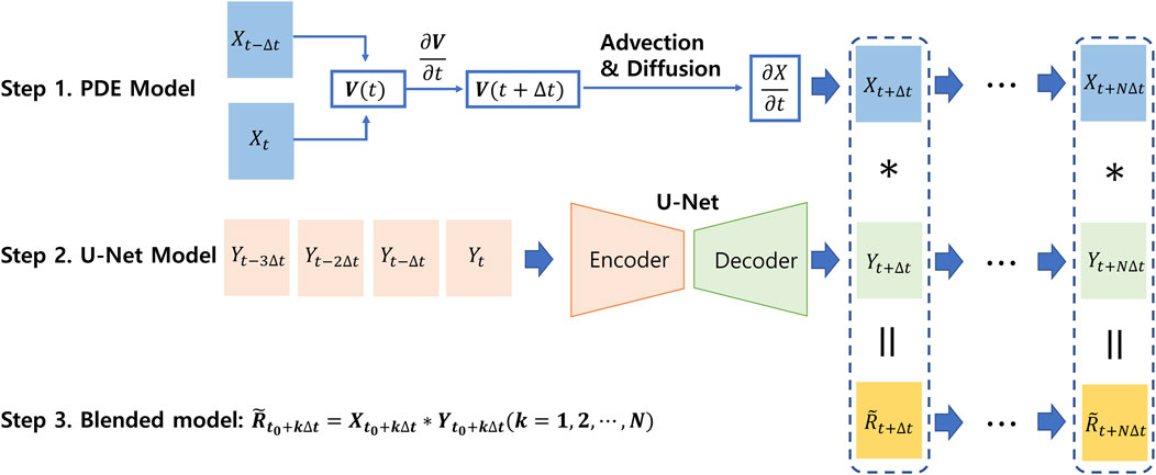
FIGURE 2. A schematic figure of the blended model by combining the PDE and U-Net models. The top and middle panels show the PDE and U-Net models, respectively. Notably, all models produce their prediction fields using a recursive approach, utilizing the previous prediction fields.

2.2.1 Forecasts based on partial differential equations

We adopted the forecast models based on PDEs (PDE model, hereafter) proposed by Ryu et al. (2020). Under the assumption that the motion field of precipitation follows a fluid equation, the model provides nowcasting by solving the advection-diffusion equation and Burgers’ equation in a time-dependent manner. The steps for obtaining nowcasts are as follows: 1) calculating the initial motion field, and 2) solving time-dependent PDEs to obtain nowcasts.

The initial motion field $\mathit{V}\left(\mathit{x}\right)=\left(u,v\right)$ in space $\mathit{x}=\left(x,y\right)$ at time $t_0$ is primarily calculated by the optical flow algorithm. In the optical flow method, the motion field is extracted from two adjacent images in the time domain. Under the assumption that the pixel intensities of an object remain constant, the rainfall intensity $R\left(x+∆x,y+∆y,t+∆t\right)$ can be expressed using a Taylor series:

$R\left(x+∆x,y+∆y,t+∆t\right)-R\left(x,y,t\right)\approx \left(\frac{\partial R}{\partial x}\right)∆x+\left(\frac{\partial R}{\partial y}\right)∆y+\left(\frac{\partial R}{\partial t}\right)∆t,(1)$

when ignoring high-order terms. Dividing the above equation by $∆t$, we obtain

$\frac{R\left(x+∆x,y+∆y,t+∆t\right)-R\left(x,y,t\right)}{∆t}\approx \left(\frac{\partial R}{\partial x}\right)u+\left(\frac{\partial R}{\partial y}\right)v+\left(\frac{\partial R}{\partial t}\right)\approx 0,(2)$

where $u$ and $v$ represent the basic elements of the vector field. As two unknown variables ($u$, $v$) cannot be solved using only one equation, relevant regularization force is required to solve the equation. The total variation-L1 algorithm (TV-L1; Wedel et al., 2009) is used to determine the optical flow by minimizing a regularization force, $J$, defined as follows:

$J\equiv \int \left\{\lambda \left|R_0\left(\mathit{x}\right)-R_1\left(\mathit{x}+\mathit{V}\left(\mathit{x}\right)\right)\right|+\left|\nabla V\right|\right\}dx,(3)$

where $R_0$ and $R_1$ are the rainfall intensities of two different timesteps. The first term is the optical flow constraint, which assumes brightness constancy during motion, and the second term represents the smoothness of displacement fields. TV-L1 is available from the Python public library OpenCV (https://opencv.org).

The motion field obtained by Eqs 1−3 is then updated through the Burgers’ equation, which is expressed as follows,

$\frac{\partial u}{\partial t}=-u\frac{\partial u}{\partial x}-v\frac{\partial u}{\partial y}+\mu \left(\frac{{\partial }^{2}u}{\partial x^2}+\frac{{\partial }^{2}u}{\partial y^2}\right),(4)$

$\frac{\partial v}{\partial t}=-u\frac{\partial v}{\partial x}-v\frac{\partial u}{\partial y}+\mu \left(\frac{{\partial }^{2}v}{\partial x^2}+\frac{{\partial }^{2}v}{\partial y^2}\right),(5)$

where $\mu$ is the kinematic viscosity. The fluid system with a larger viscosity has a smoother motion field. Using the updated motion field, nowcasting is obtained by solving the advection-diffusion equation,

$\frac{\partial R}{\partial t}=-u\frac{\partial R}{\partial x}-v\frac{\partial R}{\partial y}+\nu \left(\frac{{\partial }^{2}R}{\partial x^2}+\frac{{\partial }^{2}R}{\partial y^2}\right),(6)$

where the first term is responsible for advection and the second term is used to describe the diffusion effect with a diffusion coefficient $\nu$. Notably, $\mu$ and $\nu$ are variables varying on the spatial and temporal domains, and were assumed as constants. The values $\mu =0.2$ and $\nu =0.05$ were used, which were empirically determined by Ryu et al. (2020). Additionally, to numerically calculate the derivative, we used the centered difference formula (Wendroff, 1968), which is expressed as follows:

$\frac{\partial R}{\partial x}\approx \frac{R\left(x+∆x\right)-R\left(x-∆x\right)}{2∆x},(7)$

$\frac{{\partial }^{2}R}{\partial x^2}\approx \frac{R\left(x+∆x\right)-2R\left(x\right)+R\left(x-∆x\right)}{{\left(∆x\right)}^2}.(8)$

The Eq. 7 and Eq. 8 were used for solving the partial differential Eqs 4−6.

2.2.2 Forecasts based on the U-Net convolutional neural network

A deep-learning model called RainNet v1.0 was recently proposed by Ayzel et al. (2020) for precipitation nowcasting, wherein the U-Net architecture is adopted, as introduced by Ronneberger et al. (2015). RainNet v1.0 contains four downsampling and four upsampling steps, as shown in Figure 3. During the downsampling steps, the resolution of the input data is reduced by merging every four adjacent pixels, whereras the number of latent features per pixel, representing the pixel’s vector dimension, is doubled. Conversely, in the upsampling steps, the resolution of the input data is doubled, whereas the number of latent features per pixel is halved. To ensure coherence between the downsampling and upsampling steps, skip connections are employed, enabling the intermediate output of each downsampling step (reflecting the vector representation of each pixel) that contributes to the determination of the output of the corresponding upsampling step. The convolutional layers with up to 1,024 filters, kernel sizes of $1\times 1$ and $3\times 3$, and rectified linear unit (ReLU) activation functions were used. Additionally, the dropout layers with the dropout rate = 0.5 were implemented to prevent overfitting. Note that the model parameters were tuned by testing within the following parameter ranges: 1) the number of downsampling and upsampling steps: 3–5; 2) the size of the kernel: $3\times 3$, $5\times 5$, and $7\times 7$; 3) Dropout rates: 0–0.5. For a more comprehensive understanding of the architecture, refer to Ayzel et al. (2020).

FIGURE 3

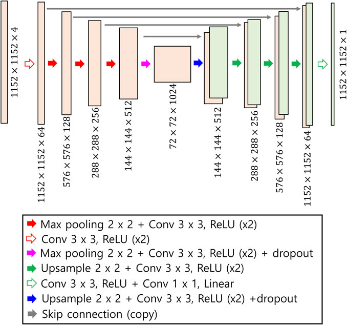
FIGURE 3. The structure of U-Net adopted in this study. The model comprises four downsamplings and four upsamplings. The pixel number of the input image is $\mathbf{1152}\times \mathbf{1152}$ with four channels (i.e., four different timesteps, $\mathit{t}-\mathbf{30}$, $\mathit{t}-\mathbf{20}$, $\mathit{t}-\mathbf{10}$, and $\mathit{t}$), and that of the output image is $\mathbf{1152}\times \mathbf{1152}$ with one channel (i.e., one timestep, $\mathit{t}+\mathbf{10}$).

By employing RainNet v1.0, we obtained the nowcasting outputs, as follows:

${\stackrel{\sim }{R}}_{t+∆t}=p\left(R_{t+∆t}|R_t,R_{t-∆t},R_{t-2∆t},R_{t-3∆t}\right),(9)$

where $R$ and $\stackrel{\sim }{R}$ denote the radar ground truth and prediction, respectively. As a loss function, we adopted the logcosh loss function, $L_{logcosh}$, as follows:

$L_{logcosh}=\frac{{\displaystyle \sum _{i=1}^N}\ln \left(\cosh \left(R_{gt,i}-R_{pred,i}\right)\right)}{N},(10)$

where $R_{gt,i},R_{pred,i}$, and $N$ denote the precipitation fields of ground truth, prediction, and the number of pixels, respectively. To predict the precipitation at $t+∆t$ through Eqs 9, 10, four latest images with $∆t$ interval were used as the input. Notably the spatial resolutions of the input and output are identical, as we used a 1-km interval and $∆t$ of 10 min. We optimized the hyperparameters using 30 epochs with ranges of batch sizes and learning rates, 8–32 and ${10}^{-6}-{10}^{-4}$, respectively. As a set of hyperparameters, we employed the Adam optimizer, with a batch size of 8 and learning rate of ${10}^{-4}$.

2.2.3 Blending the PDE and U-Net models

By combining the forecast from the PDE model ($X_{t_0+k∆t}$) and that from the U-Net model ($Y_{t_0+k∆t}$), the final nowcasting at time $t_0+k∆t\left(k=\mathrm{1,2},\cdots \right)$, ${\stackrel{\sim }{R}}_{t_0+k∆t}=X_{t_0+k∆t}*Y_{t_0+k∆t}$, can be generated. In this study, the blended model is simply defined as ${\stackrel{\sim }{R}}_{t_0+k∆t}=X_{t_0+k∆t}*Y_{t_0+k∆t}=\sqrt{X_{t_0+k∆t}{Y}_{t_0+k∆t}}$. The implication of the characteristics of the blended model is provided below. The time evolution of rainfall intensity, $\partial {\stackrel{\sim }{R}}_{t_0+k∆t}/\partial t$, is expressed as follows:

$\frac{\partial {\stackrel{\sim }{R}}_{t_0+k∆t}}{\partial t}=\frac{1}{2}{\left(\frac{Y_{t_0+k∆t}}{X_{t_0+k∆t}}\right)}^{\frac{1}{2}}\frac{\partial X_{t_0+k∆t}}{\partial t}+\frac{1}{2}{\left(\frac{X_{t_0+k∆t}}{Y_{t_0+k∆t}}\right)}^{\frac{1}{2}}\frac{\partial Y_{t_0+k∆t}}{\partial t}.(11)$

Here, we first assumed that the typical evolution of precipitation is expressed as the advection of the precipitation field and variation of intensity changes owing to the dynamic processes. Under such an assumption, we examined three cases: 1) advection dominant regime: $X_{t_0+k∆t}\gg Y_{t_0+k∆t}$; 2) dynamical processes dominant regime: $X_{t_0+k∆t}\ll Y_{t_0+k∆t}$; and 3) intermediate regime: $X_{t_0+k∆t}\approx Y_{t_0+k∆t}$.

In case that the precipitation field obtained by the PDE model, $X_{t_0+k∆t}$, dominates over $Y_{t_0+k∆t}$, $\partial {\stackrel{\sim }{R}}_{t_0+k∆t}/\partial t$ expressed by the Eq. 11 can be approximately expressed as follows,

$\frac{\partial {\stackrel{\sim }{R}}_{t_0+k∆t}}{\partial t}\approx \frac{1}{2}{\left(\frac{X_{t_0+k∆t}}{Y_{t_0+k∆t}}\right)}^{\frac{1}{2}}\frac{\partial Y_{t_0+k∆t}}{\partial t}.(12)$

Equation 12 indicates the temporal features of U-Net forecasts, and $\partial Y_{t_0+k∆t}/\partial t$ is simultaneously involved when the evolution of precipitation is mainly governed by the evolution of $X_{t_0+k∆t}$. In particular, the growth and decay of precipitation fields can be considered, that are hardly predicted through the PDE model.

When the rainfall intensity obtained by the U-Net model, $Y_{t_0+k∆t}$, is more crucial, $\partial {\stackrel{\sim }{R}}_{t_0+k∆t}/\partial t$ can be simplified as

$\frac{\partial {\stackrel{\sim }{R}}_{t_0+k∆t}}{\partial t}\approx \frac{1}{2}{\left(\frac{Y_{t_0+k∆t}}{X_{t_0+k∆t}}\right)}^{\frac{1}{2}}\frac{\partial X_{t_0+k∆t}}{\partial t}.(13)$

We interpret the Eq. 13 that time variation of $X_{t_0+k∆t}$ can be considered when the U-Net model, $Y_{t_0+k∆t}$ is a dominant forecaster. The main advantage is that the advection features of $X_{t_0+k∆t}$ and precipitation evolution occurring at the small scale could be predicted, which are poorly predicted through the U-Net model.

When the contribution of the two models is comparable, the precipitation field is evolved through both $X_{t_0+k∆t}$ and $Y_{t_0+k∆t}$,

$\frac{\partial {\stackrel{\sim }{R}}_{t_0+k∆t}}{\partial t}\approx \frac{1}{2}\frac{\partial X_{t_0+k∆t}}{\partial t}+\frac{1}{2}\frac{\partial Y_{t_0+k∆t}}{\partial t}.(14)$

The form of $\partial {\stackrel{\sim }{R}}_{t_0+k∆t}/\partial t$ shown in Eq. 14 demonstrates that the precipitation field is evolved by the average evolution of two models.

Notably, during real precipitation evolution, three regimes are simultaneously included. Thus, the blended model could substantially enhance the performance of precipitation nowcasting.

2.2.4 Reference model: Eulerian persistence

As a reference model, we employed Eulerian persistence. Eulerian persistence model (Persistence, hereafter) ensures that the most recent observation is frozen:

$R_{pred,t_0+k∆t}\approx R_{gt,t_0},(15)$

$\frac{\partial R_{{pred,t}_0+k∆t}}{\partial t}\approx 0,(16)$

where $R_{gt,t_0}$ and $R_{pred,t_0+k∆t}$ are the observed and predicted precipitation fields at times $t_0$ and $t_0+k∆t$, respectively. Although this model (Eqs 15, 16) is simple and does not consider the advection or generation and dissipation of the precipitation field, it is powerful for very short lead times. Thus, it has been employed as a baseline model in the recent deep learning-based studies for nowcasting (e.g., Lebedev et al., 2019; Ayzel et al., 2020; Sønderby et al., 2020; Ko et al., 2022).

The purpose of using Persistence can be summarized as follows. The comparison between the PDE model and Persistence enables the evaluation of the accuracy of precipitation nowcasting, considering advection in the precipitation field. By comparing Persistence with the U-Net and the blended models, we can observe the impact of the prediction of the change in precipitation intensity on the accuracy of precipitation nowcasting. Additionally, the comparison between this study and recent studies of deep learning-based precipitation nowcasting can be conducted using Persistence.

3 Results and discussion

This section describes the performance comparison between PDE, U-Net, and blended models. In particular, we report the prediction performance for heavy rainfall events with an accumulated rainfall of $\ge 30mm{h}^{-1}$ within 1 hour, as such events could lead to destructive floods. The evaluation focused on heavy rainfall events during 2022. Both qualitative and quantitative methods were employed to assess the model performance in predicting the motion of precipitation fields and changes in their intensities. Subsequently, we discuss the operational potential of the blended model based on the monthly averaged performance of the blended model.

Figures 4, 5 show the prediction results or precipitation in the central and southern regions of the Korean Peninsula. As demonstrated in previous studies using U-Net (e.g., Ayzel et al., 2020), the U-Net model tends to exhibit significant blurry effects and slightly underestimate the rainfall intensities. Such drawbacks of U-Net predictions are particularly important in certain cases, such as in the example shown in Figure 4, where the stationary rainfall front persists strongly. Conversely, the PDE model overestimates both the spatial extent and rainfall intensities as it fails to accurately simulate the processes such as precipitation dissipation. In particular, PDE-based predictions could provide inaccurate forecasts when encountering precipitation cases with evolving rainfall that dissipates, as shown in the example of Figure 5 (i.e., false alarm rate could increase). In comparison, the blended model performs better than the U-Net and PDE models in tracking the motion of precipitation patterns and accurately predicting dynamical processes, including the dissipation of precipitation and expansion of precipitation areas, in both the central and southern regions.

FIGURE 4

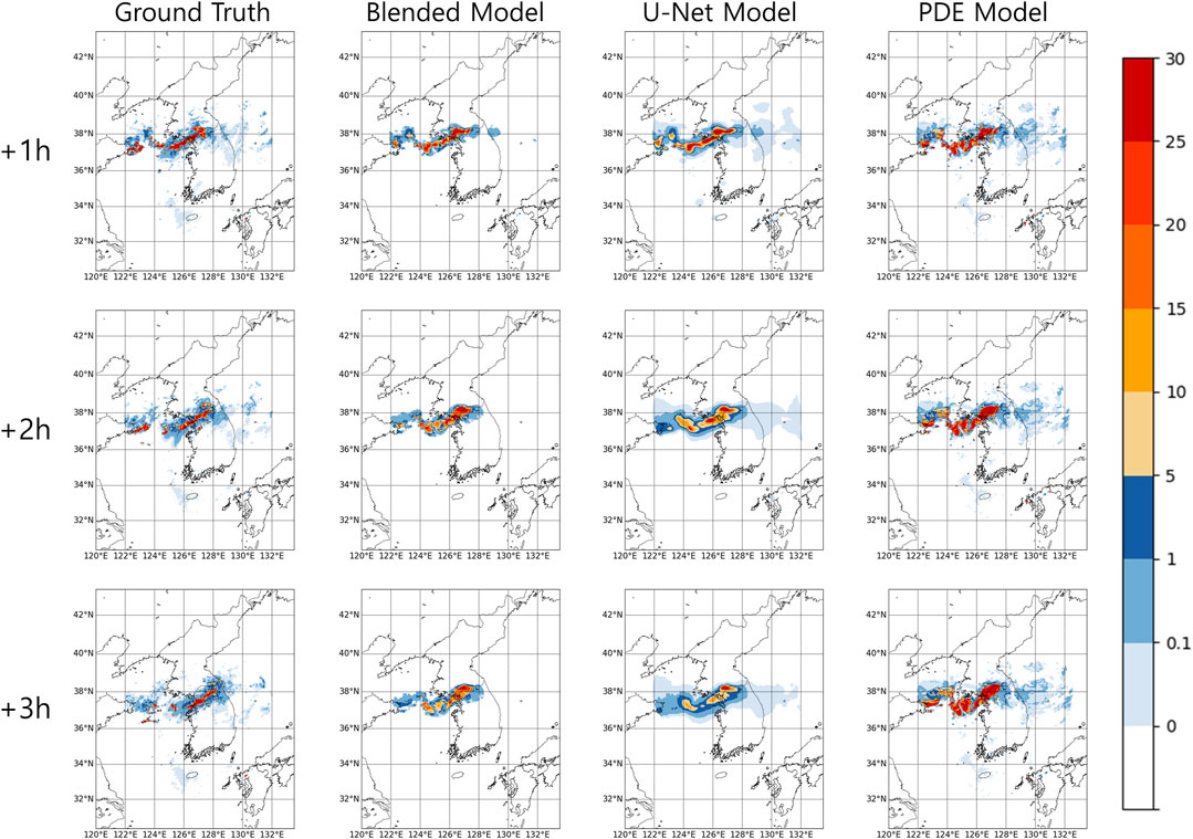
FIGURE 4. Nowcasting outputs of the Central case at 0100 UTC, 8 August 2022 at 0–3-h lead times.

FIGURE 5

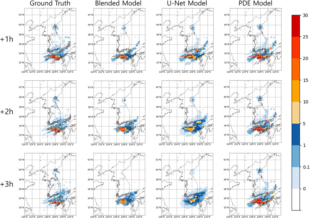
FIGURE 5. Nowcasting outputs of the Southern case at 0200 UTC, 17 August 2022 at 0–3-h lead times.

We also assessed the robustness of the blended model’s performance by predicting heavy rainfall events with characteristics similar to those in Figures 4, 5. The two right panels in Figure 6 demonstrate that the blended model effectively predicts an elongated structure, including convective and stratiform rains, in the Central area. The two left panels in Figure 6 show the performance in predicting the development of the precipitation field in the Southern coastal area. Notably, the blended model accurately forecasts the injection of precipitation from the south-western area, as illustrated in the case at 1200 UTC on 25 April 2022.

FIGURE 6

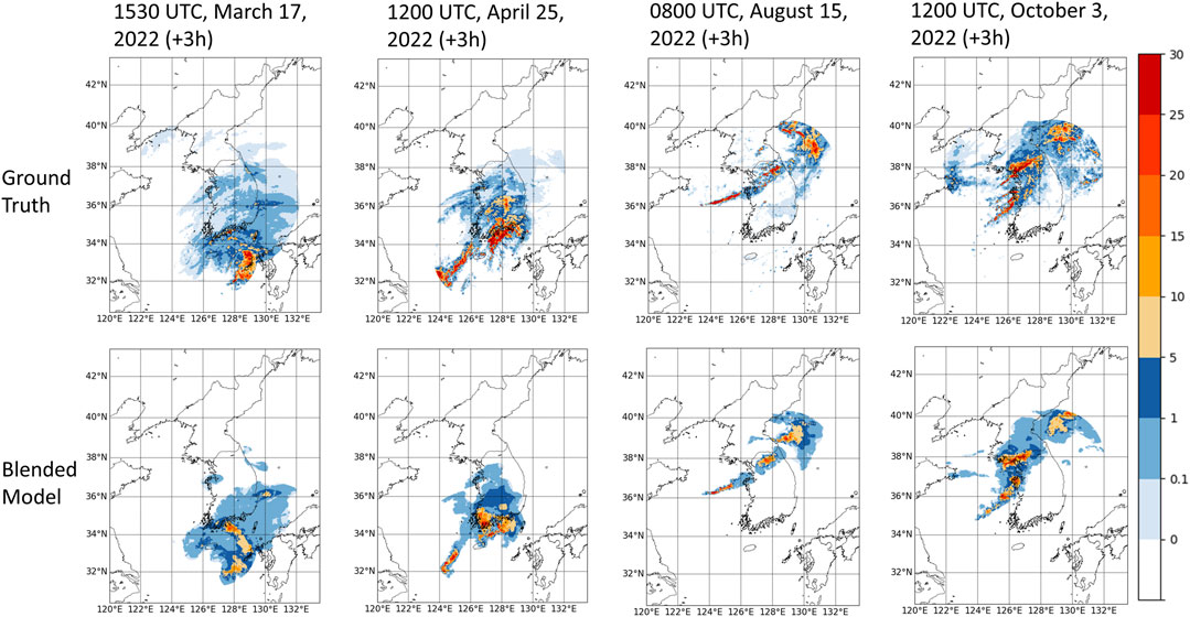
FIGURE 6. Nowcasting outputs of Central (0800 UTC, 15 August 2022; 1200 UTC, 3 October 2022) and Southern (1530 UTC, 17 March 2022; 1200 UTC, 25 April 2022) cases at 3-h lead time.

The blurry effects of the precipitation prediction field were quantitatively measured using power spectral density (PSD) calculations during the 0–3-h lead times. The radially averaged PSD of rainfall intensity is computed as follows:

$\frac{1}{2}{\displaystyle \sum _{i=1}^N}{R}_i^2=\int P\left(k\right)2\pi kdk,(17)$

where $k=\sqrt{k_x^2+k_y^2}$ indicates the radial wavenumber, $N$ is the number of pixels and $R_i$ represents rainfall intensity at individual pixels.

Figure 7 illustrates the results of the PSD calculations using Eq. 17 during the 0–3-h lead times. The PDE model can provide predictions without the loss of spatial information as it considers precipitation advection as a key factor in precipitation pattern evolution. The slight underestimation of the PSD at scales of 10–100 km in the PDE model is attributed to its inability to accurately predict the complex evolution processes observed in real precipitation patterns. For example, the assumptions of constant kinematic viscosity or diffusion coefficient may not adequately represent the intricate details of the actual environment. Additionally, although turbulent motions play a crucial role in precipitation pattern evolution, the motion tracked based on radar data in the two-dimensional space cannot account for the vertical component, which is a limitation. The U-Net model exhibits the blurriest prediction results among the models, whereas the blended model demonstrates less blurriness compared with the U-Net model. Moreover, the power spectrum evolution of the U-Net model shows a decrease in power density at small scales over time, whereas the power spectrum of the blended model maintains consistent power density at small scales, regardless of time. This indicates that the blended model can provide consistent forecasts from the perspective of spatial resolution during 0–3-h lead times.

FIGURE 7

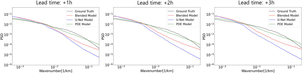
FIGURE 7. Power spectral density (PSD) averaged over 12 heavy rainfall events for 0–3-h lead times. Black, red, blue and green solid lines indicate ground truth, blended, U-Net, and PDE models, respectively.

To investigate the correlation between the predicted ($P$) and observed ($O$) values, the correlation coefficient, $CC$, was estimated using the equation described in Germann and Zawadzki (2002):

$CC\left(O,P\right)=\frac{{\displaystyle \sum _{i=1}^N}{O}_i{P}_i}{\sqrt{{\displaystyle \sum _{i=1}^N}{O}_i^2}\sqrt{{\displaystyle \sum _{i=1}^N}{P}_i^2}}.(18)$

Here, $N$ is the number of pixels; and for calculating $CC$, rainfall intensities and two motion components were considered (i.e., $CC\left(R_{gt},R_{pred}\right),$ $CC\left(u_{gt},u_{pred}\right),$ and $CC\left(v_{gt},v_{pred}\right)$ were calculated). The closer this coefficient is to 1, the higher is the correlation between the predicted and ground truth values, when this value is close to 0, there is almost no correlation.

The evolution of the correlation coefficients of rainfall intensities, $CC\left(R_{gt},R_{pred}\right)$, obtained by Eq. 18, at 0–3-h lead times is shown in Figure 8A. Up to a 1.5-h lead time, U-Net exhibits the highest correlation; however subsequently, the correlation coefficient sharply decreases. This decline indicates that the U-Net model produces overly blurry predictions, resulting in poor correlation with the distribution of ground truth values. Notably, $CC\left(R_{gt},R_{pred}\right)$ of the U-Net model measured at a 3-h lead time is almost comparable with that of Persistence. Conversely, the blended model shows decent performance at 0–3-h lead times, demonstrating the best performance after a 1.5-h lead time. This is attributed to the preservation of spatial resolution and influence of the PDE model, which accounts for the movement of precipitation patterns. Additionally, the blended model captures complex variations in precipitation intensity owing to the U-Net model, leading to a better correlation than the PDE model.

FIGURE 8

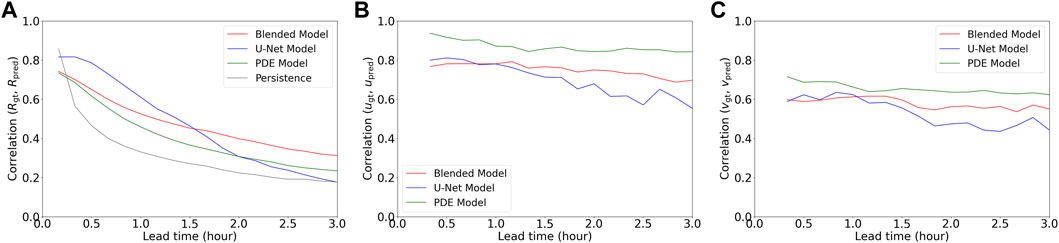
FIGURE 8. Correlation coefficients ($CC$ s) of precipitation fields (A) and two velocity components $\left[u\right.$: (B), $v:$ (C)] averaged over 12 heavy rainfall events for 0–3-h lead times. Red, blue, green and gray solid lines indicate blended, U-Net, PDE models, and Persistence, respectively.

The correlation coefficients of two motion components, $CC\left(u_{gt},u_{pred}\right),$ and $CC\left(v_{gt},v_{pred}\right)$, are displayed in Figures 8B, C. We suggest that compared with those of the U-Net model, the motion fields obtained by the blended model exhibit a better correlation with those obtained by the ground truth. As evident from the PSD analysis shown in Figure 7, this is because the blended model produces less blurry predictions compared with the U-Net model.

To evaluate the accuracy of precipitation prediction, performance was evaluated by measuring critical success index (CSI), probability of detection (POD), and false alarm ratio (FAR). These metrics are defined based on the values of hits ($H$), misses ($M$), and false alarms ($F$) as follows:

$\text{CS}\mathrm{I}=\frac{H}{H+M+F},(19)$

$\text{PO}\mathrm{D}=\frac{H}{H+M},(20)$

$\text{FA}\mathrm{R}=\frac{F}{H+F}.(21)$

The CSI is used to evaluate the accuracy of precipitation prediction (Eq. 19). POD represents the ratio of correctly predicted events among the actual occurrences of precipitation (Eq. 20). A low POD value indicates a higher number of missed events. Higher values (closer to 1) for both CSI and POD indicate more accurate predictions. FAR is used to measure the ratio of incorrectly predicted events out of the total predicted events (Eq. 21). A higher FAR value indicates a larger number of false predictions, often associated with overestimating precipitation areas. A lower FAR value, closer to 0, indicates better predictions.

We evaluated the performance of precipitation events with intensities of $1\text{\hspace{0.17em}mm\hspace{0.17em}}{\mathrm{h}}^{-1}$ or more, $5\text{\hspace{0.17em}mm\hspace{0.17em}}{\mathrm{h}}^{-1}$ or more, and $10\text{\hspace{0.17em}mm\hspace{0.17em}}{\mathrm{h}}^{-1}$ or more. Figure 9 shows the performance evaluation at 0–3-h lead times. In terms of the CSI, the PDE model generally underperforms compared with the other models. This is because it lacks the ability to predict the dynamic processes involved in precipitation evolution. Consistently, the POD values of the PDE model are lower compared with those of the other models (i.e., the number of missed events is higher than those of other models), and larger FAR values indicate a tendency to overestimate rainfall intensities and their areas. The blended model outperforms the other models up to a 3-h lead time, and this improvement is particularly significant when predicting moderate rainfall events ($\ge 1\text{mm\hspace{0.17em}}{\mathrm{h}}^{-1}$). The performance difference between the U-Net and blended models arises from the inability of the U-Net model to predict precipitation advection accurately owing to its blurry effects. These results are consistent with the results of qualitative analysis of Figures 4, 5.

FIGURE 9

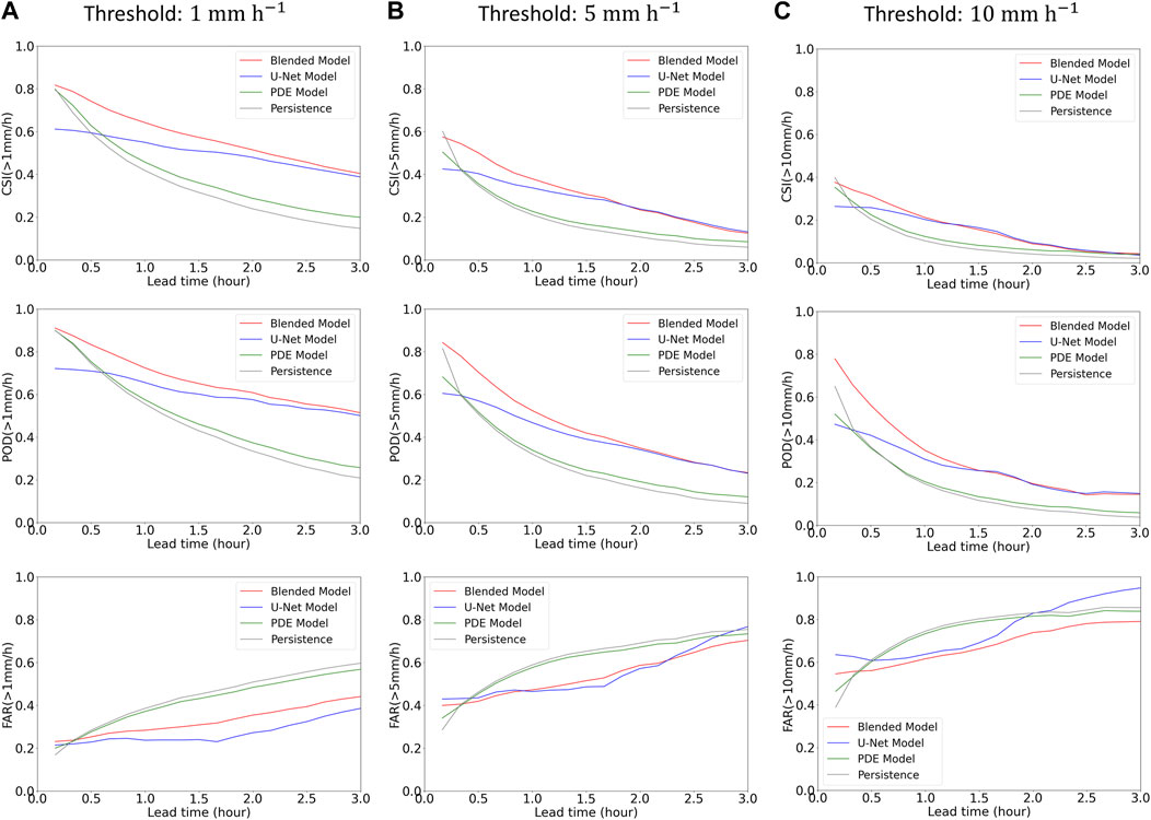
FIGURE 9. Evaluation results (CSI, POD, and FAR) averaged over 12 heavy rainfall events for 0–3-h lead times. The (A–C) show the scores with thresholds of $1$, $5$, and $10\text{\hspace{0.17em}mm\hspace{0.17em}}{\mathrm{h}}^{-1}$, respectively. Red, blue, green and gray solid lines indicate blended, U-Net, PDE models, and Persistence, respectively.

The performance of the blended model was also assessed separately for each precipitation type (i.e., Central and Southern cases) to examine the characteristics of nowcasting outputs produced by the blended model (see Figure 10). Overall, the prediction accuracy for the Central case is higher than that for the Southern case. According to FAR scores, the models generally overestimate when predicting heavy rainfall in the Southern area. Additionally, lower POD values for the Southern case at 1–3-h lead times indicate a substantial number of missing events. We interpret that such performance difference is mainly related to the failure to detect precipitation growth in the southern coastal area. While the blended model accurately predicts the eastward movement of precipitation fields in both the central and southern regions of the Korean Peninsula, dynamic processes such as the growth and decay of precipitation are more prominent in the southern coastal regions. To predict such convective rainfall accurately, additional information such as satellite images would be required, which is beyond the scope of this paper.

FIGURE 10

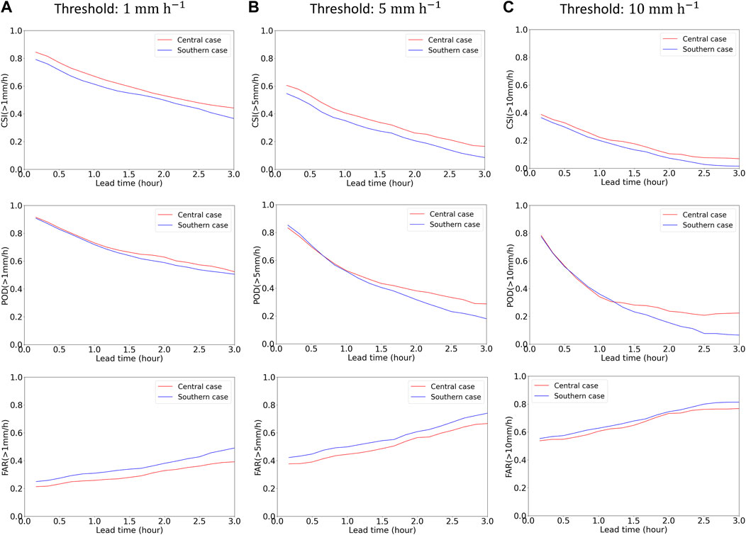
FIGURE 10. Evaluation results (CSI, POD, and FAR) of the blended model for 0–3-h lead times (red: Central case; blue: Southern case). Each precipitation type includes six heavy rainfall events. The (A–C) show the scores with thresholds of $1$, $5$, and $10\text{\hspace{0.17em}mm\hspace{0.17em}}{\mathrm{h}}^{-1}$, respectively.

Comparison between recent studies regarding precipitation nowcasting is presented in Table 1. Notably, direct comparisons cannot be conducted owing to the different detailed settings adopted in each study. Despite such limitations, indirect comparison could be conducted using baselines, such as Persistence and U-Net. In predictions of both moderate ($\ge 1\text{mm\hspace{0.17em}}{\mathrm{h}}^{-1}$) and heavy rainfall ($\ge 10\text{mm\hspace{0.17em}}{\mathrm{h}}^{-1}$), the blended model demonstrates better performance than the other models proposed in previous studies at 0–3-h lead times. Although most previous studies have improved the prediction accuracy through the design and enhancement of deep learning models, we highlight the potential for achieving predictions at higher accuracies by incorporating efficient data processing methods from existing models.

TABLE 1

TABLE 1. Comparison between recent studies of precipitation nowcasting. The CSI scores were used for calculating the improvement over the baseline.

To test the operational feasibility of the blended model, we examined the performance of blended model in predicting precipitation in various seasons, each characterized by distinct weather patterns. We evaluated the monthly-averaged forecast skills based on the CSI scores for different seasons. Figure 11 shows the monthly-averaged performances of the blended and U-Net models during January (i.e., winter season), March (i.e., spring season), and September (i.e., late summer season) 2022, respectively. Notably, the prediction performance during September is the best, whereas it is the worst during January. This is mainly because during summer, more precipitation cases with sustained strong rainfall intensity substantially evolve by advection compared with those in winter or spring. The performances of both the blended and U-Net models follow such seasonal variability. Additionally, the blended model outperforms U-Net in predicting both moderate ($\ge 1\text{mm\hspace{0.17em}}{\mathrm{h}}^{-1}$) and heavy ($\ge 10\text{mm\hspace{0.17em}}{\mathrm{h}}^{-1}$) precipitation events. Hence, we interpret that the performance enhancement of the blended approach is robust for different seasons.

FIGURE 11

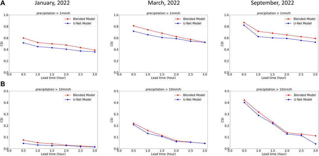
FIGURE 11. CSI results averaged over January, March, and September for 0.5–3-h lead times (red: Blended model; blue: U-Net model). The (A, B) show the scores with thresholds of $1$ and $10\text{\hspace{0.17em}mm\hspace{0.17em}}{\mathrm{h}}^{-1}$, respectively.

4 Summary

In this study, we proposed an approach to improve the performance of existing U-Net models by combining a PDE model that considers fluid dynamics with the U-Net architecture for precipitation prediction. The main objective was to address the blurriness in the predictions from traditional U-Net models. We conducted qualitative and quantitative performance analyses using precipitation cases in the Korean Peninsula. Based on the qualitative and quantitative evaluations, we found that improving the blurriness and enhancing the movement of precipitation patterns through fluid dynamics contribute to the improvement of the prediction accuracy at 0–3-h lead times. In particular, the performance enhancement measured by CSI, POD, and FAR remains robust across different thresholds of rainfall intensity and seasons. Moreover, the blended model demonstrates higher performance compared with PDE-based models that are currently used in operational short-term precipitation forecasting, including KMA’s nowcasting model based on MAPLE. Therefore, the blended model holds potential for future application in operational short-term forecasting. Additionally, the blended model can be easily applied as an extension of existing operational PDE models, providing further advantages.

While this study focused on the strong rainfall events last more than a few hours in the central and southern regions of Korean Peninsula, the prediction accuracy for predicting the isolated precipitation patterns, where rainfall generates or dissipates rapidly in localized areas, is also crucial. Previous deep learning-based studies have also demonstrated relatively poor performance in predicting such isolated precipitation compared with that in predicting precipitation in central and southern cases, which encompass relatively broader regions (Kim and Hong, 2022a; Oh et al., 2023). To further improve the performance of nowcasting models, enhancing the prediction capabilities for isolated precipitation patterns is crucial. As indicated by previous studies (e.g., Miao et al., 2020; Choi et al., 2021), training the data from satellites and surface observations associated with the physical processes of clouds and precipitation would significantly enhance the performance. Such an approach is beyond the scope of this paper, and will be part of future studies.

Data availability statement

The original contributions presented in the study are included in the article/supplementary material, further inquiries can be directed to the corresponding author. The radar data are freely available at the released website of the Korea Meteorological Administration (KMA) (https://data.kma.go.kr/cmmn/main.do).

Author contributions

J-HH: Conceptualization, Investigation, Methodology, Software, Supervision, Validation, Visualization, Writing–original draft. JP: Methodology, Writing–review and editing.

Funding

The author(s) declare financial support was received for the research, authorship, and/or publication of this article. This work was funded by the KMA Research and Development program “Developing AI technology for weather forecasting” under Grant (KMA 2021-00121).

Acknowledgments

The authors thank reviewers for their helpful and constructive comments on the manuscript.

Conflict of interest

The authors declare that the research was conducted in the absence of any commercial or financial relationships that could be construed as a potential conflict of interest.

Publisher’s note

All claims expressed in this article are solely those of the authors and do not necessarily represent those of their affiliated organizations, or those of the publisher, the editors and the reviewers. Any product that may be evaluated in this article, or claim that may be made by its manufacturer, is not guaranteed or endorsed by the publisher.

References

Agrawal, S., Barrington, L., Bromberg, C., Burge, J., Gazen, C., and Hickey, J. (2019). Machine learning for precipitation nowcasting from radar images. Arxiv preprint. Available at: https://arxiv.org/abs/1912.12132.

Google Scholar

Ayzel, G., Heistermann, M., and Winterrath, T. (2019). Optical flow models as an open benchmark for radar-based precipitation nowcasting (rainymotion v0.1). Geosci. Mod. Dev. 12, 1387–1402. doi:10.5194/gmd-12-1387-2019

CrossRef Full Text | Google Scholar

Ayzel, G., Scheffer, T., and Heistermann, M. (2020). RainNet v1.0: a convolutional neural network for radar-based precipitation nowcasting. Geosci. Mod. Dev. 13, 2631–2644. doi:10.5194/gmd-13-2631-2020

CrossRef Full Text | Google Scholar

Bakkay, M. C., Serrurier, M., Burdá, V. K., Dupuy, R., Cabrera-Gutiérrez, N. C., Zamo, M., et al. (2022). Precipitation nowcasting using deep neural network. Arxiv preprint. Available at: https://arxiv.org/abs/2203.13263.

Google Scholar

Benjamin, S. G., DéVényi, D., Weygandt, S. S., Brundage, K. J., Brown, J. M., Grell, G. A., et al. (2004). An hourly assimilation-forecast cycle: the RUC. Mon. Wea. Rev. 132, 495–518. doi:10.1175/1520-0493(2004)132<0495:AHACTR>2.0.CO;2

CrossRef Full Text | Google Scholar

Chen, L., Cao, Y., Ma, L., and Zhang, J. (2020). A deep learning-based methodology for precipitation nowcasting with radar. Earth Space Sci. 7, e2019EA00812. doi:10.1029/2019EA000812

CrossRef Full Text | Google Scholar

Choi, S., and Kim, Y. (2022). Rad-cGAN v1.0: radar-based precipitation nowcasting model with conditional generative adversarial networks for multiple dam domains. Geosci. Model Dev. 15, 5967–5985. doi:10.5194/gmd-15-5967-2022

CrossRef Full Text | Google Scholar

Choi, Y., Cha, K., Back, M., Choi, H., and Jeon, T. (2021). RAIN-F+: the data-driven precipitation prediction model for integrated weather observations. Remote Sens. 13, 3627. doi:10.3390/rs13183627

CrossRef Full Text | Google Scholar

Germann, U., and Zawadzki, I. (2002). Scale-dependence of the predictability of precipitation from continental radar images. Part I: description of the methodology. Mon. Wea. Rev. 130, 2859–2873. doi:10.1175/1520-0493(2002)130<2859:SDOTPO>2.0.CO;2

CrossRef Full Text | Google Scholar

Germann, U., and Zawadzki, I. (2004). Scale-dependence of the predictability of precipitation from continental radar images. Part II: probability forecasts. J. Appl. Meteor. 43, 74–89. doi:10.1175/1520-0450(2004)043<0074:SDOTPO>2.0.CO;2

CrossRef Full Text | Google Scholar

Germann, U., Zawadzki, I., and Turner, B. (2006). Predictability of precipitation from continental radar images. Part IV: limits to prediction. J. Atmos. Sci. 63, 2092–2108. doi:10.1175/JAS3735.1

CrossRef Full Text | Google Scholar

Jo, E., Park, C., Son, S. W., Roh, J. W., Lee, G. W., and Lee, Y. H. (2020). Classification of localized heavy rainfall events in South Korea. Asia-Pacific J. Atmos. Sci. 56, 77–88. doi:10.1007/s13143-019-00128-7

CrossRef Full Text | Google Scholar

Kim, Y., and Hong, S. (2022a). Very short-term prediction of weather radar-based rainfall distribution and intensity over the Korean peninsula using convolutional long short-term memory network. Asia-Pac. J. Atmos. Sci. 58, 489–506. doi:10.1007/s13143-022-00269-2

CrossRef Full Text | Google Scholar

Kim, Y., and Hong, S. (2022b). Very short-term rainfall prediction using ground radar observations and conditional generative adversarial networks. IEEE Trans. Geoscience Remote Sens. 60, 1–8. doi:10.1109/TGRS.2021.3108812

CrossRef Full Text | Google Scholar

Ko, J., Lee, K., Hwang, H., Oh, S. G., Son, S. W., and Shin, K. (2022). Effective training strategies for deep-learning-based precipitation nowcasting and estimation. Comput. Geosci. 161, 105072. doi:10.1016/j.cageo.2022.105072

CrossRef Full Text | Google Scholar

Korea Meteorological Administration (KMA) (2021). Abnormal climate report 2020 (in Korean). Available at: http://www.climate.go.kr/home/bbs/view.php?code=93&bname=abnormal&vcode=6494.

Google Scholar

Kox, T., Gerhold, L., and Ulbrich, U. (2015). Perception and use of uncertainty in severe weather warnings by emergency services in Germany. Atmos. Res. 158-159, 292–301. doi:10.1016/j.atmosres.2014.02.024

CrossRef Full Text | Google Scholar

Kwon, S., Jung, S. H., and Lee, G. (2015). Inter-comparison of radar rainfall rate using Constant Altitude Plan Position Indicator and hybrid surface rainfall maps. J. Hydrology 531, 234–247. doi:10.1016/j.jhydrol.2015.08.063

CrossRef Full Text | Google Scholar

Lebedev, V., Ivashkin, V., Rudenko, I., Ganshin, A., Molchanov, A., Ovcharenko, S., et al. (2019). “Precipitation nowcasting with satellite imagery,” in Proceedings of the 25th ACM SIGKDD International Conference on Knowledge Discovery & Data Mining, 2680–2688. doi:10.1145/3292500.3330762

CrossRef Full Text | Google Scholar

Lee, D.-K., Ha, J.-C., and Kim, J. (2008). Application of the Sawyer-Eliassen equation to the interpretation of the synoptic-scale dynamics of a heavy rainfall case over East Asia. Asia-Pac. J. Atmos. Sci. 44, 49–68.

Google Scholar

Lee, H. C., Lee, Y. H., Ha, J.-C., Chang, D.-E., Bellon, A., Zawadzki, I., et al. (2010). McGill algorithm for precipitation nowcasting by Lagrangian extrapolation (MAPLE) applied to the southSouth Korean radar network. Part II: real-time verification for the summer season. Asia-Pacific J. Atmos. Sci. 46, 383–391. doi:10.1007/s13143-010-1009-9

CrossRef Full Text | Google Scholar

Lyu, G., Jung, S. H., Nam, k.Y., Kwon, S., Lee, C. R., and Lee, G. (2015). Improvement of radar rainfall estimation using radar reflectivity data from the hybrid lowest elevation angles. J. Korean Earth Sci. Soc. 36, 109–124. doi:10.5467/JKESS.2015.36.1.109

CrossRef Full Text | Google Scholar

Lyu, G., Jung, S. H., Oh, Y., Park, H. M., and Lee, G. (2017). Accuracy evaluation of composite hybrid surface rainfall (HSR) using KMA weather radar network. J. Korean Earth Sci. Soc. 38, 496–510. doi:10.5467/JKESS.2017.38.7.496

CrossRef Full Text | Google Scholar

Miao, K., Wang, W., Hu, R., Zhang, L., Zhang, Y., Wang, X., et al. (2020). Multimodal semisupervised deep graph learning for automatic precipitation nowcasting. Math. Probl. Eng. 2020, 1–9. doi:10.1155/2020/4018042

CrossRef Full Text | Google Scholar

Oh, S. G., Park, C., Son, S. W., Ko, J., Shin, K., Kim, S., et al. (2023). Evaluation of deep-learning-based very short-term rainfall forecasts in South Korea. Asia-Pacific J. Atmos. Sci. 59, 239–255. doi:10.1007/s13143-022-00310-4

CrossRef Full Text | Google Scholar

Park, C., Son, S. W., Kim, J., Chang, E. C., Kim, J. H., Jo, E., et al. (2021). Diverse synoptic weather patterns of warm-season heavy rainfall events in South Korea. Mon. Wea. Rev. 149, 3875–3893. doi:10.1175/MWR-D-20-0388.1

CrossRef Full Text | Google Scholar

Pulkkinen, S., Nerini, D., Perez Hortal, A. A., Velasco-Forero, C., Seed, A., Germann, U., et al. (2019). Pysteps: an open-source Python library for probabilistic precipitation nowcasting (v1.0). Geosci. Mod. Dev. 12, 4185–4219. doi:10.5194/gmd-12-4185-2019

CrossRef Full Text | Google Scholar

Ravuri, S., Lenc, K., Willson, M., Kangin, K., Lam, R., Mirowski, P., et al. (2021). Skilful precipitation nowcasting using deep generative models of radar. Nature 597, 672–677. doi:10.1038/s41586-021-03854-z

PubMed Abstract | CrossRef Full Text | Google Scholar

Ronneberger, O., Fischer, P., and Brox, T. (2015). “U-net: convolutional networks for biomedical image segmentation,” in International Conference on Medical Image Computing and Computer-Assisted Intervention, 234–241. doi:10.1007/978-3-319-24574-4_28

CrossRef Full Text | Google Scholar

Ryu, S., Lyu, G., Do, Y., and Lee, G. (2020). Improved rainfall nowcasting using Burgers’ equation. J. Hydrology 581, 124140. doi:10.1016/j.jhydrol.2019.124140

CrossRef Full Text | Google Scholar

Seo, K.-H., Son, J.-H., Lee, J.-Y., and Park, H.-S. (2015). Northern East Asian monsoon precipitation revealed by airmass variability and its prediction. J. Clim. 28, 6221–6233. doi:10.1175/JCLI-D-14-00526.1

CrossRef Full Text | Google Scholar

Shi, X., Chen, Z., Wang, H., Yeung, D.-Y., Wong, W.-K., and Woo, W.-C. (2015). Convolutional lstm network: a machine learning approach for precipitation nowcasting. Adv. Neural Inf. Process. Syst. 28.

Google Scholar

Shi, X., Gao, Z., Lausen, L., Wang, H., and Yeung, D.-Y. (2017). Deep learning for precipitation nowcasting: a benchmark and A new model. Adv. Neural Inf. Process. Syst. 30.

Google Scholar

Shrestha, D., Robertson, D., Wang, Q., Pagano, T., and Hapuarachchi, H. (2013). Evaluation of numerical weather prediction model precipitation forecasts for short-term streamflow forecasting purpose. Hydrology Earth Syst. Sci. 17, 1913–1931. doi:10.5194/hess-17-1913-2013

CrossRef Full Text | Google Scholar

Sivle, A. D., Agersten, S., Schmid, R., and Simon, A. (2022). Use and perception of weather forecast information across Europe. Meteorol. Appl. 29, e2053. doi:10.1002/met.2053

CrossRef Full Text | Google Scholar

Sønderby, C. K., Espeholt, L., Heek, J., Dehghani, M., Oliver, A., Salimans, T., et al. (2020). Metnet: a neural weather model for precipitation forecasting. arXiv preprint. doi:10.48550/arXiv.2003.12140

CrossRef Full Text | Google Scholar

Sun, J., Xue, M., Wilson, J. W., Zawadzki, I., Ballard, S. P., Onvlee-Hooimeyer, J., et al. (2014). Use of NWP for nowcasting convective precipitation: recent progress and challenges. Bull. Am. Meteorological Soc. 95, 409–426. doi:10.1175/BAMS-D-11-00263.1

CrossRef Full Text | Google Scholar

Thorndabl, S., Einfalt, T., Willems, P., Nielsen, J. E., Veldhuis, M.-C., Arnbjerg-Nielsen, K., et al. (2017). Weather radar rainfall data in urban hydrology. Hydrol. Earth Syst. Sci. 21, 1359–1380. doi:10.5194/hess-21-1359-2017

CrossRef Full Text | Google Scholar

Turner, B. J., Zawadzki, I., and Germann, U. (2004). Predictability of precipitation from continental radar images. Part III: operational nowcasting implementation (MAPLE). J. Appl. Meteor. 5, 231–248. doi:10.1175/1520-0450(2004)043<0231:POPFCR>2.0.CO;2

CrossRef Full Text | Google Scholar

Wang, G., Yang, J., Wang, D., and Liu, L. (2016). A quantitative comparison of precipitation forecasts between the storm-scale numerical weather prediction model and auto-nowcast system in Jiangsu, China. Atmos. Res. 181, 1–11. doi:10.1016/j.atmosres.2016.06.004

CrossRef Full Text | Google Scholar

Wedel, A., Pock, T., Zach, C., Bischof, H., and Cremers, D. (2009). An improved algorithm for TV-L1 optical flow. Stat. geometrical approaches Vis. motion analysis, 23–45. doi:10.1007/978-3-642-03061-1_2

CrossRef Full Text | Google Scholar

Wendroff, B. (1968). Difference methods for initial-value problems (Robert D. Richtmyer and K. W. Morton). SIAM Rev. 10, 381–383. doi:10.1137/1010073

CrossRef Full Text | Google Scholar

Yu, W., Yoon, S., Choi, M., and Jung, K. (2017). Performance comparison of rainfall and flood forecasts using short-term numerical weather prediction data from Korea and Japan. J. Korea Water Resour. Assoc. 50, 537–549. doi:10.3741/JKWRA.2017.50.8.537

CrossRef Full Text | Google Scholar