 Michiel Arts
 Carlo Corradini2
 Monica Pondrelli
 Damien Pas
 Anne-Christine Da Silva
- 1Sedimentary Petrology, Geology Department, Liège University, Liège, Belgium
- 2Dipartimento di Matematica e Geoscienze, Università di Trieste, Trieste, Italy
- 3International Research School of Planetary Sciences, Pescara, Italy
- 4Dipartimento di Ingegneria e Geologia, Università d’Annunzio, Pescara, Italy
- 5Institute of Earth Sciences (ISTE), University of Lausanne, Lausanne, Switzerland
The type-Silurian Cellon section in the Carnic Alps in Austria underpins much of the current Silurian conodont zonations, forming the basis for the Silurian timescale. However, the Silurian record of the Cellon section lacks radiometric and astrochronological age constraints, making it difficult to gain insights into the processes pacing Silurian (anoxic) events. To attain age constraints and investigate the pacing Silurian (anoxic) events by astronomical cycles, a cyclostratigraphic study was conducted on high-resolution pXRF (CaO, Al2O3, and Fe2O3) and induration records spanning the Ludlow and Pridoli parts of the Cellon section. Astronomical cycles ranging from precession to the 405-kyr eccentricity cycle were first recognised visually in the field and in proxy records. The visual detection of astronomical cycles served as an input for the WaverideR R package, enabling the tracking of the 405-kyr eccentricity period in each proxy’s continous wavelet transform scalograms. These tracked period curves were combined with external age controls through multiple Monte Carlo simulations, generating an (absolute) age model. This age model is used to assign ages and durations and their respective uncertainties to a hiatus in the Ludfordian, conodont zones, lithological units, geochronological units and events, yielding new ages for Silurian stage boundaries (e.g., Gorstian-Ludfordian boundary at 425.92 ± 0.65 Ma, the Ludfordian-Pridoli boundary at 423.03 ± 0.53 Ma, the Silurian-Devonian boundary at 418.86 ± 1.02 Ma), and new durations for the Ludfordian at 2.89 ± 0.35 Myr and Pridoli at 4.24 ± 0.46 Myr. Furthermore, the imprint of astronomical cycles in the Cellon section itself indicates that the Linde, Klev and Silurian-Devonian boundary events all occur after a 2.4-Myr eccentricity node, indicating pacing by astronomical forcing, similar to other Devonian and Cretaceous anoxic events. The Lau event, however, does not appear to coincide with a 2.4-Myr eccentricity node.
1 Introduction
The Silurian period, although the shortest in the Palaeozoic era, is one of the most dynamic. This is evidenced by some of the largest δ13C excursions of the Phanerozoic, which are associated with climatic changes, elevated species turnover rates, and significant facies shifts associated with strong changes in sedimentation rates (Calner, 2004; Cooper et al., 2014; McLaughlin et al., 2018, 2019; Cramer and Jarvis, 2020; Jarochowska et al., 2021). Assessing the trigger of these δ13C excursions and their associated events is challenging due to the quality of the Silurian time scale. Correlating exact time equivalent events from different settings and providing durations and rates for those specific events remains problematic. The uncertainties on the Silurian time scale are rather large, particularly those of the upper Silurian. For example, the uncertainty is ±1.5 Myr for the base of the Gorstian and Ludfordian and ±1.6 Myr for the base of the Pridoli. At the same time, these Stages are rather short (Gorstian duration estimated at 1.7 Myr, Ludfordian 2.3 Myr and Pridoli 2.3 Myr) (Melchin et al., 2020).
Astrochronologies have been used to refine and reduce the uncertainty of the geological timescale (Hinnov and Hilgen, 2012; Hinnov, 2018; Huang, 2018). Although sparse compared to the rest of the Phanerozoic, Silurian cyclostratigraphic studies have been conducted [see Wu et al. (2023) for a compilation]. Still, most of the Silurian period is not yet covered by (floating) astrochronologies. Furthermore, none of the Silurian cyclostratigraphic studies is anchored to absolute ages, and such cyclostratigraphic studies have not yet been used to refine the absolute ages of the Silurian timescale (Melchin et al., 2020). Besides providing age constraints, cyclostratigraphy can be used to make inferences about past climate dynamics (Hinnov, 2013). Whether astronomical pacing was enough to pace some of the Silurian’s large carbon isotopic spikes and associated (anoxic) events remains unknown. But previous studies have suggested that the Upper Kellwasser (Late Devonian) and the Oceanic Anoxic Event II occurred after a 2.4-Myr eccentricity minimum (Batenburg et al., 2016; De Vleeschouwer et al., 2017; Da Silva et al., 2020). As such, it might be possible that astronomical cycles also paced Silurian (anoxic) events.
In this study, an anchored astrochronology will be constructed for the Ludlow (upper Silurian) to lowermost Lochkovian (Devonian) part of the Cellon section in the Carnic Alps to put new (absolute) age constraints on the upper Silurian and also study the role that the 2.4-Myr eccentricity cycle could have played in pacing Silurian (anoxic) events. This portion of the Cellon section has one of the best-constrained conodont biostratigraphies of the Silurian and only contains one significant hiatus, spanning the upper part of the P. siluricus and the lower part of the Pe. latialata/Oz. snajdri interval conodont zones (Walliser, 1964; Corradini et al., 2015, 2022; Corriga et al., 2016) (Figure 1).
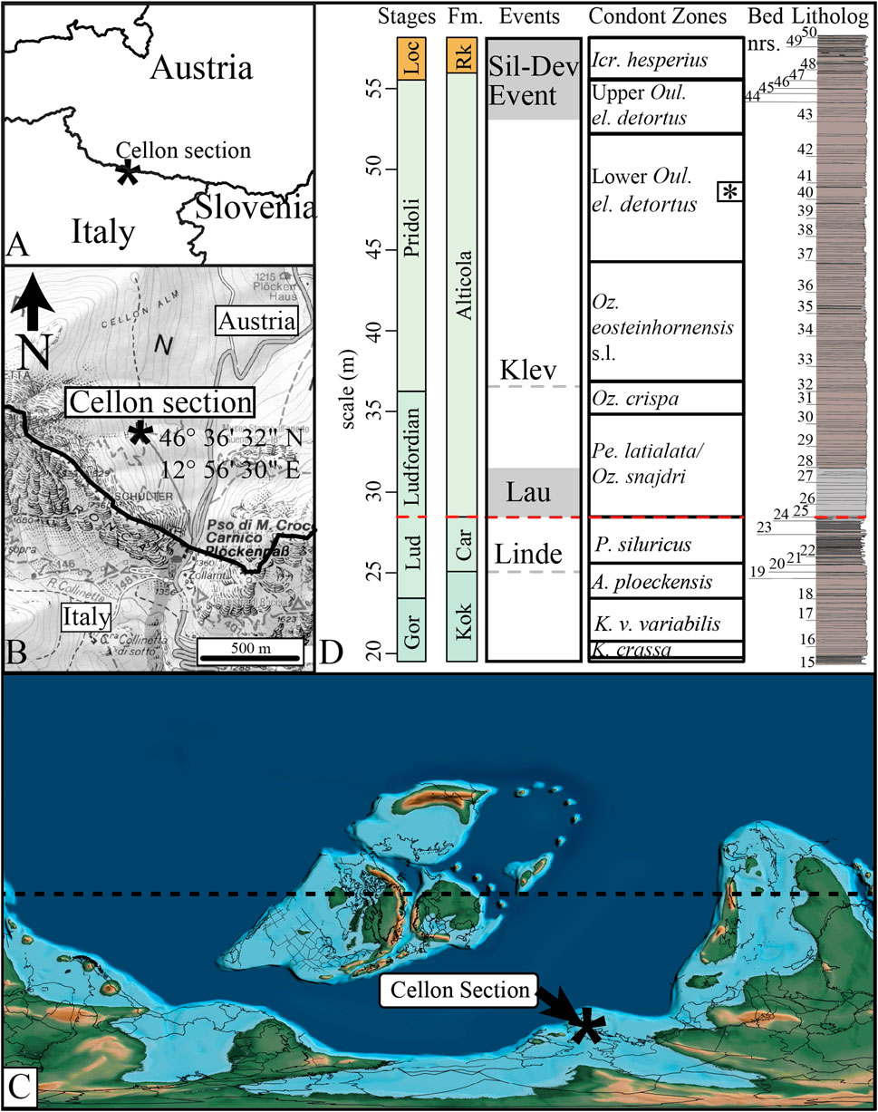
Figure 1. Location, lithological column and palaeogeography of the Cellon section. (A) and (B) location of the Cellon section (46° 36′32″N 12° 56′30″E) modified after Corradini et al. (2017), (C) paleogeographic location of the Cellon section during the Ludlow (modified after Scotese (2021) (D), from left to right stages Loc =Lochkovian, Formations Car = Cardiola and RK = Rauchkofel, Events based on Wenzel (1997), Jeppsson and Aldridge (2000), Brett et al. (2009) and Histon (2012a, 2012b), Conodont zonation (Corradini et al., 2015, 2022), bed numbers of (Walliser, 1964) and lithology [(digitised of (Walliser, 1964)]. The dashed red line in (D) is a hiatus identified through biostratigraphy (see text in the geological setting). * indicates the Oz. eosteinhornensis s.s. horizon.
This cyclostratigraphic study will introduce and subsequently leverage the functions of the WaverideR R package (Arts, 2023) to conduct a cyclostratigraphic study on the (digitised) litholog of Walliser (1964) and on a 1-cm resolution pXRF record. The study will also integrate the (digitised) δ13Ccarb record of Wenzel (1997), as well as the conodont zonation (Walliser, 1964; Corradini et al., 2015, 2020, 2022; Corriga et al., 2016). In the first step of the study, the visual imprint of cycles will first be described for the litholog and pXRF records. Then, an anchored age model with its uncertainties is built through multiple steps of wavelet-based age modelling approach and Monte Carlo simulations (WaverideR) by combining multiple proxy records with an absolute radiochronologic date of Cramer et al. (2015), with the estimated duration of the hiatus. This anchored age model provides a precise time scale with uncertainties for the upper Silurian.
The studied interval in the Cellon section also contains the Linde, Lau Klev and Silurian-Devonian boundary events. The 2.4-Myr astronomical cycle extracted from the newly built age model, will be used to shed on the very long eccentricity cycle’s role in pacing Silurian events.
2 Geological setting
The Cellon section is part of the pre-Variscan sequence of the Carnic Alps (Figures 1A, B). During the Silurian period, the Carnic Alps were part of the Galatian superterrane, which was located around 35°S (Schönlaub, 1992; von Raumer and Stampfli, 2008; Scotese, 2021) (Figure 1C). The Silurian succession of the Carnic Alps was deposited in a basin with roughly a northwest-to-southeast deepening trend (Schönlaub, 1979; Jaeger and Schönlaub, 1980; Wenzel, 1997).
The Cellon section exposes rocks from the Katian to the Lochkovian, belonging to seven Formations: from base to top, Valbertad, Uqua, Plöcken, Kok, Cardiola, Alticola and Rauchkofel Formations (Corradini and Pondrelli, 2021 and reference therein). The Silurian part is represented by the Kok, Cardiola and Alticola Formations (Figure 1D). These Formations belong to the regional “Plöcken facies type” consisting of a conformable limestone sequence interspersed by shales/marls intervals and beds deposited in a stable depositional environment (Schönlaub et al., 1994; Brett et al., 2009). Despite the conformable nature of the succession, some depositional gaps have been observed (Schönlaub, 1979; Jaeger and Schönlaub, 1980; Wenzel, 1997). The following Formations have been studied in this paper and are documented in Figure 1D.
The Kok Formation is of Llandovery to the earliest Ludlow age. It comprises well-bedded brownish ferruginous nautiloid-bearing limestones, alternating with black shales and marly interbeds. The Formation has a thickness of 13.5 m and spans beds 9–19 and the P. celloni SZ to A. ploeckensis conodont zones. The Cellon section’s Gorstian part covers beds 15–19 and has a thickness of 5.58 m. According to Corradini et al. (2015), the Homerian-Gorstian boundary in the Cellon record is located at 19.5 m, at the top of bed 15A. The base of the Gorstian boundary is identified by the first occurrence of K. crassa in bed 15B1. Between beds 15A and 15B1, there is a highly condensed interval of about 25 cm of marly shales. This interval may contain a hiatus, as the two uppermost biozones of the Homerian are not documented in the Cellon section (Jaeger and Schönlaub, 1980; Corradini et al., 2015).
The Cardiola Formation spans the early Ludfordian and comprises dark grey to black limestones with marly and shaly interbeds. The Cardiola Formation spans beds 20–24, has a thickness of 3.39 m, and includes the uppermost part of the A. ploeckensis and the P. siluricus conodont zones (Corradini et al., 2015, 2022). In the Cellon section, the upper part of the P. siluricus zone is absent, indicating a hiatus between the Cardiola and Alticola Formations (Corradini et al., 2015, 2022). The boundary of the Kok and Cardiola Formations (25.08 m) aligns with the Linde Event (Jeppsson and Aldridge, 2000; Histon, 2012a, 2012b). The Linde Event is poorly constrained, so only a midpoint at 25.08 m is assigned to it.
The Alticola Formation spans the middle Ludfordian to the early Lochkovian. It comprises grey to pinkish nautiloid-bearing limestones interbedded by the occasional marl/shale layer and coarse bioclastic interbeds. The Formation spans beds 25-47B, with a thickness of 27.5 m and covers the Pe. latialata/Oz. snajdri to the Icr. hesperius conodont zones. The Silurian-Devonian boundary is located between beds 47A and 47B (55.54 m). The Alticola Formation in the Cellon section contains three events. The Lau event spans beds 25 to 27 (28.47 and 31.48 m). The Klev event is poorly constrained, so only a midpoint at 36.6 m is assigned to the event. The Silurian-Devonian event starts in bed 43 (at 52.9 m) and continues into the overlying Rauchkofel Formation (Wenzel, 1997; Jeppsson and Aldridge, 2000; Histon, 2012a, 2012b).
The Rauchkofel Formation is a lower Lochkovian limestone formation that contains black marl and shale interbeds. The Formation is rich in graptolites, which decrease towards the top. At the Cellon mountain locality, the Rauchkofel Formation has a thickness of ∼170 m (Pondrelli et al., 2020), but only the lower 20 m are accessible in the Cellon section (Corriga et al., 2016). This study is limited to the basal section of the Rauchkofel Formation (beds 47C-50), which has a cumulative thickness of 2.19 m and belongs to the Icr. hesperius zone. The Rauchkofel Formation included in this research is part of the Silurian-Devonian event (Wenzel, 1997; Brett et al., 2009; Histon, 2012b, 2012a).
3 Material and methods
3.1 Dataset acquisition
This study investigates the Ludlow to lowest Lochkovian part of the Cellon section, specifically the interval between beds 15 to 50, which spans from 19.5 to 58.16 m according to the scale of Walliser (1964). During the summer of 2021, samples were taken every centimetre between Bed 15 and 32A, spanning from 19.5 to 40.15 m, while the interval between 40.16 and 58.16 m was studied using the induration record of Walliser (1964).
The collection process involved cutting two perpendicular grooves into the outcrop using an angle grinder. Block samples were removed with a hammer and chisel (Figure 5B). Depth marks were drawn on these block samples and then cut into centimetre-thick blocks using a bench grinder. Shales and marly/soft limestones were chiselled out centimetre by centimetre using a mini stone chisel. All samples with sufficient integrity were ground to achieve a planar, clean surface, allowing for measurements using a portable X-ray fluorescence spectrometer (pXRF). Crumbly or fragmented samples were dried in an oven at 60°C for 1 week and then ground into a fine powder using an agate ball mill. The resulting powder was placed in plastic cups covered with Mylar® thin film. A total of 2020 samples were collected and prepared.
The filled cups and prepared samples were measured using a Bruker Tracer 5g pXRF (Liege University, Belgium) equipped with a 4 W, 200 μA and 50 kV X-ray source, a 1 μm graphene window and an 8 mm collimator, with a resolution < 140 eV at 250,000 cps. All measurements were taken in ambient air using an 8 mm collimator without an additional filter. The energy selected for the measurement was 40 keV, with a current of 20 μA, for 75 s. The calibration uses an in-house calibration made with 17 Certified Reference Material pellets, using the Bruker calibration tool EasyCal [see Da Silva et al. (2023) for further details]. The measured sample stratigraphic heights were adjusted to Walliser’s (1964) reference scale, resulting in an average spacing of 0.907 cm. The CaO, Al2O3 and Fe2O3 proxies were selected for spectral analysis.
In addition to the pXRF geochemical, the litholog of Walliser (1964) and the δ13Ccarb dataset of Wenzel (1997) were digitised using the Log Evolve type log digitising software and Adobe Illustrator. The litholog was rescaled to a range of 1–5, resulting in an induration record. The δ13Ccarb dataset was used to identify δ13Ccarb variations that may have resulted from global (biotic) events (Figure 2). The conodont zonations described by Walliser (1964) and Corradini et al. (2015, 2020, 2022); Corriga et al. (2016) are utilised to identify hiatuses and establish stage boundaries. Figure 2 presents these proxies and the associated data from the Cellon section.
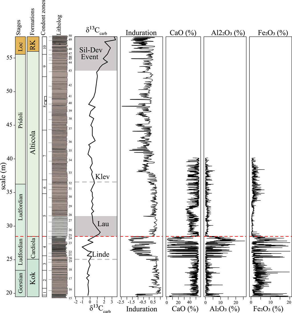
Figure 2. Data used in this study. Stage boundaries (Loc = Lochkovian), Formation (RK = Rauchkofel), conodont zonation, lithology including bed numbers, digitised after Walliser (1964), δ13Ccarb record (Wenzel, 1997) overlain by Silurian events [based on Wenzel, 1997; Jeppsson and Aldridge, 2000; Brett et al., 2009; Histon, 2012a, 2012b)]. Induration record, CaO, Al2O3 and Fe2O3. Numbers 1–10 correspond to the conodont zones K. crassa (1)., K.v. variabilis (2), A. ploeckensis (3), P. siluricus (4), Pe. latialata/Oz. snajdri (5), Oz. crispa (6), Oz. eosteinhornensi s.l. (7), Lower Oul. el. detortus (8), Upper Oul. el. detortus (9) Icr. hesperius (10) and * indicates the Oz. eosteinhornensis s.s. horizon. The red line corresponds to the location of a known hiatus (Corradini et al., 2015, 2022).
3.2 Spectral analysis—Integrated wavelet-based spectral analysis using the WaverideR R package
This section introduces a six-stepped approach using the functions of the WaverideR R package (see Supplementary Material S7 for the R code). The workflow combines the continuous wavelet transform (CWT) with Monte Carlo simulations, resulting in an anchored astrochronology. In the first step (1), the visually observed cyclicity is compared to the cycles observed in the scalograms of the different proxy records’ CWTs. The observed cycles are then linked to their corresponding astronomical cycles, followed by tracking the period of the stable 405-kyr cycle in wavelet scalograms. In step (2), a Monte Carlo simulation combines multiple tracked period (m) curves of the 405-kyr eccentricity into a single tracked period (m) with uncertainty. In step (3), the analytical uncertainty of the wavelet is used to assign an uncertainty to the tracked period (m) curve of the 405-kyr eccentricity cycle curve when only a single tracked 405-kyr cycle curve is available. In step (4), the stable nature of the 405-kyr eccentricity cycle duration is used in a Monte Carlo simulation to calculate the duration of the gap spanning the missing upper part of the P. siluricus and the lower part of the Pe. latialata/Oz. snajdri interval conodont zones in the Cellon section. Step (5) involves combining the cyclostratigraphic time scale (including uncertainty and hiatus duration) with one absolute radiochronologic date (including uncertainty) of Cramer et al. (2015) in a Monte Carlo simulation to generate an anchored astrochronological timescale. This timescale is then used to assign absolute ages and durations, including uncertainties, to Silurian geochronological units, lithological units, and biozones. In step (6), the proxy data in the absolute time domain is analysed using the CWT, followed by the extraction of astronomical cycles from the tuned proxy records to shed light on the 2.4 Myr eccentricity cycle’s role in pacing Silurian events.
3.2.1 Visual analysis and pre-processing
Before conducting any spectral analysis, a visual inspection is carried out to determine if there is any stratigraphic hierarchy or bundling of cycles in the proxy record and outcrop images between lithologies or the stacking of beds of similar thicknesses and whether this bundling can be linked to astronomical forcing. The identified hierarchy of bundling of cycles aims to identify the primary cyclicity in the bedding alternations. The order of cycles, as identified in the Cellon section, will be described from a cyclostratigraphic point of view and will not adhere to the order of cycles as is commonly used in sequence stratigraphic studies. Consequently, the observed cycles will not have the same (sea-level) implications associated with sequence stratigraphic cycles. The a priori knowledge of the imprint of astronomical forcing in the Cellonare proxies for terrigenous inp section is then used to interpret the wavelet scalograms. Before spectral analysis, the signal is split into two parts at 28.47 m, as this stratigraphic location corresponds to a major hiatus (Corradini et al., 2015, 2022). Before conducting spectral analysis, any outlier values attributed to ash/bentonite beds are removed (see Supplementary Material S7 for the R code). The proxy data is then linearly interpolated at 0.25 cm intervals using the “linterp” function from the Astrochron R package (Meyers, 2019), resulting in evenly spaced datasets that maintain data integrity.
3.2.2 Continuous wavelet transform-based age modelling using WaverideR
3.2.2.1 Spectral analysis and tracking the 405-kyr cycle
The WaverideR R package is used for spectral analysis (Arts, 2023) (see Supplementary Material S7 for the R code). The continuous wavelet transforms (CWT) implemented through the “analyze_wavelet” function is applied to all four proxy records. The CWT of the WaverideR R package uses the Morlet wavelet, a complex sinusoidal wave modulated by a Gaussian envelope (Torrence and Compo, 1998). Within the Morlet wavelet, n number of cycles are present, defined as the omega number. Changing this number allows for a change in the length of the analysed depth/time interval, which is similar to the window length of the Short-time Fourier transform (STFT) (Torrence and Compo, 1998). The difference with the STFT is that the omega number remains stable regardless of the analysed period. This means that an omega number of six when analysing a 1 m period cycle, results in an effective window length of 6 m, whereas the analysis of cycles with a 10 m period results in an effective window length of 60 m. The scaling of the window length adapts the window size depending on the cycle thickness. As such, one can accurately track the period of an astronomical cycle even when its period changes significantly due to a change in the sedimentation rate. The CWT, therefore, allows one to create astrochronologies even when other techniques might have failed due to too large changes in the sedimentation rate. In this study, the preliminary visual interpretation of astronomical cycles is used as a guide to interpret the astronomical cycles in the wavelet scalograms. The period of the 405-kyr eccentricity cycle will be manually tracked using the “track_period” function, then completed using the “completed_series” function and then smoothed using the “loess auto” function. The 405-kyrs eccentricity cycle is tracked as this cycle is the most stable astronomical cycle and, therefore, the preferred cycle for the construction of age models (Laskar et al., 2004, 2011).
To assess the quality of each track, a check is performed to determine whether the 405-kyr amplitude modulating astronomical eccentricity cycle (g2-g5) is in-phase or out-of-phase with the 405-kyr cycle directly extracted from the record (Laskar et al., 2004; Hinnov, 2013). The tracked period curve of the 405-kyr eccentricity cycle is used to convert each proxy record to the time domain using the “curve2tune” function. The “analyze_wavelet” function applies the CWT to each proxy record in the time domain. The resulting CWTs are used to extract the 100-kyr and 405-kyr eccentricity cycles with the “extract_signal_stable” function. The “hilbert” function of the Astrochron R package (Meyers, 2019) is then applied to the extracted 100-kyr cycle to provide the amplitude modulation record of the extracted 100-kyr eccentricity cycles for each proxy record. The CWT is applied on these amplitude records. The amplitude-modulating 405-kyr eccentricity cycle is extracted from the wavelet scalograms using the “extract_signal_stable” function. The analysis results compare the 405-kyr eccentricity cycle directly extracted from the proxy record in the time domain and the amplitude-modulating 405-kyr eccentricity cycle extracted from the amplitude record of the 100-kyr eccentricity cycle in the time domain. The phase relationship between the two cycles should remain stable as astronomical theory dictates. If the tracking of the period (m) of the 405-kyr eccentricity cycle results in a visually unstable phase relationship, then the tracking will be redone until a more stable phase relationship is observed. This procedure will be conducted for all four proxy records above and below the hiatus. The tracking of the period (m) of the 405-kyr eccentricity cycle was compared between the proxy records to check for significant differences. If any were found, the tracking was adjusted to improve the agreement between the tracked curves of the different proxy records. The observed phase relationship has further implications, as astronomical theory dictates that the amplitude-modulating cycles are always in phase with the corresponding astronomical cycle. In contrast, the cycle extracted from the proxy record can have a different phase depending on how insolation is translated into the proxy record. Therefore, the phase of an astronomical cycle can be used to infer whether minima or maxima in the proxy record can be linked to insolation maxima or minima, allowing inferences about the impact of orbital forcing on the depositional setting to be made.
A second quality check was performed on the tracked period (m) of the 405-kyr eccentricity by verifying the alignment between the interpreted and tracked peak of the 405-kyr eccentricity cycle and the spectral peaks of other known astronomical cycles (Laskar et al., 2004; Waltham, 2015). To achieve this, the curve of the tracked period (m) of the 405-kyr eccentricity cycle is recalculated using the ratios between the 405-kyr eccentricity cycle and the 100-kyr eccentricity, obliquity, and precession cycles (Laskar et al., 2004, 2011; Waltham, 2015) (see Supplementary Material S7 for the R code). The recalculated curves are then plotted in the wavelet scalograms. If the analysed signals contain the imprint of the astronomical cycle, then the transposed curves should coincide with high spectral power peaks of known astronomical cycles; if this is not the case, then the tracked period (m) of the 405-kyr eccentricity is wrong, and the period (m) of the 405-kyr eccentricity needs to be retracked.
3.2.2.2 Integrating proxy records
The tracking of the 405-kyr eccentricity cycle for each proxy (induration, CaO, Al2O3 and Fe2O3) was conducted separately above and below the hiatus at 28.47 m, resulting in a total of eight curves. The different curves must be combined to provide a unique integrated age model. CaO, Al2O3 and Fe2O3 records are available between 19.5 and 40.15 m. Above 40.15 m, only the lithology/induration curve is available. For the intervals where all four proxies are available, the tracked period curves can be combined by averaging the values. Averaging will, however, incorporate tracking errors of the individual tracked in the period (m) curves of the 405-kyr eccentricity cycle. One can re-track the period (m) curves, but a bias will always remain. To mitigate this, a Monte Carlo simulation will be conducted instead. The simulation operates on the rationale that when the original tracked curves have similar values, newly generated composite curves (based on original tracked curves) will result in a re-tracking that tracks the correct spectral peaks. When the original tracked curves diverge, the generated composite curves will result in slightly different shapes due to the re-tracking of different spectral peaks. The laid-out process will thus accurately capture the uncertainty in tracking the 405-kyr eccentricity cycle.
The “retrack_wt_MC” function of the WaverideR package (Arts, 2023) uses a Monte Carlo simulation to generate a composite tracked period curve for the 405-kyr eccentricity cycle. The contribution of each proxy to this curve is determined by a randomly generated fraction (0–1) with a uniform distribution, where the sum of all fractions equals 1. For instance, with fractions A = 0.3, B = 0.1, and C = 0.6, curve A contributes 30%, curve B 10%, and curve C 60% to the generated composite curve. The process is repeated 10,000 times to create new composite curves. The original tracked curves are multiplied by the fraction and then summed to create a new composite curve. This composite curve is then used as input to automatically re-track the spectral peaks in one of the wavelet scalograms randomly selected from one of the proxy records. The composite curve incorporates fractional errors from all the individual tracked curves while still approximating the average tracked period (m) of the 405-kyr eccentricity cycle. The re-tracking run shifts values of the composite curve to the nearest spectral peak, retracting the correct spectral peaks in the wavelet scalogram and mitigating the original tracking errors. This re-tracked curve is then added to a matrix. This process is repeated 10,000 times. The matrix with the retraced curves contains slightly different curves. Averaging all the curves yields the average tracked period (m) of the 405-kyr eccentricity cycle in the proxy records. The standard deviation calculated from all these curves is the uncertainty of the average tracked period (m) of the 405-kyr eccentricity cycle.
3.2.2.3 Analytical uncertainty of the wavelet
Performing the retracking Monte Carlo simulation for the interval between 40.15 and 58.17 m is not feasible due to the unavailability of multiple tracked period (m) curves for the 405-kyr eccentricity cycle. To estimate the uncertainty of the age model for this interval, the analytical uncertainty of the wavelet is used instead (see Eqs 1 and 2 using the “wavelet_uncertainty” function. The analytical uncertainty of the Morlet wavelet, which was used in the Continuous Wavelet Transform (CWT) implemented in the WaverideR packages, relies on the number of cycles contained within the wavelet, also known as the omega number (Morlet et al., 1982b, 1982a; Russell and Han, 2016). A higher omega number indicates more cycles in a wavelet and a longer wavelet. Increasing the number of cycles within a wavelet allows for the analysis of a longer time interval, resulting in greater certainty about the signal’s frequency/period content. However, a large omega number can lead to averaging out of the frequency content over the analysed interval due to the long wavelet window. This can result in less well-resolved changes in the frequency/period content, such as those caused by shifts in sedimentation rate affecting the frequency/period of astronomical cycles. The omega number balances the ability to track frequency/period content change and delineate a signal’s frequency/period content. The uncertainty associated with the omega number represents the stationarity and quality of the analysed signal. It can, therefore, be used to determine the uncertainty of an astrochronology constructed using the continuous wavelet transform.
3.2.2.4 Estimation of the duration of a hiatus
The dataset contains a hiatus of 28.47 m (Corradini et al., 2015, 2022). The duration of this hiatus will be estimated using the stability of the 405-kyr eccentricity cycle. The stable duration of the 405-kyr cycle means that the duration between subsequent peaks/throughs is always 405 kyrs. This means that the time between the last peak/through before the hiatus, plus the duration of the hiatus, plus the time between the hiatus and the first peak/through, is an integer number of 405-kyr eccentricity cycles (Figure 3). Depending on external age controls, it can be inferred whether one or more 405-kyr eccentricity cycles are present between the last peak/through before and the hiatus and the first peak/through after the hiatus.
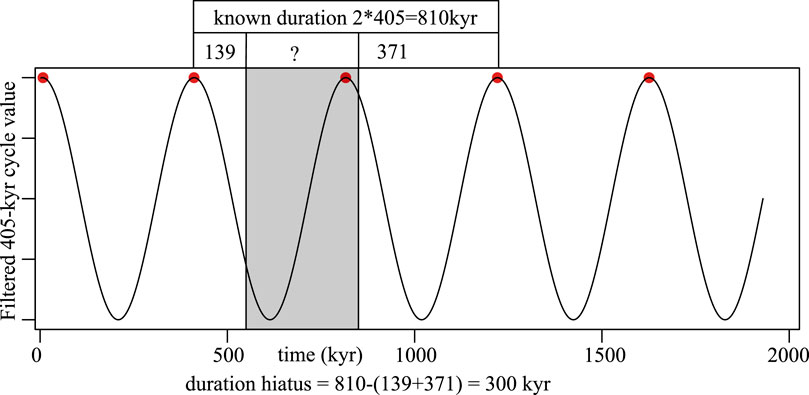
Figure 3. Example of calculating the duration of the hiatus (grey box) using the stable 405-kyr eccentricity cycle. The known interval between the last peak before and the first peak after the hiatus is 810 kyr (2 × 405 kyr). The duration between the last peak before the hiatus and the hiatus is 139 kyr. The duration between the hiatus and the first peak after is the hiatus 371 kyr. The duration of the hiatus is 810 (139 + 371) = 300 kyr.
The “dur_gaps” function of the WaverideR package utilises the rationale mentioned above to simulate the duration of the hiatus using a Monte Carlo simulation. The primary input parameters for the simulation are the outcomes of the “retrack_wt_MC” Monte Carlo simulation (a mean tracked period (m) curve and uncertainty for the tracked 405-kyr eccentricity cycle). In the input parameters, it should also be specified whether the duration of the gap needs to be calculated between 405-kyr eccentricity minima or maxima, the number of simulations, and the number of 405-kyr eccentricity cycles present between the last 405-kyr eccentricity peak or trough before a hiatus and the first 405-kyr eccentricity peak or trough after the hiatus. The number of 405-kyr eccentricity cycles used as input should be based on existing (external) age constraints. In the case of the Cellon section, there are no dated ash beds, so external age controls are needed to define the number of 405-kyr eccentricity cycles as input for the “dur_gaps” function. The two dated bentonite beds from Podolia, Ukraine, namely, the M12 and C6 bentonites, are used as external age controls for the Cellon section (Figure 4). The correlation between Podolia and the Cellon section is primarily based on the conodont zonation, with secondary support from the δ13Ccarb curves (Figure 4). The cosmopolitan nature of Silurian conodont zonation allows for the correlation of the conodont zones between the sites (Cramer et al., 2010, 2011). The C6 bentonite is located within the upper part of the Oz. crispa biozone in Podolia Ukraine. Any diachronic or correlation differences means that C6 bentonite could be present in the lower third of the Oz. eosteinhornensi s.l. biozone in the Cellon section zone (Figure 4). The M12 bentonite was deposited in the upper part of the P. siluricus zone, which in the Cellon section forms part of a hiatus and the interval just below the hiatus (Figure 4). The M12 bentonite (424.08 ± 0.53 Ma) and the C6 bentonite (422.91 ± 0.49 Ma) are separated by an average duration of 1.17 million years.
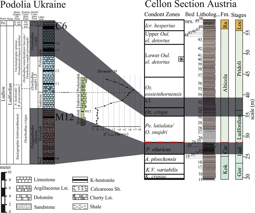
Figure 4. Correlation between the Podolia Ukraine composite of Cramer et al. (2015) (left) and the Cellon section in Austria (right). The δ13Ccarb peak in the Zhvanets 39 section corresponds to the δ13Ccarb peak of the Lau event. The correlation of the conodont zones is between the global conodont zones in the Podolia composite based on Cramer et al. (2011) and the conodont zonation of the Cellon section, which is based on Corradini et al. (2015). The * glyph indicates the Oz. eosteinhornensis s.s. horizon. Gor = Gorstian, Lud = Ludfordian, Loc = Lochkovian, Car = Cardiola and RK = Rauchkofel. The red line in the Cellon section indicates a hiatus.
According to Cramer et al. (2015), the Lau δ13Ccarb excursion encompasses roughly half of the stratigraphy between the M6 and M12 bentonites. The Cellon hiatus encompasses most of the Lau δ13Ccarb excursion and potentially extends into a brief period preceding the Lau δ13Ccarb excursion. This hiatus likely includes the timeframe during which the M12 bentonite was deposited. The Cellon section’s hiatus overlaps almost entirely with the interval between M6 and M12 bentonites. Therefore, it can be concluded that the maximum duration of the hiatus in the Cellon section does not exceed the duration between the M6 and M12 bentonites. Based on these age constraints, it is inferred that the “dur_gaps” function needs to be run with one and two 405-kyr eccentricity cycles present between the last minima/maxima before the hiatus and the first minima/maxima above the hiatus. Therefore, the “dur_gaps” function will run 10,000 simulations using one and two missing cycles as input. From these runs, it will be possible to calculate the mean duration of the hiatus and standard deviation.
3.2.2.5 Anchoring the data in the time domain
In the absence of dated ash beds in the Cellon section, the C6 bentonite from Podolia, Ukraine (422.91 ± 0.49 Ma U/Pb date) from Cramer et al. (2015) is transposed into the Cellon section using a Monte Carlo simulation. The Monte Carlo simulation is implemented using the “curve2time_unc_anchor” function of the WaverideR package. The Monte Carlo simulation starts by randomly (using a uniform distribution) selecting a position (m) within the Oz. crispa biozone and the lower third of the Oz. eosteinhornensi s.l. biozone in the Cellon section as the hypothetical location of the C6 bentonite (see Section 3.2.2.4 for the correlation). An anchoring age is then assigned to the hypothetical position of the C6 bentonites, which is randomly generated using a normal distribution based on the published age and uncertainty of the U/Pb date of the C6 bentonite. The age and location of the C6 bentonite, modelled in the Cellon sections, are used to anchor a floating age model. The floating age model is based on four inputs, which are the tracked period curve (m) with uncertainty for the 405-kyr eccentricity cycle from the “retrack_wt_MC” function for the intervals between 19.5 and 28.47 m and between 28.47 and 40.15 m, the tracked period of the 405-kyr eccentricity cycle with uncertainty based on the analytical uncertainty of the wavelet for the interval between 40.15 and 58.16 m and the duration and uncertainty for the hiatus 28.47 m generated using the “dur_gaps” function. These four results are combined in the Monte Carlo simulation, which (randomly) generates a new floating age-depth curve with a (randomly) generated duration for the hiatus, which is then anchored to the modelled location and age of the C6 bentonite. This time-anchored age curve is then used to convert a randomly selected proxy record to the absolute time domain. The randomly selected record is then checked for the imprint of astronomical cycles by examining whether the spectral peaks of the 100-kyr and 405-kyr eccentricity are present in the average spectral power spectra of CWT of the record. The detection range of the 100-kyr eccentricity cycle peak spans ±20 kyr, allowing it to span from the 125-kyr eccentricity cycle to the 95-kyr eccentricity cycle (Laskar et al., 2004). For the 405-kyr eccentricity, the detection range of the spectral peak was set at ±10% of the period of said cycle. This detection range is large enough to allow for variations in the duration of the 405-kyr eccentricity while excluding the spectral peaks of the 346-kyr and 486-kyr eccentricity cycles (Laskar et al., 2004). If spectral peaks belonging to the 100-kyr and 405-kyr eccentricity are observed, only then the depth-absolute time curves and generated hiatus durations are saved. The process is restarted if no astronomical cycles are detected until a valid curve is obtained. This process is repeated 10,000 times, resulting in a set of depth-age curves. The mean age and uncertainty for each stratigraphic position are calculated from these curves. The resulting absolute age-depth curve with uncertainty is then used to assign absolute ages and durations [with 2σ (∼95% percentile) uncertainty] to geological units, including conodont zones, chronostratigraphic/geochronologic units, lithological units, and events. Furthermore, the 10,000 saved hiatus durations are used to re-calculate the mean duration and uncertainty for the hiatus.
3.2.2.6 Astronomical imprint in the time domain
The CWT (“analyze_wavelet” function) using an omega number of 6 is performed on the data anchored in the time domain, allowing for the visualisation of the imprint of astronomical cycles on the proxy records. From the wavelet scalogram, the 405-kyr eccentricity, 100-kyr eccentricity, obliquity, and precession cycles are extracted using the “extract_signal_stable” function. The Hilbert transform (“hilbert” function of the Astrochron R package) is used to extract the amplitude modulation from the 100-kyr eccentricity, obliquity, and precession. Next, a CWT is performed on the Hilbert transform of the 100-kyr eccentricity cycle, from which the amplitude modulating (g2–g5) 405-kyr eccentricity and (g4–g3) 2.4-Myr eccentricity are extracted. It is especially preferable to extract the 2.4-Myr eccentricity cycle via the amplitude modulation rather than direct filtering due to the unstable nature of the 2.4-Myr eccentricity cycle caused by the chaotic behaviour of the Solar System (Laskar et al., 2004, 2011).
4 Results
4.1 Chemostratigraphic proxy trends in the Cellon section
Fe2O3 and Al2O3 are proxies for terrigenous input, while CaO indicates carbonate content, and induration reflects bed competence (Rothwell and Croudace, 2015). In the Cellon section, the induration pattern closely mirrors the CaO record, indicating that carbonate determines bed competence (Figure 2). The Fe2O3 and Al2O3 proxies are anti-phased with the CaO and induration, with higher Fe2O3 and Al2O3 values in shales/marls (Figure 2). The Kok Formation exhibits minimal proxy variation compared to the overlying Cardiola Formation. For instance, Fe2O3 values range from 0% to 5% in Kok and 0%–20% in Cardiola. The proxies remain stable in the 28.47–32.95 m interval of the Alticola Formation, which is attributed to dolomitisation, as evidenced by elevated MgO values (reaching 15%) and pervasive dolomitisation observed in thin sections (see Supplementary Material S4). The record of induration indicates a rise in variability within the middle section of the Alticola Formation and the transition into the Rauchkofel Formation. During this transition, the thickness of limestone beds decreased from decimetre to centimetre scale.
4.2 Visual recognition of cyclic bundles
The Kok and Cardiola Formations exhibit distinct cyclic bedding patterns, which can be preliminarily identified through visual analysis in the proxy record and an outcrop picture (Figure 5). Hierarchical bedding patterns are also observable in the Alticola and Rauchkofel Formations, albeit with a lower overall bundling quality (see Supplementary Material S1). The primary bedding is likely the result of astronomical cycles and sub-Milankovitch scale environmental cyclicity. The visual identification of the first, second, and third-order cycles (smallest to largest) will be used as a guide for interpreting the wavelet scalograms. It is important to note that the litholog of Walliser (1964) was not made to conduct a cyclostratigraphic analysis. Consequently, there are intervals where it is hard to resolve first-order cycles using the litholog (see Supplementary Material S1).
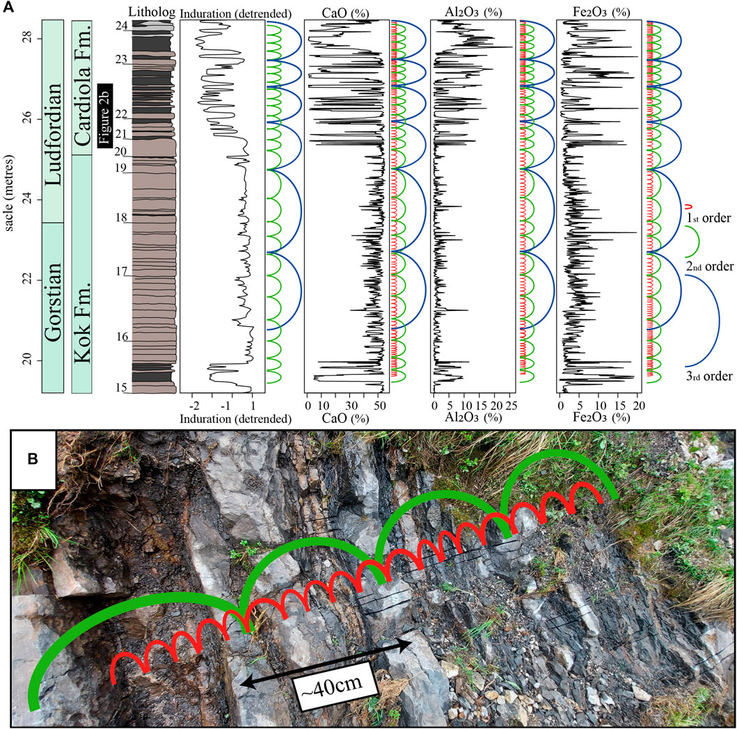
Figure 5. Visual identification of first, second and third-order cycles. (A) First-order cycles bundled in second- and third-order cycles were observed in the proxy records in the Kok and Cardiola Formations. From left to right, the columns indicate/are stage boundaries, Formations, litholog including bed numbers which were digitised after Walliser (1964), induration record, CaO, Al2O3, and Fe2O3. (B) First-order cycles (red) bundled in second cycles (green) were observed in the Cardiola Formation in the Cellon section between 25.19 and 26.88 m.
Within the Cellon section, an order of cycles can be observed (see Figure 5A; for an in-depth description per Formation, see Supplementary Material S1), with first-order cyclicity characterised by alternation between competent limestones and soft indurated shales/marls. The shales/marls have high Fe2O3 and Al2O3 values, while the limestone beds have high CaO values. On average, second-order cycles include six first-order cycles identified as changes from CaO-rich intervals with low lithological variation to intervals containing more indurated thin shales/marls and higher amplitude bed-to-bed variations and evaluated Fe2O3 and Al2O3 values. Third-order cycles include ∼3.5 second-order cycles and are identified as changes from intervals consisting primarily of carbonates with very low variations in indurations with no or only thin shales/marls being present to intervals with clear limestone-marls/shale alternations. It is worth noting that the thickness of the different order cycles changes in the section (see Figure 5A and Supplementary Material S1). The thickness of the first order cycle varies from approximately 0.3 m in the Kok and Cardiola Formations to around 1.5 m at the base of the Alticola Formation before decreasing to 0.8 m for the remainder of the Alticola Formation. Still, the ratio remains stable at 21:3.5:1, which is almost identical to the 19.2:110:405 (21:3.6:1) ratio between precession, 100-kyr eccentricity, and 405-kyr eccentricity calculated for the Silurian (Laskar et al., 2004; Waltham, 2015). The first, second, and third-order cycles are interpreted as precession, 100-kyr, and 405-kyr eccentricity. The Alticola and Rauchkofel Formations display the hierarchy of astronomical cycles, although, in some areas, the lithological differences are too small to observe first-order cycles (see Supplementary Material S1) clearly. The second-order cycles, interpreted as 100-kyr eccentricity, are the most pervasive in the record.
4.3 Age modelling using the WaverideR R package
4.3.1 Tracking the 405-kyr eccentricity cycle in wavelet scalograms
The visual identification of cycles and their respective thickness allowed to track the 405-kyr cycle in the wavelet scalogram of the Al2O3, Fe2O3, CaO and induration records. Two wavelet scalograms were created for each proxy record, one below the hiatus at 28.47 and one above (Figures 6, 7 and Supplementary Material S3), resulting in eight wavelet scalograms (see Figure 6 and Supplementary Material S3). Although the 100-kyr eccentricity is the most pervasive in the visual bundling observations, its composite nature hinders the construction of an astrochronology, and the highly stable 405-kyr eccentricity cycle is used instead to construct the astrochronology (Laskar et al., 2004, 2011).
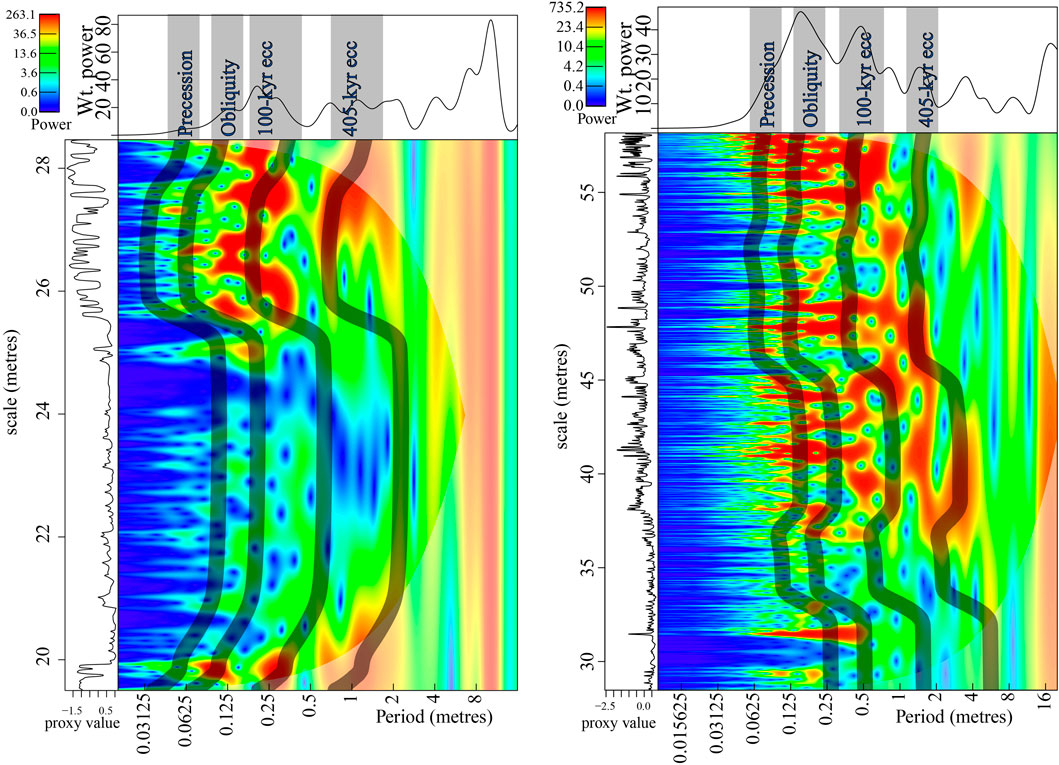
Figure 6. Wavelet scalograms of the induration records. The wavelet scalogram on the left spans the induration record between 19.5 and 28.47 m. The wavelet scalogram on the right spans the induration record between 28.47 and 58.16 m. The tracked period of the 405-kyr eccentricity cycle in the wavelet scalograms is recalculated using the ratios between the 405-kyr eccentricity cycle and the 100-kyr eccentricity, obliquity, and precession cycles and plotted in the depth domain to show that said astronomical tracking paths coincide with known astronomical cycles.
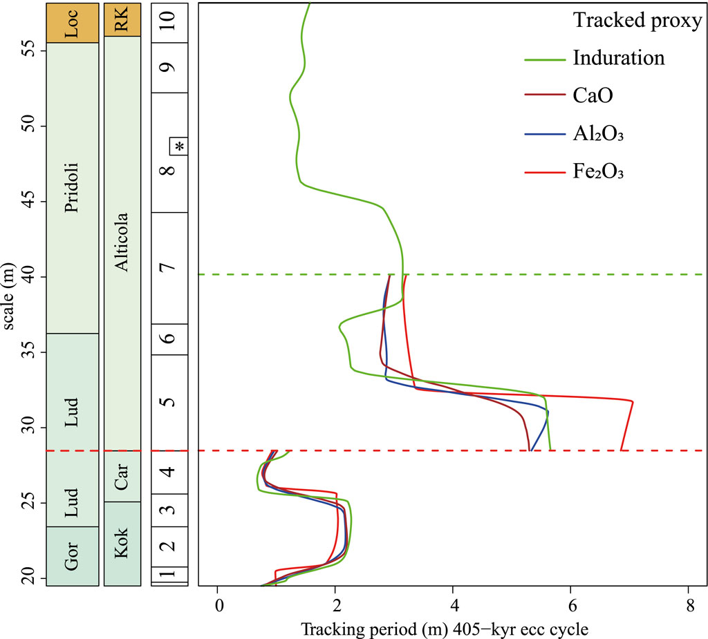
Figure 7. Tracked period (m) curve of the 405-kyr eccentricity cycle of the four proxy records. From left to right, stage boundaries (Gor = Gorstian, Lud = Ludfordian and Loc = Lochkovian), Formations (Car = Cardiola and RK = Rauchkofel), conodont zonation, and the results of tracking the period (m) of the 405-kyr eccentricity cycle in the wavelet scalogram. Numbers 1–10-* correspond to the conodont zones K. crassa (1)., K.v. variabilis (2), A. ploeckensis (3), P. siluricus (4), Pe. latialata/Oz. snajdri (5), Oz. crispa (6), Oz. eosteinhornensi s.l. (7), Lower Oul. el. detortus (8), Upper Oul. el. detortus (9) Icr. hesperius (10) and (*) Oz. eosteinhornensis s.s. horizon. The red dotted line indicates the hiatus at 28.47 m. The green dotted line at 40.15 indicates the end of the pXRF data.
To validate the tracked period of the 405-kyr eccentricity cycle, the phase relationship between the 405-kyr eccentricity cycle extracted from the proxy records and the 405-kyr eccentricity cycle extracted from the amplitude modulation of the 100-kyr eccentricity cycle was checked (see Section 3.2.2.1 for further explanation and Supplementary Material S2 for the phase relationships of the different proxies). An antiphase relationship can be observed for the CaO and induration records, and an in-phase relationship for the Al2O3 and Fe2O3 records (see Supplementary Material S2). The stability of the phase and the similarity in the tracked curves of the 405-kyr eccentricity cycle suggest that the period of the 405-kyr eccentricity cycle was consistently tracked across different proxy records, supporting the interpretation of the astronomical cycle’s imprint in the proxy records. The observed phase relationships also indicate that during an (orbital) eccentricity maximum, Fe2O3 and Al2O3 are high, whereas induration and CaO are low. This phase relationship can be explained by the fact that during an eccentricity, maxima seasonality increases, which leads to higher runoff, increasing detrital products (Fe2O3 and Al2O3) and decreasing carbonate productivity (induration and CaO) (Mutterlose and Ruffell, 1999; Martinez, 2018).
A second quality check was conducted on the tracked period of the 405-kyr eccentricity by verifying the alignment between the tracked period (m) curve of the 405-kyr eccentricity cycle and the spectral peaks of other known astronomical cycles (see Section 3.2.2.1). The tracked period (m) of the 405-kyr eccentricity cycle was recalculated using the ratios between the 405-kyr eccentricity cycle and the 100-kyr eccentricity, obliquity, and precession cycles (Laskar et al., 2004; Waltham, 2015). The resulting curves were plotted in the wavelet scalograms (Figure 6 and Supplementary Material S3). The tracked period (m) curves of precession, obliquity and short eccentricity track through high spectral power blob or sausage-shaped areas, confirming that the tracking of the 405-kyr eccentricity cycle was correct. The fact that the spectral power is not continuous in the tracks of the transposed cycles is due to the modulation of the spectral power by higher-order cycles. The lack of spectral power in the tracked (m) curves of the precession and obliquity cycles in the induration record (Figure 6) is due to the much lower sampling in density compared to the Al2O3, Fe2O3, and CaO proxy datasets, indicating that the resolution in the induration dataset is insufficient to resolve the imprint of precession and obliquity properly.
4.3.2 Integrating tracked record results
To mitigate any tracking errors and accurately capture the uncertainty in the age model, two Monte Carlo simulation(s) were conducted. One simulation was run for the interval below the hiatus (19.5–28.47 m) and one for the interval (28.47–40.15 m) above the hiatus (see section for the methodology Section 3.2.2.2). From the resulting 10,000 simulated tracked period (m) curves of the 405-kyr eccentricity cycle, a mean period (m) and standard deviation for tracking the period (m) of the 405-kyr eccentricity cycle was calculated (see the interval between 28.47 and 40.15 m in Figure 8). The resulting means tracked period (m) of the 405-kyr eccentricity cycles and its corresponding uncertainty vary. In the interval below the hiatus, the average uncertainty as a fraction of the frequency (1/m) of the tracked 405-kyr eccentricity cycle is 0.058 (5.8%), whereas the average uncertainty for the interval above the hiatus is 0.083 (8.3%)
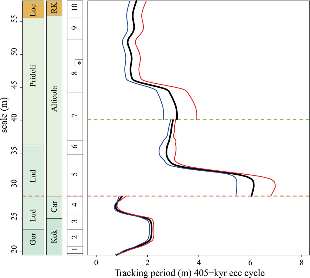
Figure 8. Tracked period (m) 405-kyr eccentricity cycle with uncertainty. From left to right, the columns indicate/are stage boundaries (Gor = Gorstian, Lud = Ludfordian and Loc = Lochkovian), Formations (Car = Cardiola and RK = Rauchkofel), conodont zonation, and tracked period (m) 405-kyr eccentricity cycle (black). The black line is the mean period (m) for the 405-kyr eccentricity cycle. The red and blue lines are the period (m) of the 405-kyr eccentricity cycle plus and minus one standard deviation (σ). The dotted line at 40.15 m indicates the end of the XRF. Below 40.15 m, the uncertainty is based on the “retrack_wt_MC” Monte Carlo simulations. Above 40.15 m, the uncertainty is based on the analytical uncertainty of the wavelet. Numbers 1–10 correspond to the conodont zones K. crassa (1)., K.v. variabilis (2), A. ploeckensis (3), P. siluricus (4), Pe. latialata/Oz. snajdri (5), Oz. crispa (6), Oz. eosteinhornensi s.l. (7), Lower Oul. el. detortus (8), Upper Oul. el. detortus (9) Icr. hesperius (10) and * indicates the Oz. eosteinhornensis s.s. horizon. The red dotted line at 28.47 m indicates a hiatus.
4.3.3 Assigning uncertainty using the analytical uncertainty of the wavelet
The induration record is the only proxy available for the interval between 40.15 m and 58.16. As such, it was impossible to generate a mean tracked period (m) of the 405-kyr eccentricity cycle and its uncertainty using the “retrack_wt_MC” Monte Carlo simulation. The wavelet’s analytical uncertainty utilising the “wavelet_uncertainty” function was used instead to assign one standard deviation of uncertainty to the tracking of the period (m) of the 405-kyr eccentricity cycle in the wavelet scalogram of the induration record between 40.15 m and 58.16 (see Section 3.2.2.3. for the methodology; Figure 8 for the results). The result is that a uniform fraction (0.13) (13%) of the frequency (1/m) of the tracked 405-kyr eccentricity cycle is used to assign the uncertainty. This uncertainty is higher than the average uncertainties from the “retrack_wt_MC” simulations.
4.3.4 Calculating the duration of the hiatus
To calculate the duration of the hiatus at 28.47 m, input based on the results from the Cellon section and input derived from external age controls were used (see Section 3.2.2.4 for the methodology). The output of the Monte Carlo simulations from which retracked the 405-kyr eccentricity cycle was used as the input for the age model (including uncertainty). The “dur_gaps” function also required the number of 405-kyr eccentricity cycles from the last peak/through before the hiatus to the first peak/through after the hiatus. In the case of Fe2O3 and Al2O3 records, the hiatus is calculated using the last pre-hiatus and the first post-hiatus 405-kyr eccentricity maxima. For induration and CaO records, the hiatus is calculated using the last pre-hiatus and the first post-hiatus 405-kyr eccentricity minima. Based on the external age constraints (see Section 3.2.2.4), one or two 405-kyr eccentricity cycles could be utilised as input. The “dur_gaps” function executed a total of 10,000 simulations using both one and two missing cycles as input. Using only one 405-kyr eccentricity cycle between the last peak/through before the hiatus and the first peak/through after the hiatus resulted in a negative duration estimation for the hiatus. Therefore, the result attained using two 405-kyr eccentricity cycles is the only valid result. The “dur_gaps” function produced a histogram with one large peak at 360 kyr and a smaller one at 600 kyr. The smaller amplitude mode at 600 kyr consists of outliers, which were removed using a cut-off value of 505 kyr (see Figure 9 for the histogram with the data points removed above the cut-off of 505 kyr). The duration of the hiatus, with the cut-off applied at 505 kyr, is 360 ± 95 (2σ) kyr.
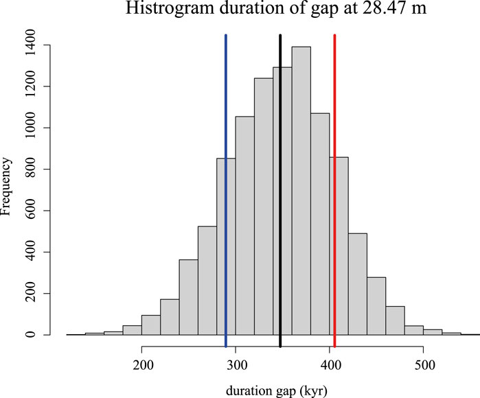
Figure 9. Histogram depicting the simulation results of modelling the duration of the hiatus at 28.47 m. Black line; mean duration of the hiatus (360 kyr). Blue line: duration of the hiatus minus one standard deviation (313 kyr). Red line: duration of the hiatus plus one standard deviation (407 kyr).
4.3.5 Converting the record into the absolute time domain
Direct radiometric dates are not available for the Cellon section; however, the existing conodont zonation allows for the modelling and transposition of the age (422.91 ± 0.49 Ma) of the C6 bentonite from Podolia, Ukraine, of Cramer et al. (2015), into the Cellon section (see Sections 3.2.2.4 and 3.2.2.5). The M12 bentonite of Cramer et al. (2015) cannot be used as a radiometric anchor because the bentonite was possibly deposited during a time interval, which coincides with a hiatus (28.47 m) in the Cellon section.
The “curve2time_unc_anchor” function, as described in Section 3.2.2.5, used the tracked 405-kyr eccentricity period (m) curves (including one standard deviation uncertainty), the modelled duration of the hiatus at 28.47 m (including one standard deviation uncertainty), the age and uncertainty of the C6 (422.91 ± 0.49 Myr) bentonite and the astronomical cycles and their uncertainty to be checked (405 ± 40.5 kyr and 110 ± 20 kyr) to generate absolute depth-time curves. The aggregate of the generated curves resulted in an absolute depth-time curve, including uncertainty for the Cellon section (Figure 10). The age model’s mean was used to convert the stage boundaries, Formations, conodont zonation, and proxy records to the absolute time domain (Figure 11). The depth-time curve, along with its uncertainty, is utilised to assign durations and ages, including their uncertainties, to the conodont zones, chronostratigraphic/geochronologic units, lithological units, and events in the Cellon section (Table 1; Figure 10) and those are discussed further in Section 5.2. The ages' uncertainties are given as two standard deviations (2σ) to align with the GTS (2020) (Goldman et al., 2020). All dates are rounded to the nearest ten thousand years to match the accuracy of the C6 bentonite, except for the Linde and Klev events, which are rounded to the nearest hundred thousand years due to their uncertain location.
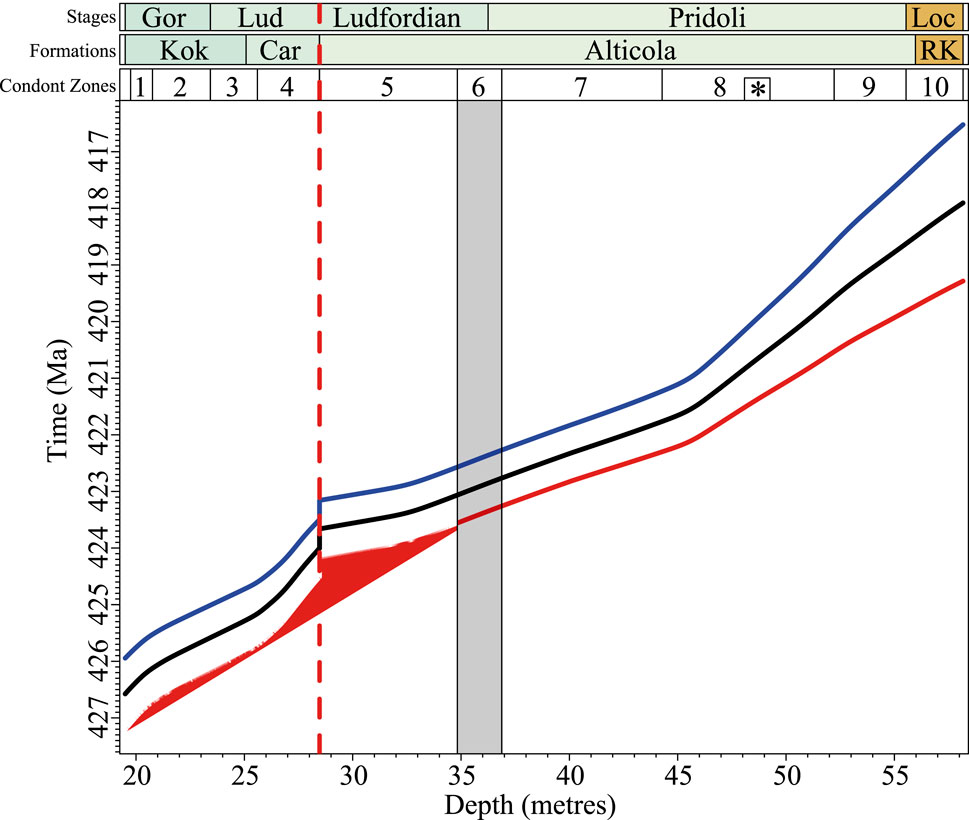
Figure 10. The absolute age model of the Cellon. The black line is the mean depth time curve, and the red and blue lines are time plus and minus two standard deviations (2σ), respectively. The red dotted line at 28.47 m indicates a hiatus. The grey box indicates the Oz. crispa biozone and the lower third of the Oz. eosteinhornensi s.l. in which the C6 bentonite was modelled. Numbers 1–10 correspond to the conodont zones K. crassa (1)., K.v. variabilis (2), A. ploeckensis (3), P. siluricus (4), Pe. latialata/Oz. snajdri (5), Oz. crispa (6), Oz. eosteinhornensi s.l. (7), Lower Oul. el. detortus (8), Upper Oul. el. detortus (9) Icr. hesperius (10) and * indicates the Oz. eosteinhornensis s.s. horizon. For the stages, Gor = Gorstian, Lud = Ludfordian and Loc = Lochkovian. For the Formations, Car = Cardiola and RK = Rauchkofel.
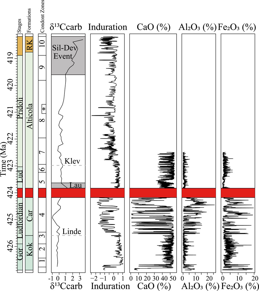
Figure 11. Data in the time domain. From left to right, the columns indicate/are stage boundaries (Gor = Gorstian, Lud = Ludfordian and Loc = Lochkovian), Formations (Car = Cardiola and RK = Rauchkofel) and conodont zonation; numbers 1–10 correspond to the conodont zones K. crassa (1)., K.v. variabilis (2), A. ploeckensis (3), P. siluricus (4), Pe. latialata/Oz. snajdri (5), Oz. crispa (6), Oz. eosteinhornensi s.l. (7), Lower Oul. el. detortus (8), Upper Oul. el. detortus (9) Icr. hesperius (10) and * indicates the Oz. eosteinhornensis s.s. horizon. The anchored and tuned δ13Ccarb, Induration, CaO (%), Al2O3(%), and Fe2O3 (%) records. The red box is a hiatus. The age scale is the mean anchored age in absolute time.
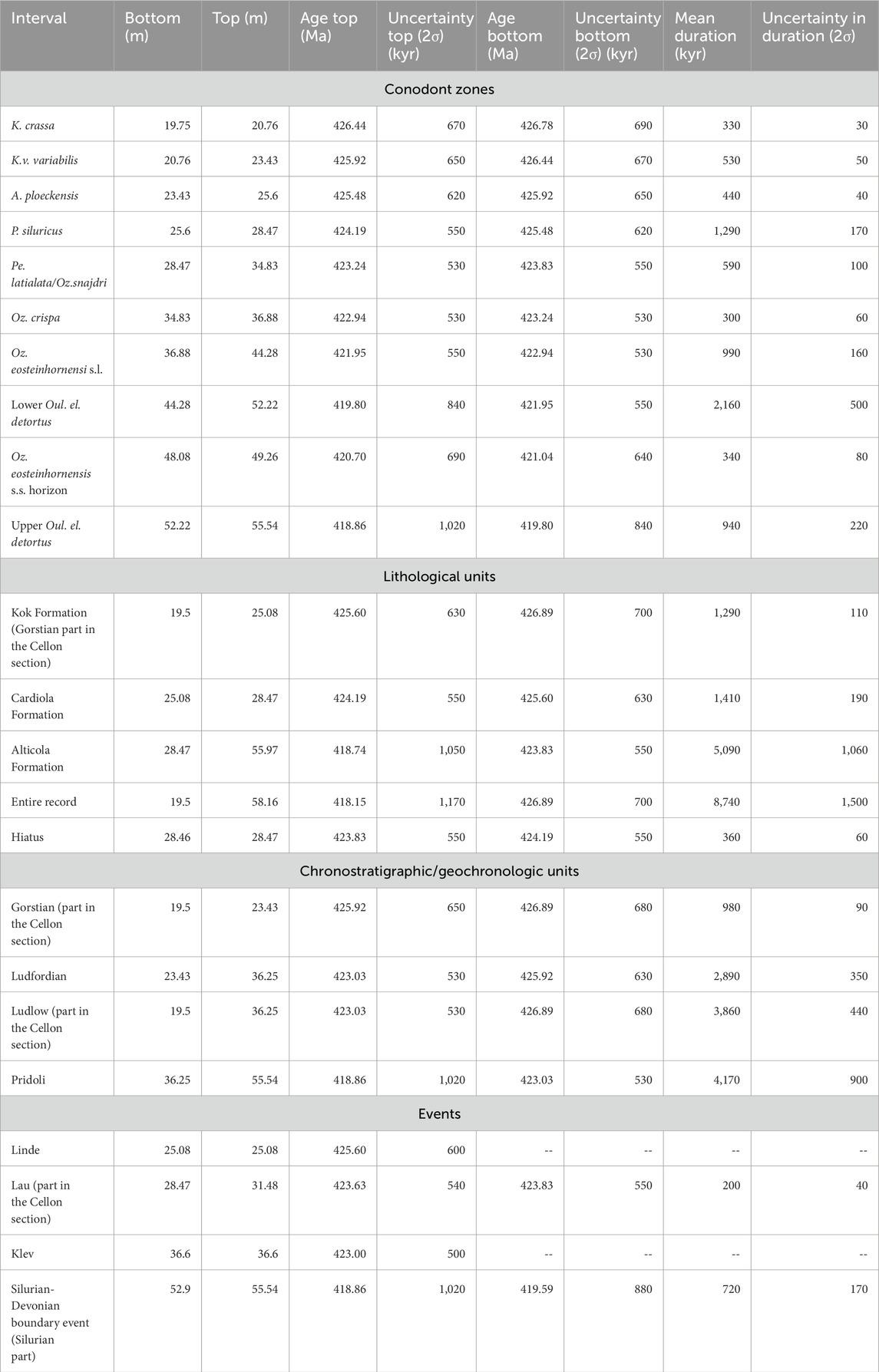
Table 1. Durations and ages for conodont zones, chronostratigraphic/geochronologic units, lithological units, and events. The Linde and Klev events have no durations due to poor stratigraphic constraints; therefore, only the mean age is given. The duration of the Lau event is the duration of the Lau event exposed in the Cellon section, excluding the duration of the hiatus. Ages for intervals with a top or bottom at 28.47 m are given up to the hiatus. All dates are rounded to the nearest 10 kyr to agree with the accuracy of the C6 bentonite, except for the Linde and Klev events, which are rounded to the nearest 100 kyr due to their uncertain location.
4.3.6 Spectral analysis and extraction of astronomical cycles in the time domain
To investigate the impact of astronomical forcing, specifically the 2.4-Myr eccentricity cycle, a continuous wavelet transform (CWT) was conducted on the proxy records, which were tuned using the mean absolute age model (Figure 12 and Supplementary Material S5). The 405-kyr eccentricity, 100-kyr eccentricity, precession, and obliquity cycles were extracted from the wavelet scalograms. The amplitude modulation of the 100-kyr eccentricity, precession, and obliquity was extracted from these cycles using the Hilbert transform. Subsequently, a CWT was conducted on the 100-kyr eccentricity amplitude record obtained from the Hilbert transform, enabling the extraction of the 405-kyr and 2.4-Myr eccentricity cycles. The results are plotted alongside the anchored data, lithological units, conodont zonation, and δ13Ccarb record (Figure 12 and Supplementary Material S5) and will be discussed further in Section 5.3. The results show that the Linde, Klev and Silurian-Devonian events occur just after a 2.4-Myr eccentricity minimum, whereas the Lau event occurs just before a minimum.
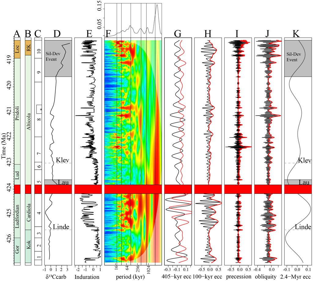
Figure 12. (A) Induration proxy record in the time domain including the wavelet scalogram of the induration record and astronomical cycles extracted from said record. The (A) stages (Gor=Gorstian, Lud = Ludfordian and Loc = Lochkovian). (B) Formation (RK = Rauchkofel), (C) conodont zonation, Numbers 1–10 correspond to the conodont zones K. crassa (1)., K.v. variabilis (2), A. ploeckensis (3), P. siluricus (4), Pe. latialata/Oz. snajdri (5), Oz. crispa (6), Oz. eosteinhornensi s.l. (7), Lower Oul. el. detortus (8), Upper Oul. el. detortus (9) Icr. hesperius (10) and * indicates the Oz. eosteinhornensis s.s. horizon. (D) The δ13Ccarb record. (E) The Induration record. (F) Wavelet scalogram of induration record with the average spectral power on top. The black vertical lines in the wavelet scalograms are durations of known astronomical cycles. From left to right, these cycles are the 19-kyr precession, 34-kyr obliquity, 100-kyr eccentricity, 405-kyr eccentricity, 800-kyr eccentricity and the 2.4-Myr eccentricity cycle. (G) The black line is a 405-kyr eccentricity cycle extracted from the Induration record. The red line is the 405-kyr eccentricity cycle extracted from the Hilbert transform of the 100-kyr eccentricity cycle of the Induration record. (H) The 100-kyr eccentricity cycle was extracted from the Induration record (black line) and the Hilbert transform of the 100-kyr eccentricity cycle (red line). (I) The precession cycle extracted from the Induration record (black line) and the Hilbert transform of the precession cycle (red line). (J) Obliquity cycle extracted from the Induration record (black line), and the Hilbert transform of the obliquity cycle (red line). (K) 2.4-Myr eccentricity cycle extracted from the Hilbert transform of the 100-kyr eccentricity cycle extracted from the Induration record. The red blocked time interval in the figure is the time interval encompassed by the hiatus at 28.47 m.
5 Discussion
5.1 Creating an astrochronology using the WaverideR package
Defining the uncertainties of the astrochronological models is an ongoing work of the cyclostratigraphic community (Meyers et al., 2012; Westerhold et al., 2012; Da Silva et al., 2013, 2020; De Vleeschouwer and Parnell, 2014; Sageman et al., 2014; Li et al., 2016; De Vleeschouwer et al., 2017; Sinnesael et al., 2019; Harrigan et al., 2022). This work leveraged the WaverideR package’s functions to conduct a six-step cyclostratigraphic study, resulting in an anchored astrochronology with uncertainty. The six-step approach as a whole or some steps separately can be used in other future cyclostratigraphic studies. Each step’s results have implications that need to be clarified to understand each step’s applicability, advantages, and limitations.
In step (1), two ways were used to validate the cyclostratigraphic interpretation by checking the phase of extracted cycles and the presence of spectral peaks in the wavelet scalogram. A similar check can be readily implemented with or without the WaverideR package, and such a phase check should be done to ensure a correct cyclostratigraphic interpretation (see Sinnesael et al. (2019) on the importance of validating an astronomical interpretation through amplitude modulation patterns). In steps (2) and (3), an uncertainty was calculated/modelled for the tracked period (m) curve(s) of the 405-kyr eccentricity cycle (see Sections 4.3.2. and 4.3.3). Using the analytical uncertainty of wavelet (step 3) to assign an uncertainty to the tracked period (m) curve of the 405-kyr eccentricity cycle resulted in a higher uncertainty when compared to the uncertainty obtained through multiproxy Monte Carlo retracking simulation (step 2). The difference in uncertainty highlights the weakness of relying on a single proxy, showing that it is recommended to use multiple proxies when conducting a cyclostratigraphic study when possible. In step (4), the stable nature of the 405-kyr eccentricity cycle duration was used in a Monte Carlo to calculate the duration of the gap at 28.47 m in the Cellon section. The calculation of the duration of the hiatus includes the uncertainty stemming from the quality of the recording of astronomical forcing in the proxy records both before and after the hiatus. As external age controls were available, it was possible to calculate the duration of the gap. Such constraints might not always be available, and as such, using cyclostratigraphic results to constrain the duration of a hiatus will remain an uncommon part of future cyclostratigraphic studies. In step (5), a Monte Carlo simulation was conducted to create an anchored astrochronological timescale. The Monte Carlo simulation also included a check on the preservation of astronomical cycles. Leveraging the preservation of astronomical cycles remains an underutilised parameter when integrating astrochronologies and radiometric date (Trayler et al., 2023). Therefore, the “curve2time_unc_anchor” function is a novel and very useful function when trying to combine astrochronology and radiometric dates. In step (6), the proxy data in the absolute time domain was analysed using the CWT, followed by the extraction of astronomical cycles from the tuned proxy records. Extracting astronomical cycles after tuning is key in cyclostratigraphy and should progressively allow to have a complete picture of long astronomical forcing through geological time.
5.2 Duration and ages of intervals and boundaries in the Cellon section
The anchored astrochronological age model was used to assign ages, durations, and associated uncertainties to conodont zones, chronostratigraphic/geochronologic units, lithological units, and events, which are tabulated in Table 1.
5.2.1 Conodont zones
The durations of Silurian conodont zones, originally derived from constrained optimisation (CONOP) results by Sadler et al. (2009), have become outdated due to the generation of new U/Pb dates for Silurian and the subsequent updates of the global conodont zonation framework since 2009 (Cramer et al., 2011, 2015). The durations of conodont zones proposed in this work are the most up-to-date and accurate. However, the duration of the conodont zones is based solely on the results from the Cellon section. Therefore, all ages and durations are local. This means that the effect of diachroneity and or paleobiogeographical differences needs to be considered when applying these ages and duration to other records. The following section compares the ages proposed in the most recent Geologic Time Scale (GTS (Melchin et al., 2020)) to those from this study.
5.2.2 Lithological and chronostratigraphic/geochronologic units
This study covers the Gorstian Kok Formation to the lowest Lochkovian Rauchkofel Formation. The Gorstian part of the Kok Formation in the Cellon section lasted 1,290 ± 110 kyr. The Cardiola and Alticola Formations lasted 1,410 ± 190 kyr and 5,090 ± 1,060 kyr, respectively. Formation boundaries are conformable, except for the Cardiola and Alticola boundaries, representing an unconformity spanning 360 ± 60 kyr.
In the Cellon section, the boundary between the Homerian and Gorstian stages is tentatively placed at 19.5 m. This is indicated by an unzoned shale/marl, which suggests a condensed interval or possible hiatus (Jaeger, 1975; Corradini et al., 2015). The observed decrease in sedimentation rate and increased duration of this time interval most likely does not cover the entirety of the missing conodont zones (K. ortus absidata and Oz. bohemica longa), leaving the boundary poorly constrained (see Figures 6, 7 and Supplementary Material S3). The age generated for the Homerian-Gorstian boundary is 426.89 ± 0.68 Ma, which should be considered the maximum age of Gorstian-aged deposits in the Cellon section rather than the actual boundary age. Similarly, the duration of the Gorstian in the Cellon section of 0.98 ± 0.09 Myr only represents the duration of the Gorstian in the Cellon section. Due to the problematic boundary placement, the age and duration of the Gorstian in the Cellon section cannot be irrefutably determined. The Wenlock-Ludlow boundary is equivalent to the Homerian-Gorstian boundary; therefore, the same problem exists with this boundary and with the duration of the Ludlow (3.86 ± 0.44 My) in the Cellon section. The GTS (2020) provides ages and durations without this problem, making it the preferred source for the Homerian-Gorstian boundary and durations of the Ludlow and Gorstian (Melchin et al., 2020).
The Ludfordian of the Cellon section contains a hiatus at 28.47 m, spanning the Upper P. siluricus and part of the lower Pe. latialata/Oz.snajdri zone (Corradini et al., 2015, 2022). The hiatus is calculated to have lasted 360 (±60) kyr and covers the time interval from 423.83 ± 0.55 to 424.19 ± 0.55 Ma. This study establishes a Gorstian-Ludfordian boundary age of 425.9 ± 0.68 and a Ludfordian duration of 2.89 ± 0.35 Myr. These values have reduced uncertainties compared to the GTS 2020 (0.68 Myr in this study vs 1.5 Myr in the GTS 2020 and 0.35 Myr in this study vs. 3.1 Myr in the GTS 2020) (Melchin et al., 2020).
The age for the Ludfordian-Pridoli boundary is 423.03 ±0.53 Ma, according to this study. The age for this boundary has a reduced uncertainty compared to the GTS 2020 (0.53 Myr in this study vs 1.6 Myr in the GTS) (Melchin et al., 2020). The cyclostratigraphic study by Spiridonov et al. (2020) is the most recent estimate of the duration of the Pridoli (4.30 ± 0.2 Myr). Spiridonov et al. (2020) used a single proxy, leading to the possibility of potential false-positive frequencies being identified as an astronomical cycle (Ma and Li, 2020). The duration of the Pridoli determined by Spiridonov et al. (2020, 4.30 ± 0.2 Myr) and in this study (4.17 ± 0.9 Myr) are in close agreement, and therefore, the durations (including uncertainty) are combined using the summation in quadrature method, resulting in a duration of 4.24 ± 0.46 Myr for the Pridoli (JCGM, 2008). The combined result’s uncertainty is larger than the original 0.2 Myr uncertainty of Spiridonov et al. (2020). This new uncertainty is more robust and accurate, while the residual uncertainty (precision) is better accounted for.
The GTS (2020) (Goldman et al., 2020; Gradstein et al., 2020; Melchin et al., 2020) calculated an age of 419.0 ± 1.8 Ma for the Pridoli-Devonian boundary, while Husson et al. (2016) calculated an age of 421.3 ± 1.2 Ma. Husson et al. (2016) arrived at this age by first stretching the carbon isotope record to create a visually good fit between the different records and then using this stretched record as a relative timescale to extrapolate the age of the dated ash beds. There are two major problems with the age model. First, stretching the records produces a δ13Ccarb peak in the Lochkovian that has not been observed in other studies. The second problem is that the stretching factors and the introduction of hiatuses are not justified from a sedimentological point of view. The result is an overestimation of the age of the Silurian-Devonian boundary. The cyclostratigraphic results of this study provide absolute durations for the stratigraphic intervals studied, resulting in a better-constrained age for the Silurian-Devonian boundary of 418.86 ± 1.02 Ma.
5.2.3 Silurian events
In addition to the major Lau and The Silurian-Devonian boundary events. The Ludlow-Pridoli interval in the Cellon section also contains Linde and Klev events at ∼36.4 and ∼24.3 m (Jeppsson and Aldridge, 2000; Histon, 2012a, 2012b). The Klev and Linde events are associated with small increases in δ13Ccarb in the Cellon section (+0.4‰, see Figures 11, 12 and Supplementary Material S5). The δ13Ccarb record in the Cellon section is of rather low resolution; therefore, it is inappropriate to assign exact ages, durations and uncertainties to these events; instead, the ages at the midpoint (m) of these events are given at 425.6 Ma for the Linde event and 423 Ma for the Klev event. The best current estimate for the duration of the Lau is based on Cramer et al. (2015), who inferred a duration of 500 kyr for Lau δ13Ccarb excursion. In the Cellon section, the onset of the Lau event occurs in the hiatus at 28.47 m. It is impossible to determine the fraction of time in the hiatus that belongs to the Lau event; as such, only a minimum duration of 560 ± 100 kyr can be given for the Lau event. According to this study’s age model, the δ13Ccarb excursion of the Lau event ended at 31.48 m, which has an age of 423.83 ± 0.55 Ma. The Lau event started during the hiatus at 28.47 m, which lasted from 424.19 ± 0.55 to 423.83 ± 0.55 Ma, giving maximum and minimum ages for the onset of the Lau event. Based on the anchored astrochronology, the Silurian-Devonian boundary event started at 419.59 ± 0.88 Ma, and the Silurian part of the event lasted 720 ±170 kyr.
5.3 The 2.4-Myr eccentricity cycle and its pacing of Silurian events
Of all the astronomical cycles observed in the records of the Cellon section, the 2.4-Myr eccentricity cycle appears to be the most important when it comes to the pacing of Silurian (anoxic) events with the Linde, Klev and Silurian-Devonian events occurring just after a 2.4-Myr eccentricity minimum, with only the Lau event being the exception occurring during the descending limb of a 2.4-Myr eccentricity maximum (see Figure 12 and Supplementary Material S5). Other observed astronomical cycles do not have major implications, such as the 2.4-Myr eccentricity cycle, and, as such, are discussed in Supplementary Material S6.
The 2.4-Myr astronomical eccentricity cycle was extracted from the amplitude modulation of the 100-kyr eccentricity cycle, ensuring that it is a modulation cycle that was extracted and not a multimillion-year tectonic trend (see Sections 3.2.2.6 and 4.3.6). In the Cellon section, the 2.4-Myr eccentricity cycle varies in duration between 2 Myr and 2.8 Myr (Figure 12). This range in duration is consistent with the current range estimates of the duration of this cycle (Laskar et al., 2004, 2011; Olsen et al., 2019).
The Linde, Lau, Klev and Silurian-Devonian events show a similar phase relationship with the 2.4-Myr eccentricity cycle, suggesting a pacing by astronomical forcing. The observed phase relationship is very similar to the phase relationship observed during the Upper Devonian Lower Kellwasser and during the Cretaceous Oceanic Anoxic Event 2 events (Mitchell et al., 2008; Batenburg et al., 2016; De Vleeschouwer et al., 2017; Da Silva et al., 2020; Martinez et al., 2023). The pacing of biogeochemical events by astronomical forcing has been attributed to the dampening of seasonal extremes during the 2.4-Myr eccentricity minima, reducing runoff and productivity. During the first 100-kyr or 405-kyr eccentricity maxima following the 2.4-Myr eccentricity minimum, seasonality increases, increasing runoff and productivity, inducing ocean anoxia and the onset of (black) shale deposition, enhancing carbon burial and increasing δ13C values (Batenburg et al., 2016; De Vleeschouwer et al., 2017; Da Silva et al., 2020). For some biogeochemical events, complementary processes are invoked as an additional factor that could have pushed the global ocean towards a tipping point after which astronomical forcing could have accelerated the onset and evolution of ocean anoxia (Batenburg et al., 2016; Martinez et al., 2023).
The link between the Linde and Klev events, mainly bioevents, and the 2.4-Myr eccentricity cycle could be because seasonal extremes are reduced during the 2.4-Myr eccentricity minimum preceding the events, resulting in stable environmental conditions that reduce turnover rates. In contrast, during the transition from a period of environmental stasis (the 2.4-Myr eccentricity minimum) to a more dynamic climate system, turnover rates (the 2.4-Myr eccentricity maximum) increase, resulting in a bioevent (Bennett, 1990; Jansson and Dynesius, 2002). The transition from a period of environmental stasis to a more dynamic climate system is indeed observed in the sedimentary record of the Cellon section (Figure 12). The Linde event is located at the transition between the Kok and Cardiola Formations and is associated with a lithological transition between the massively bedded limestones of the Kok Formation and the increasingly shaly alternation of limestones and shales of the Cardiola Formation. The Klev and Silurian-Devonian boundary events coincide with an interval of increased induration differences, indicating a more dynamic depositional environment.
The δ13Ccarb excursion of the Silurian-Devonian event has a much larger amplitude than that of the Linde and Klev events. Given the similar astronomical forcing phase of the 2.4-Myr eccentricity cycle, some other external forcing mechanism driving the climate system to a tipping point should have operated concurrently with the astronomical forcing. Trigger mechanisms for the Silurian-Devonian event that have been proposed include increased volcanism, increased floral diversity, increased weathering rates that remove CO2, or the effect of increased erosion from the Caledonian orogen (Małkowski and Racki, 2009; Racki et al., 2012).
Given that the Linde, Klev and Silurian-Devonian events appear to be paced by the 2.4-Myr eccentricity cycle, it would make sense that at least one bio(event) should follow each 2.4-Myr eccentricity cycle. If true, a bio-event should be present in the middle Pridoli of the Cellon section (Figure 12). Other studies have identified events in the middle of Pridoli (Kaljo et al., 1995; Žigaite et al., 2010; Lehnert et al., 2012; Vandenbroucke et al., 2015). It remains unclear whether all these events in the Middle Pridoli refer to the same event. In the Cellon section, variations in δ13Ccarb and δ18Ocarb isotope values have been noted (Wenzel, 1997). These variations are of low amplitude, which could be part of the background noise. The interval around the 2.4-Myr eccentricity minimum includes a changing nautiloid composition, a pelagic incursion and several regressive transgressive cycles, which could be the imprint of the mid-Pridoli event in the Cellon section (Histon, 2012b, 2012a). The reason for the muted imprint of the mid-Pridoli event could be the 4.5-Myr eccentricity cycle [θ = 2(g4 − g3) − (s4 − s3) frequency combination], which has been invoked as a cycle that may have paced the Silurian (Sproson, 2020). The phase of the 4.5-Myr eccentricity cycle may have dampened the 2.4-Myr minimum, resulting in a dampened mid-Pridoli event. The interval studied in the Cellon section is too short (8.74 ± 1.50 Myr) to accurately observe the 4.5-Myr eccentricity cycle. Thus, the role of the 4.5-Myr eccentricity cycle in modulating the 2.4-Myr eccentricity cycle remains tentative, leaving uncertainty about its involvement in pacing Silurian events.
The Lau event does not occur after the 2.4 Myr eccentricity minimum, which could be explained by the unique rapidity of the processes occurring during the event. In the Kosov section, Czech Republic, the onset of the Lau/Kozlowskii bioevent, which precedes the δ13C excursion of the Mid-Ludfordian Carbon Isotope Excursion (MLCIE), coincides with a delimited but prominent peak in trace element concentrations (Frýda et al., 2021b). The unusually high trace element values indicate a rapid incursion of anoxic waters into the shallow shelf environment. This incursion of anoxic waters is accompanied by an increase in δ13C [interpreted by Frýda et al. (2021a, 2021b) as an increase in PCO2] and a temporary deepening of the basin. The Lau/Kozlowskii bioevent and the rising limb of the MLCIE occur within a time frame of thousands to tens of thousands of years (Koz and Sobie, 2012; Frýda et al., 2021a, 2021b). The rapid environmental change suggests that an external process triggered the Lau/Kozlowskii bioevent and the onset of the MLCIE, independent of the phase of the 2.4-Myr eccentricity cycle.
6 Conclusion
The WaverideR package introduced in this paper utilised a multistep approach to bring new solutions and perspectives to cyclostratigraphic analysis. First, the importance of checking the amplitude modulation patterns for the validity of the cyclostratigraphic model is insisted upon (see also Sinnesael et al., 2019). A new methodology is also proposed in which Monte Carlo simulations and wavelet-based uncertainty are used to address an ongoing problem in astrochronology, which is the definition of the uncertainty associated with a cyclostratigraphic model. With the uncertainty of a cyclostratigraphic model estimated, it is demonstrated that it is key to use multiple proxies when conducting a cyclostratigraphic analysis, as relying on a single proxy leads to higher uncertainty.
A new methodology for estimating a hiatus’s duration (and associated uncertainty) when external age controls are available is also proposed. Then, all the results from the combined age model of multiple proxies, hiatus, and external age control are integrated into an anchored age model with uncertainties. This multistep approach was applied to the Cellon section to constrain durations and ages of the upper Silurian and provide insights into the role that astronomical forcing plays in pacing Silurian events. The anchored cyclostratigraphic model provides new reference ages for the following boundaries: Gorstian-Ludfordian (425.92 ± 0.65 Ma), Ludfordian-Pridoli (423.03 ± 0.53 Ma) and Silurian-Devonian (418.86 ± 1.02 Ma) and gave new durations for the Ludfordian (2.97 ± 0.35 Myr) and Pridoli (4.24 ± 0.46 Myr). The hiatus in the record has a duration of 360 ± 60 kyr. The astronomical cycles extracted from the anchored age model indicate that the Linde, Klev and Silurian-Devonian events all occurred after a 2.4-Myr eccentricity minimum, similar to the Devonian Lower Kellwasser anoxic event and the Cretaceous Anoxic Oceanic Event 2, indicating that astronomical forcing may have played a crucial role in pacing Silurian oceanic (anoxic) events.
Data availability statement
The original contributions presented in the study are included in the article/Supplementary Material, further inquiries can be directed to the corresponding author.
Author contributions
MA: Conceptualization, Data curation, Formal Analysis, Investigation, Methodology, Project administration, Resources, Software, Validation, Visualization, Writing–original draft, Writing–review and editing. CC: Validation, Writing–review and editing. MP: Writing–review and editing. DP: Formal Analysis, Writing–review and editing. A-CD: Data curation, Formal Analysis, Funding acquisition, Investigation, Supervision, Writing–review and editing.
Funding
The author(s) declare that financial support was received for the research, authorship, and/or publication of this article. The FNRS-PDR T.0051.19 grant supported MA. A-CD was supported by the “Conseil Universitaire de la recherche et la valorisation,” as well as “Subside Fédéral de la recherche” for financial support for the acquisition of the Portable XRF Bruker Tracer 5G, as well as National Science Foundation grant (J.0037.21, T.0037.22, and R.5541-J-F-B). CC was supported by the Italian Ministry of University and Research Project 2022ZH5RWP, PRIN 2022 “DEEP PAST”. The Swiss National Science Foundation supported DP with grant PZ00P2-193520.
Acknowledgments
MA is financially supported by the FNRS-PDR T.0051.19 grant. A-CD acknowledges the “Conseil Universitaire de la recherche et la valorisation,” as well as “Subside Fédéral de la recherche” for financial support for the acquisition of the Portable XRF Bruker Tracer 5G, as well as National Science Foundation grant (J.0037.21, T.0037.22, and R.5541-J-F-B). CC acknowledges the Italian Ministry of University and Research Project 2022ZH5RWP, PRIN 2022 “DEEP PAST.” DP acknowledges the Swiss National Science Foundation grant PZ00P2-193520.
Conflict of interest
The authors declare that the research was conducted in the absence of any commercial or financial relationships that could be construed as a potential conflict of interest.
Publisher’s note
All claims expressed in this article are solely those of the authors and do not necessarily represent those of their affiliated organizations, or those of the publisher, the editors and the reviewers. Any product that may be evaluated in this article, or claim that may be made by its manufacturer, is not guaranteed or endorsed by the publisher.
Supplementary material
The Supplementary Material for this article can be found online at: https://www.frontiersin.org/articles/10.3389/feart.2024.1357751/full#supplementary-material
References
Arts, M. (2023). WaverideR: extracting signals from wavelet spectra. Available at: https://cran.r-project.org/package=WaverideR.
Batenburg, S. J., De Vleeschouwer, D., Sprovieri, M., Hilgen, F. J., Gale, A. S., Singer, B. S., et al. (2016). Orbital control on the timing of oceanic anoxia in the Late Cretaceous. Clim. Past 12, 1995–2009. doi:10.5194/cp-12-1995-2016
Bennett, K. D. (1990). Milankovitch cycles and their effects on species in ecological and evolutionary time. Paleobiology 16, 11–21. doi:10.1017/S0094837300009684
Brett, C. E., Ferretti, A., Histon, K., and Schönlaub, H. P. (2009). Silurian sequence stratigraphy of the carnic Alps, Austria. Palaeogeogr. Palaeoclimatol. Palaeoecol. 279, 1–28. doi:10.1016/j.palaeo.2009.04.004
Brett, C. E., McLaughlin, P. I., Histon, K., Schindler, E., and Ferretti, A. (2012). Time-specific aspects of facies: state of the art, examples, and possible causes. Palaeogeogr. Palaeoclimatol. Palaeoecol. 367–368, 6–18. doi:10.1016/j.palaeo.2012.10.009
Calner, M. (2004). The Silurian of Gotland–Part I: review of the stratigraphic framework, event stratigraphy, and stable carbon and oxygen isotope development: Erlanger geologischen Abhandlungen. Available at: http://www.gzn.uni-erlangen.de/fileadmin/images/pal/pdf/Calner_et_al_04a_02.pdf.
Cooper, R. A., Sadler, P. M., Munnecke, A., and Crampton, J. S. (2014). Graptoloid evolutionary rates track ordovician-Silurian global climate change. Geol. Mag. 151, 349–364. doi:10.1017/S0016756813000198
Corradini, C., Corriga, M. G., Ferretti, A., and Schönlaub, H. P. (2017). The Cellon section: Berichte des Institutes für Erdwissenschaften v. 23. Graz, Autria: Karl-Franzens-Universität Graz, 262–270.
Corradini, C., Corriga, M. G., Männik, P., and Schönlaub, H. P. (2015). Revised conodont stratigraphy of the cellon section (silurian, carnic Alps). Lethaia 48, 56–71. doi:10.1111/let.12087
Corradini, C., Corriga, M. G., and Pondrelli, M. (2022). “On the age of the Cardiola Formation (silurian) in the carnic Alps (Austria and Italy),” in European Conodont Symposium (ECOS), Utrecht 2022 - Abstracts and Programme, Utrecht, the Netherlands, September 23, 2022.
Corradini, C., Corriga, M. G., Pondrelli, M., and Suttner, T. J. (2020). Conodonts across the silurian/devonian boundary in the carnic Alps (Austria and Italy). Palaeogeogr. Palaeoclimatol. Palaeoecol. 549, 109097. doi:10.1016/j.palaeo.2019.02.023
Corradini, C., and Pondrelli, M. (2021). The pre-Variscan sequence of the Carnic Alps (Italy-Austria). Geol. Field Trips Maps 13, 1–72. doi:10.3301/GFT.2021.05
Corriga, M. G., Corradini, C., Schönlaub, H. P., and Pondrelli, M. (2016). Lower lochkovian (lower devonian) conodonts from cellon section (carnic Alps, Austria). Bull. Geosciences 91, 261–270. doi:10.3140/bull.geosci.1594
Cramer, B. D., Brett, C. E., Melchin, M. J., Männik, P., Kleffner, M. A., Mclaughlin, P. I., et al. (2011). Revised correlation of Silurian Provincial Series of North America with global and regional chronostratigraphic units and δ 13 C carb chemostratigraphy. Lethaia 44, 185–202. doi:10.1111/j.1502-3931.2010.00234.x
Cramer, B. D., and Jarvis, I. (2020). “Carbon isotope stratigraphy,” in Geologic time scale 2020 (Amsterdam, Netherlands: Elsevier), 309–343. doi:10.1016/B978-0-12-824360-2.00011-5
Cramer, B. D., Loydell, D. K., Samtleben, C., Munnecke, A., Kaljo, D., Mannik, P., et al. (2010). Testing the limits of Paleozoic chronostratigraphic correlation via high-resolution (<500 k.y.) integrated conodont, graptolite, and carbon isotope (δ13Ccarb) biochemostratigraphy across the llandovery-Wenlock (Silurian) boundary: is a unified Phanerozoic. Bull. Geol. Soc. Am. 122, 1700–1716. doi:10.1130/B26602.1
Cramer, B. D., Schmitz, M. D., Huff, W. D., and Bergström, S. M. (2015). High-precision u–pb zircon age constraints on the duration of rapid biogeochemical events during the ludlow epoch (Silurian period). J. Geol. Soc. 172, 157–160. doi:10.1144/jgs2014-094
Da Silva, A. C., Sinnesael, M., Claeys, P., Davies, J. H. F. L., de Winter, N. J., Percival, L. M. E., et al. (2020). Anchoring the Late Devonian mass extinction in absolute time by integrating climatic controls and radio-isotopic dating. Sci. Rep. 10, 12. doi:10.1038/s41598-020-69097-6
Da Silva, A. C., Triantafyllou, A., and Delmelle, N. (2023). Portable x-ray fluorescence calibrations: workflow and guidelines for optimizing the analysis of geological samples. Chem. Geol. 623, 121395. doi:10.1016/j.chemgeo.2023.121395
Da Silva, A. C. A. C., De Vleeschouwer, D., Boulvain, F., Claeys, P., Fagel, N., Humblet, M., et al. (2013). Magnetic susceptibility as a high-resolution correlation tool and as a climatic proxy in Paleozoic rocks – merits and pitfalls: examples from the Devonian in Belgium. Mar. Petroleum Geol. 46, 173–189. doi:10.1016/j.marpetgeo.2013.06.012
De Vleeschouwer, D., Da Silva, A. C., Sinnesael, M., Chen, D., Day, J. E., Whalen, M. T., et al. (2017). Timing and pacing of the Late Devonian mass extinction event regulated by eccentricity and obliquity. Nat. Commun. 8, 1–11. doi:10.1038/s41467-017-02407-1
De Vleeschouwer, D., and Parnell, A. C. (2014). Reducing time-scale uncertainty for the devonian by integrating astrochronology and bayesian statistics. Geology 42, 491–494. doi:10.1130/G35618.1
Frýda, J., Lehnert, O., Frýdová, B., Farkaš, J., and Kubajko, M. (2021a). Carbon and sulfur cycling during the mid-Ludfordian anomaly and the linkage with the late Silurian Lau/Kozlowskii Bioevent. Palaeogeogr. Palaeoclimatol. Palaeoecol. 564, 110152. doi:10.1016/j.palaeo.2020.110152
Frýda, J., Lehnert, O., Joachimski, M. M., Männik, P., Kubajko, M., Mergl, M., et al. (2021b). The Mid-Ludfordian (late Silurian) Glaciation: a link with global changes in ocean chemistry and ecosystem overturns. Earth-Science Rev. 220, 103652. doi:10.1016/j.earscirev.2021.103652
Goldman, D., Sadler, P. M., Leslie, S. A., Melchin, M. J., Agterberg, F. P., and Gradstein, F. M. (2020). “Chapter 20 - the ordovician period,” in Geologic time scale 2020. Editors F. M. Gradstein, J. G. Ogg, M. D. Schmitz, and G. M. Ogg (Amsterdam, Netherlands: Elsevier), 631–694. doi:10.1016/B978-0-12-824360-2.00020-6
F. M. Gradstein, J. G. Ogg, M. D. Schmitz, and G. M. Ogg (2020). “Chapter 14 - geomathematics,” Geologic time scale 2020 (Amsterdam, Netherlands: Elsevier), 401–439. doi:10.1016/B978-0-12-824360-2.00014-0
Harrigan, C. O., Schmitz, M. D., Over, D. J., Trayler, R. B., and Davydov, V. I. (2022). Recalibrating the Devonian time scale: a new method for integrating radioisotopic and astrochronologic ages in a Bayesian framework. Bull. Geol. Soc. Am. 134, 1931–1948. doi:10.1130/B36128.1
Hinnov, L. A. (2013). Cyclostratigraphy and its revolutionizing applications in the earth and planetary sciences. Bull. Geol. Soc. Am. 125, 1703–1734. doi:10.1130/B30934.1
Hinnov, L. A. (2018). Cyclostratigraphy and astrochronology in 2018. Amsterdam, Netherlands: Elsevier Ltd, 1–80. doi:10.1016/bs.sats.2018.08.004
Hinnov, L. A. L. A., and Hilgen, F. J. (2012). Cyclostratigraphy and astrochronology: the geologic time scale, 63–83. doi:10.1016/B978-0-444-59425-9.00004-4
Histon, K. (2012a). Paleoenvironmental and temporal significance of variably colored Paleozoic orthoconic nautiloid cephalopod accumulations. Palaeogeogr. Palaeoclimatol. Palaeoecol. 367–368, 193–208. doi:10.1016/j.palaeo.2012.07.008
Histon, K. (2012b). The silurian nautiloid-bearing strata of the cellon section (carnic Alps, Austria): color variation related to events. Palaeogeogr. Palaeoclimatol. Palaeoecol. 367–368, 231–255. doi:10.1016/j.palaeo.2012.10.012
Huang, C. (2018). Astronomical time scale for the mesozoic. Amsterdam, Netherlands: Elsevier Ltd, 81–150. doi:10.1016/bs.sats.2018.08.005
Husson, J. M., Schoene, B., Bluher, S., and Maloof, A. C. (2016). Chemostratigraphic and U-Pb geochronologic constraints on carbon cycling across the Silurian-Devonian boundary. Earth Planet. Sci. Lett. 436, 108–120. doi:10.1016/j.epsl.2015.11.044
Jaeger, H. (1975). Die Graptolithenführung im Silur/Devon des Cellon-Profils (Karnische Alpen): Carinthia II, v. 165./85, p. S, 111–126.
Jaeger, H., and Schönlaub, H. P. (1980). Silur und Devon nördlich der Gundersheimer Alm in den Karnischen Alpen (Österreich): Carinthia II, v. 170/190 3 figs., 5 pls., Klagenfurt, 403–444.
Jansson, R., and Dynesius, M. (2002). The fate of clades in a world of recurrent climatic change: Milankovitch oscillations and evolution. Annu. Rev. Ecol. Syst. 33, 741–777. doi:10.1146/annurev.ecolsys.33.010802.150520
Jarochowska, E., Bremer, O., Yiu, A., Märss, T., Blom, H., Mörs, T., et al. (2021). Revision of thelodonts, acanthodians, conodonts, and the depositional environments in the Burgen outlier (Ludlow, Silurian) of Gotland v. 143. Sweden: Gff, 168–189. doi:10.1080/11035897.2021.1907441
Jeppsson, L., and Aldridge, R. J. (2000). Ludlow (late Silurian) oceanic episodes and events. J. Geol. Soc. 157, 1137–1148. doi:10.1144/jgs.157.6.1137
Kaljo, D., Boucot, A. J., Corfield, R. M., Le Herisse, A., Koren, T. N., Kříž, J., et al. (1995). “Silurian bioevents,” in Global events and event stratigraphy in the Phanerozoic. Editor O. H. Walliser (Berlin, Heidelberg: Springer-Verlag), 173–224. doi:10.1007/978-3-642-79634-0_10
Koz, W., and Sobie, K. (2012). Mid-Ludfordian coeval carbon isotope, natural gamma ray and magnetic susceptibility excursions in the Mielnik IG-1 borehole (Eastern Poland) — dustiness as a possible link between global climate and the Silurian carbon isotope record. Palaeogeogr. Palaeoclimatol. Palaeoecol. 341, 74–97. doi:10.1016/j.palaeo.2012.04.024
Laskar, J., Fienga, A., Gastineau, M., and Manche, H. (2011). La2010: a new orbital solution for the long-term motion of the Earth. Astronomy Astrophysics 532, A89. doi:10.1051/0004-6361/201116836
Laskar, J., Robutel, P., Joutel, F., Gastineau, M., Correia, a. C. M., and Levrard, B. (2004). A long-term numerical solution for the insolation quantities of the Earth. Astronomy Astrophysics 428, 261–285. doi:10.1051/0004-6361:20041335
Lehnert, O., Fryda, J., Joachimski, M., Meinhold, G., and Cap, P. (2012). A latest silurian supergreenhouse: the trigger for the Pridoli transgrediens extinction event: 34th international geological congress.
Li, M., Ogg, J., Zhang, Y., Huang, C., Hinnov, L., Chen, Z. Q., et al. (2016). Astronomical tuning of the end-permian extinction and the early triassic epoch of south China and Germany. Earth Planet. Sci. Lett. 441, 10–25. doi:10.1016/j.epsl.2016.02.017
Ma, C., and Li, M. (2020). Astronomical time scale of the Turonian constrained by multiple paleoclimate proxies. Geosci. Front. 11, 1345–1352. doi:10.1016/j.gsf.2020.01.013
Małkowski, K., and Racki, G. (2009). A global biogeochemical perturbation across the Silurian-Devonian boundary: ocean-continent-biosphere feedbacks. Palaeogeogr. Palaeoclimatol. Palaeoecol. 276, 244–254. doi:10.1016/j.palaeo.2009.03.010
Martinez, M. (2018). Mechanisms of preservation of the eccentricity and longer-term Milankovitch cycles in detrital supply and carbonate production in hemipelagic marl-limestone alternations. Stratigr. Timescales 3, 189–218. doi:10.1016/bs.sats.2018.08.002
Martinez, M., Aguirre-Urreta, B., Dera, G., Lescano, M., Omarini, J., Tunik, M., et al. (2023). Synchrony of carbon cycle fluctuations, volcanism and orbital forcing during the Early Cretaceous. Earth-Science Rev. 239, 104356. doi:10.1016/j.earscirev.2023.104356
McLaughlin, P. I., Bancroft, A. M., Brett, C. E., and Emsbo, P. (2018). The rise of pinnacle reefs: islands of diversity in seas of despair. GSA Field Guid. 51, 23–33. doi:10.1130/2018.0051(02
McLaughlin, P. I., Emsbo, P., Brett, C. E., Bancroft, A. M., Desrochers, A., and Vandenbroucke, T. R. A. (2019). The rise of pinnacle reefs: a step change in marine evolution triggered by perturbation of the global carbon cycle. Earth Planet. Sci. Lett. 515, 13–25. doi:10.1016/j.epsl.2019.02.039
Melchin, M. J., Sadler, P. M., and Cramer, B. D. (2020). “Chapter 21 - the Silurian period,” in Geologic time scale 2020 Editors F. M. Gradstein, J. G. Ogg, M. D. Schmitz, and G. M. Ogg (Amsterdam, Netherlands: Elsevier), 695–732. doi:10.1016/B978-0-12-824360-2.00021-8
Meyers, S. R. (2019). Cyclostratigraphy and the problem of astrochronologic testing. Earth-Science Rev. 190, 190–223. doi:10.1016/j.earscirev.2018.11.015
Meyers, S. R., Siewert, S. E., Singer, B. S., Sageman, B. B., Condon, D. J., Obradovich, J. D., et al. (2012). Intercalibration of radioisotopic and astrochronologic time scales for the Cenomanian-Turonian boundary interval, western interior Basin, USA. Geology 40, 7–10. doi:10.1130/G32261.1
Mitchell, R. N., Bice, D. M., Montanari, A., Cleaveland, L. C., Christianson, K. T., Coccioni, R., et al. (2008). Oceanic anoxic cycles? Orbital prelude to the Bonarelli Level (OAE 2). Earth Planet. Sci. Lett. 267, 1–16. doi:10.1016/j.epsl.2007.11.026
Morlet, J., Arens, G., Fourgeau, E., and Giard, D. (1982a). Wave propagation and sampling theory—Part II: sampling theory and complex waves. GEOPHYSICS 47, 222–236. doi:10.1190/1.1441329
Morlet, J., Arens, G., Fourgeau, E., and Giard, D. (1982b). Wave propagation and sampling theory - Part I. Complex signal and scattering in multilayered media. Geophysics 47, 203–221. doi:10.1190/1.1441328
Mutterlose, J., and Ruffell, A. (1999). Milankovitch-scale palaeoclimate changes in pale-dark bedding rhythms from the Early Cretaceous (Hauterivian and Barremian) of eastern England and northern Germany. Palaeogeogr. Palaeoclimatol. Palaeoecol. 154, 133–160. doi:10.1016/S0031-0182(99)00107-8
Olsen, P. E., Laskar, J., Kent, D. V., Kinney, S. T., Reynolds, D. J., Sha, J., et al. (2019). Mapping solar system chaos with the geological orrery. Proc. Natl. Acad. Sci. U. S. A. 166, 10664–10673. doi:10.1073/pnas.1813901116
Pondrelli, M., Corradini, C., Spalletta, C., Simonetto, L., Perri, M. C., Corriga, M. G., et al. (2020). Geological map and stratigraphic evolution of the central sector of the Carnic Alps (Austria-Italy): Italian. J. Geosciences 139, 469–484. doi:10.3301/IJG.2020.16
Racki, G., Baliński, A., Wrona, R., Małkowski, K., Drygant, D., and Szaniawski, H. (2012). Faunal dynamics across the silurian-devonian positive isotope excursions (δ13C, δ18O) in Podolia, Ukraine: comparative analysis of the ireviken and klonk events. Acta Palaeontol. Pol. 57, 795–832. doi:10.4202/app.2011.0206
Rothwell, R. G., and Croudace, I. W. (2015). Micro-XRF studies of sediment cores: micro-XRF studies of sediment cores: applications of a non-destructive tool for the. Environ. Sci. 17, 25–35. doi:10.1007/978-94-017-9849-5
Russell, B., and Han, J. (2016). Jean morlet and the continuous wavelet transform: morlet and the continuous wavelet transform. CREWES Res. Rep. 28, 1–15.
Sadler, P. M., Cooper, R. A., and Melchin, M. (2009). High-resolution, early Paleozoic (Ordovician-Silurian) time scales. Bull. Geol. Soc. Am. 121, 887–906. doi:10.1130/B26357.1
Sageman, B. B., Singer, B. S., Meyers, S. R., Siewert, S. E., Walaszczyk, I., Condon, D. J., et al. (2014). Integrating 40Ar/39Ar, U-Pb, and astronomical clocks in the cretaceous niobrara formation, western interior basin, USA. U. S. A. GSA Bull. 126, 956–973. doi:10.1130/B30929.1
Schönlaub, H. P. (1979). Das Paläozoikum in Österreich VerbreitungStratigraphie, Korrelation, Entwicklung und Paläogeographie nicht-metamorpher und metamorpher Abfolgen, 142.
Schönlaub, H. P. (1992). Stratigraphy, Biogeography and Paleoclimatology of the Alpine Paleozoic and its Implications for Plate Movements: Jahrbuch der Geologischen Bundesanstalt, v. 135, 381–418. Available at: http://opac.geologie.ac.at/ais312/dispatcher.aspx?action=detail&database=ChoiceFullCatalogue&priref=200020132.
Schönlaub, H. P., Kreutzer, L. H., and Joachimskia, M. M. (1994). Paleozoic boundary sections of the carnic Alps (southern Austria), in geochemical event markers in the phanerozoic. Abstracts and guidebook abstracts and guidebook. Erlanger Geol. abh., 77–103.
Scotese, C. R. (2021). An atlas of phanerozoic paleogeographic maps: the seas come in and the seas go out. Annu. Rev. Earth Planet. Sci. 49, 679–728. doi:10.1146/annurev-earth-081320-064052
Sinnesael, M., De Vleeschouwer, D., Zeeden, C., Batenburg, S. J., Da Silva, A. C., de Winter, N. J., et al. (2019). The Cyclostratigraphy Intercomparison Project (CIP): consistency, merits and pitfalls. Earth-Science Rev. 199, 102965. doi:10.1016/j.earscirev.2019.102965
Spiridonov, A., Stankevič, R., Gečas, T., Brazauskas, A., Kaminskas, D., Musteikis, P., et al. (2020). Ultra-high resolution multivariate record and multiscale causal analysis of Pridoli (late Silurian): implications for global stratigraphy, turnover events, and climate-biota interactions. Gondwana Res. 86, 222–249. doi:10.1016/j.gr.2020.05.015
Sproson, A. D. (2020). Pacing of the latest Ordovician and Silurian carbon cycle by a ∼4.5 Myr orbital cycle. Palaeogeogr. Palaeoclimatol. Palaeoecol. 540, 109543. doi:10.1016/j.palaeo.2019.109543
Torrence, C., and Compo, G. P. (1998). A practical guide to wavelet analysis. Bull. Am. meteorological Soc. 79, 61–78. doi:10.1175/1520-0477(1998)079<0061:APGTWA>2.0.CO;2
Trayler, R., Schmitz, M., Schmitz, M., Meyers, S. R., and Meyers, S. R. (2023). Bayesian integration of astrochronology and radioisotope geochronology. Geochronology, 1–29. doi:10.5194/gchron-2023-22
Vandenbroucke, T. R. A., Emsbo, P., Munnecke, A., Nuns, N., Duponchel, L., Lepot, K., et al. (2015). Metal-induced malformations in early Palaeozoic plankton are harbingers of mass extinction. Nat. Commun. 6, 7966–7967. doi:10.1038/ncomms8966
von Raumer, J. F., and Stampfli, G. M. (2008). The birth of the Rheic Ocean - early Palaeozoic subsidence patterns and subsequent tectonic plate scenarios. Tectonophysics 461, 9–20. doi:10.1016/j.tecto.2008.04.012
Walliser, O. H. (1964). Conodonten des Silurs: Abhandlungen des Hessischen Landesamtes für Bodenforschung zu Wiesbaden, v. 41, 1–106.
Waltham, D. (2015). Milankovitch Period uncertainties and their impact on cyclostratigraphy. J. Sediment. Res. 85, 990–998. doi:10.2110/jsr.2015.66
Wenzel, B. (1997). Isotopenstratigraphische Untersuchnungen an silurischen Abfolgen und deren paläozeanographische Interpretazion: Erlanger geologischen Abhandlungen, v. 129, 1–117.
Westerhold, T., Röhl, U., and Laskar, J. (2012). Time scale controversy: accurate orbital calibration of the early Paleogene. Geochem. Geophys. Geosystems 13, 1–19. doi:10.1029/2012GC004096
Wu, H., Fang, Q., Hinnov, L. A., Zhang, S., Yang, T., Shi, M., et al. (2023). Astronomical time scale for the paleozoic era. Earth-Science Rev. 244, 104510. doi:10.1016/j.earscirev.2023.104510
Keywords: Silurian, wavelet, Monte Carlo simulation, WaverideR package, 2.4-Myr eccentricity node, δ13C excursion
Citation: Arts M, Corradini C, Pondrelli M, Pas D and Da Silva A-C (2024) Age and orbital forcing in the upper Silurian Cellon section (Carnic Alps, Austria) uncovered using the WaverideR R package. Front. Earth Sci. 12:1357751. doi: 10.3389/feart.2024.1357751
Received: 18 December 2023; Accepted: 23 April 2024;
Published: 05 June 2024.
Edited by:
Ángel Puga-Bernabéu, University of Granada, SpainReviewed by:
Huaichun Wu, China University of Geosciences, ChinaSiding Jin, Chengdu University of Technology, China
Copyright © 2024 Arts, Corradini, Pondrelli, Pas and Da Silva. This is an open-access article distributed under the terms of the Creative Commons Attribution License (CC BY). The use, distribution or reproduction in other forums is permitted, provided the original author(s) and the copyright owner(s) are credited and that the original publication in this journal is cited, in accordance with accepted academic practice. No use, distribution or reproduction is permitted which does not comply with these terms.
*Correspondence: Michiel Arts, TWljaGllbC5hcnRzQHVsaWVnZS5iZQ==