 Michael Haugeneder
 Michael Lehning
 Océane Hames1,2
 Mahdi Jafari
 Dylan Reynolds
 Rebecca Mott
- 1Snow and atmosphere, WSL Institute for Snow and Avalanche Research SLF, Davos, Switzerland
- 2Laboratory of Cryospheric Sciences, School of Architecture, Civil and Environmental Engineering, Ecole Polytechnique Fédérale de Lausanne, Lausanne, Switzerland
The near-surface boundary layer over patchy snow is highly heterogeneous and dynamic. Layers of opposing stability coexist within only a few horizontal meters. Conventional experimental methods to investigate this layer suffer from limitations related to the fixed positions of eddy covariance sensors. To overcome these difficulties, we set up a centimeter-resolution large eddy simulation of flow across an idealised transition from bare ground to snow. We force the simulation with high-frequency eddy covariance data recorded during a field campaign. We show that the model can represent the real flow by comparing it to independent eddy covariance data. However, the simulation underestimates vertical wind speed fluctuations, especially at high frequencies. Sensitivity analyses show that this is influenced by grid resolution and surface roughness representation but not much by subgrid-scale parameterization. Nevertheless, the model can reproduce the experimentally observed plumes of warm air intermittently detaching from bare ground and being advected over snow. This process is highly dynamic, with time scales of only a few seconds. We can show that the growth of a stable internal boundary layer adjacent to the snow surface can be approximated by a power law. With low wind speeds, deeper stable layers develop, while strong wind speeds limit the growth. Even close to the surface, the buoyancy fluxes are heterogeneous and driven by terrain variations, which also induce the frequent decoupling of a thin layer adjacent to the snow surface. Our simulations point the path towards generalizing point-based and aerial measurements to three dimensions.
1 Introduction
In spring, the snow that has accumulated throughout the winter begins to melt. The resulting run-off plays a crucial role, for example, for the ecosystem (Groffman et al., 2001; Wipf and Rixen, 2010; Wheeler et al., 2016; Rixen et al., 2022), drinking water supply (Sturm et al., 2017; Siirila-Woodburn et al., 2021), or hydropower generation (Stucchi et al., 2019; Magnusson et al., 2020). Furthermore, in combination with precipitation, it can amplify the risk of flooding and associated damages (Sui and Koehler, 2001; Würzer et al., 2016; Li et al., 2019; Mott et al., 2023), underscoring the necessity for a precise understanding and prediction of snowmelt dynamics.
The mountain snow cover is heterogeneous on a wide range of scales shaped by accumulation and ablation processes. Preferential deposition (Lehning et al., 2008), wind-induced snow transport (Föhn and Meister, 1983; Pomeroy and Gray, 1995), and avalanches lead to spatially varying snow depth (Quéno et al., 2023; Reynolds et al., 2024). These spatially irregular accumulation features, together with spatially heterogeneous melt, support the formation of patchy snow covers later in spring. Due to its lower albedo, the bare ground heats up faster than adjacent snow patches. In numerical simulations, studies by Ménard et al. (2014), Letcher and Minder (2017), and Schlögl et al. (2018a) demonstrated the resulting warming feedback for the near-surface atmosphere. The surface temperature of the snow is constrained by its melting temperature of 0°C. Consequently, there is a strong horizontal heat flux divergence between positive heat fluxes above bare ground and negative heat fluxes over snow-covered areas (Mott et al., 2015; Schlögl et al., 2018a).
Local-scale winds, influenced by small-scale surface temperature variations (Johnson et al., 1984) interact with larger-scale circulations such as valley breezes. The valley breeze, in turn, is influenced by an elevation gradient in snow cover: Lower parts of the valley are already snow-free, while higher up, the snow cover is still continuous (Farina and Zardi, 2023). The resulting winds mix the heterogeneously stratified air masses above the patchy snow cover. Warm air from bare ground is advected over snow-covered areas, leading to a strongly stratified layering. Close to the snow surface, a stable internal boundary layer (SIBL) forms (Garratt, 1990). A change in sign of sensible heat fluxes defines its upper boundary. Within the SIBL, negative (downward) fluxes prevail, while above it, positive (upward) fluxes align with the locally unstable stratification. The depth of the SIBL fluctuates rapidly depending on various parameters such as wind speed or stability (Mott et al., 2013; Schlögl et al., 2018a). In a recent experimental study, Haugeneder et al. (2024) examined the growth of a SIBL adjacent to a snow patch over a 3 week period of melt out. They observed that the depth of the SIBL decreased as the snow cover fraction diminished. Additionally, they noted that warm air plumes were intermittently advected over the snow surface, limiting the growth of the SIBL. These intermittent advections occurred on timescales of only a few seconds and only affected the lowest 1 m of the atmosphere adjacent to the snow surface. Thus, the feedback loops between heterogeneous surfaces in spring, the near-surface atmosphere, and the snow-atmosphere interaction processes are highly complex. Further experimental studies are essential for a comprehensive understanding and the development of valid parameterizations for models.
Experimentally investigating the atmosphere close to the surface poses some difficulties. Conventional eddy covariance (EC) measurements are limited to fixed positions and can not be deployed arbitrarily close to the surface (Stiperski and Rotach, 2016). Granger et al. (2006) performed temperature profile measurements at several positions across the transition from bare ground to snow using fine-wire thermocouples. However, this setup can also only sample data at limited locations. Recently, Haugeneder et al. (2023) adapted an approach from Grudzielanek and Cermak (2015) that allows aerial estimations of air temperature and wind speed close to the surface. In this technique, a thermal infrared camera pointing to thin vertically deployed synthetic screens records frames at 30 Hz. Since the screens have a low heat capacity, their surface temperature can be used as a proxy for the local air temperature. The measurements offer a spatial resolution of 0.5 cm and give insights into the dynamics of the near-surface atmospheric layer. However, they represent only snapshots in time and are confined to small measurement domains. Obtaining a comprehensive understanding of spatial dynamics solely from such measurements is challenging.
High-resolution numerical simulations offer the possibility to bridge the gap between point or aerial measurements and a full three-dimensional representation of the flow across the transition from bare ground to snow. The basis of most fluid dynamics simulations is the Navier-Stokes equations. The coupled system of partial differential equations describes and predicts the three-dimensional momentum field. A common technique to solve the coupled system is the Reynolds-averaged Navier-Stokes (RANS) approach. The Navier-Stokes equations are solved in RANS for time-averaged quantities, and turbulent motions of higher frequencies are parameterized. Due to its computational efficiency, it is used for modeling studies of the ABL (e.g., Balogh et al., 2012; Hames et al., 2022). It has also been used to study atmosphere-cryosphere interactions (Hames et al., 2022; Jafari et al., 2022). Challenges arise when the focus of the research is on turbulent quantities. Naturally, turbulence is not steady-state but transient. Therefore, only looking at time-averaged quantities does not yield enough information.
On the opposite side of the complexity spectrum for solving fluid dynamics problems is direct numerical simulation (DNS) (Pope, 2000). The Navier-Stokes equations can be accurately solved in idealized scenarios with relatively moderate Reynolds numbers. Eddies of all scales are directly resolved, and therefore no turbulence parameterization is necessary. For example, van der Valk et al. (2022) use a DNS model to simulate the near-surface boundary layer over patchy snow. Using temperature profile measurements above patchy snow from Harder et al. (2017), they found spatial variability in sensible heat fluxes that result in spatially heterogeneous melt rates. However, this computationally costly approach is limited to highly idealized conditions.
Large Eddy Simulations (LES) act as a robust intermediary, filling the complexity gap between RANS and DNS. By spatially filtering the Navier-Stokes equations, LES directly represents supra-filter scale motions while parameterizing sub-filter motions (Pope, 2000). Relevant energy-containing scales are directly resolved by choosing a suitable filter scale. In recent decades, multiple studies have applied the LES approach to study ABLs of various stability on a wide range of scales. Some more recent studies include Huang and Bou-Zeid (2013); Richardson et al. (2013); Zwaaftink et al. (2014); Smith and Porté-Agel (2014); Sigmund et al. (2022); Melo et al. (2024); Zahn and Bou-Zeid (2024). The review of Stoll et al. (2020) provides a comprehensive overview of studies.
In this work, we set up, validate, and analyze an LES simulation to study the near-surface atmosphere adjacent to the transition from bare ground to snow. Ultimately, we aim to generalize data recorded during a previous field campaign to get more information on the fetch dependence of heat fluxes close to the surface. Therefore, Sect. 2 gives an overview of the experimental data and the setup of the model followed by a validation of the model results with measurements in Sect. 3. In Sect. 4 we use the simulation results to investigate the near-surface boundary layer dynamics. Specifically, we examine the intermittent advection of plumes of warm air over the snow and the spatial and temporal dynamics of the SIBL. Furthermore, in Sect. 4.3 we analyze the dependence of vertical profiles of temperature and wind speed, as well as the SIBL depth, on wind speed. Section 5 summarizes the findings and gives a brief outlook.
2 Methods
2.1 Study site
In late spring 2021, we collected data during a comprehensive field campaign in the Dischma valley near Davos (Switzerland). The valley axis of the straight high alpine valley is oriented in the southeast-northwest direction. Steep slopes enclose the valley floor with an elevation difference of approximately 1000 m. The area has been extensively studied (Urfer-Henneberger, 1970; Lehning et al., 2006; Bavay et al., 2009; Brauchli et al., 2017; Wever et al., 2017; Mott et al., 2017; Schlögl et al., 2018a; b; Gerber et al., 2019; Carletti et al., 2022; Reynolds et al., 2023). Dürrboden, the flat measurement site at an elevation of
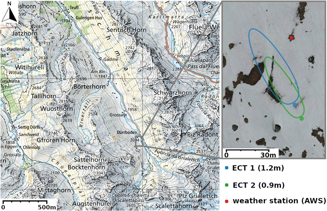
Figure 1. Topographic map of the Dischma valley end close to Davos (Switzerland). The coordinates of the bottom right corner of the map extent in the CH
To force and validate the LES simulation presented in this study, we use eddy covariance (EC) data recorded during this campaign. We deployed multiple sensors at various locations and heights. We installed two IRGASONs (Campbell Scientific, Logan, Utah, United States) on ECT1 at 1.2 m above the surface and on ECT2 at 0.9 m above the surface. Furthermore, at ECT2, we installed two CSAT3Bs (Campbell Scientific, Logan, Utah, United States) at heights of 1.9 and 2.9 m, together with a Campbell PT1000 ventilated air temperature sensor (Campbell Scientific, Logan, Utah, United States) positioned at 1 m above the surface. All EC sensors recorded data at a sampling frequency of 20 Hz. The lines in the UAV image indicate the
In addition to conventional EC measurements, we deployed thin synthetic screens vertically positioned across the transition from bare ground to snow. Using a thermal infrared camera to film these screens, we obtained surface temperatures at a spatial resolution of 0.6 cm and a temporal resolution of
2.2 Large eddy simulation
This study aims to set up, validate, and analyze a high-resolution numerical simulation of atmospheric flow over a single bare ground to snow transition forced with measurement data collected as described above. Therefore, we employ a large-eddy simulation (LES). LESs were first introduced in 1963 by Smagorinski (1963). Since then, the approach has grown rapidly and has become a popular and powerful tool to investigate atmospheric processes on various scales (Stoll et al., 2020).
In the following, we quickly summarize the basic concept and equations, which are important for the interpretation of the later results. For easier notation, we use the Einstein summation convention, in which a summation over the three spatial directions
The Navier-Stokes equations for incompressible flow predict the three-component velocity field
Directly solving Equation 1 and the incompressible continuity equation
is known as Direct Numerical Simulation (DNS). Due to the tremendous computational costs, this is (to date) only possible for highly idealized conditions. To reduce the computational demands, Equation 1 can be filtered. The filter, which can take on various shapes such as spectral cut-off or Gaussian, separates resolved large-scale motions from non-resolved and thus parameterized subgrid-scale (SGS) motions. This filtering step is the cornerstone of LES modelling. In our case, filtering is achieved implicitly by discretizing the mesh (Lund, 2003). We give a more detailed description of the model setup in Sect. 2.3. The filtered Equation 1 are
where variables with an overbar denote filtered quantities. The second term presents a challenge:
The Smagorinski-Lilly SGS model utilizes the concept of viscosity and builds upon the presence of an inertial subrange (Stoll et al., 2020). Within the frequency range of the inertial subrange, turbulent energy is transferred, in the mean, only from larger to smaller scales (Kolmogorov, 1941). If the filter is chosen to be in the inertial subrange, Smagorinski (1963) hypothesize a linear relation between the anisotropic residual stress and the filtered rate of strain
where
describes the eddy viscosity,
2.3 Model setup and forcing
We set up the LES simulation across an idealized transition from bare ground to snow. The computational domain spans
To allow for forcing with high-frequency EC measurements, we use inflow-outflow boundary conditions in the
The transition between bare ground and snow in the model at
We force the simulation directly with high-frequency EC measurements. To our knowledge, this has not yet been done in such a setup. Figure 2 gives an overview of the domain in relation to the available EC sensors. We chose the location of the domain such that the flow resembles the data captured by the IR screen setup. The idea is to apply the larger scale forcing via measured wind speeds and air temperatures and let the model simulate the surface-driven buoyancy effects at the transition from bare ground to snow.
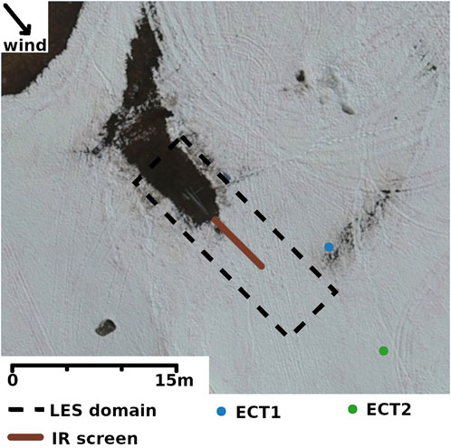
Figure 2. Location of the LES simulation domain (dashed black box) in relation to the measurement locations. The UAV image is a cutout from the one in Figure 1.
For wind speed forcing, we fit a logarithmic wind profile (log profile) through the median of 5 min EC data from three sensors at ECT2, which is the only location featuring multiple EC sensors at different heights. In the measurements, we do not see much difference between wind speed data recorded at ECT1 and ECT2 (apart from a time lag). Therefore, we assume that data from ECT2 sufficiently describes the flow structure at the inflow. To obtain a high-frequency wind profile, we scaled the log profile to the data measured at 0.9 m above the surface at ECT2.
A challenging task in LES modelling is to obtain realistic turbulence at the inlet. We use the divergence-free synthetic eddy method (DFSEM) developed by Poletto et al. (2013). The method generates realistically shaped eddies according to a given mean wind speed, Reynolds stress tensor, and turbulence integral length scale. We use 20 Hz horizontal wind speed data and calculated the Reynolds stress tensor from the 0.9 m EC sensor at ECT2. We also estimate the turbulence length scale from an auto-correlation analysis of this data. Additionally, we assume that the Reynolds stress tensor and the turbulence length scale are constant in the horizontal and vertical directions.
We do not apply vertical wind speed forcing, since we do not have enough measurement data to realistically interpolate, accounting for larger-scale vertical motions. However, the turbulent part of the vertical wind speed is generated by the DFSEM.
For temperature forcing, we use the upwind measurement at the AWS at 3.7 m height (see Figure 1). Since the AWS recorded data only every 10 min, we use the 5 s variations recorded by the ventilated thermometer at ECT2 scaled to the mean temperature measured at the AWS. We then logarithmically scale the air temperature to the surface temperature of bare ground of 15°C (Högström, 1996).
For the analysis in this study, we extract data on a slice aligned with the wind direction at
For the simulation, we use the buoyantBoussinesqPimpleFoam solver (OpenFoam API Guide, 2024) available from the open-source fluid dynamics platform OpenFOAM (Weller et al., 1998). The transient solver is designed for incompressible flow. OpenFOAM uses a finite volume method for discretization.
3 Validation of model results against measurements
In this section, our objective is to compare the LES simulation results with eddy covariance (EC) measurements. Therefore, we use the EC measurement at 1.2 m height on the ECT1. This particular EC measurement, not included in the initial model forcing, serves as an independent means of validation. Extracting data from the simulation domain at
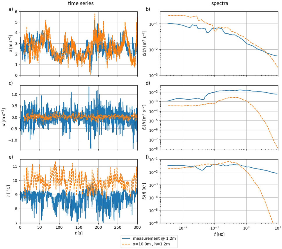
Figure 3. Comparison of model output at
The time series of wind speed along the flow presented in Figure 3 agree very well in both the absolute magnitude and the magnitude of the fluctuations. Nevertheless, a slight lag is observed between the two time series. This lag can be attributed to the setup depicted in Figure 1. Data for driving the LES simulations originate from ECT2, whereas the comparison data are obtained from ECT1 approximately 10 m upwind of ECT2. Consequently, the simulation exhibits a lag relative to the measurements. Nonetheless, the good agreement between measurement and simulation is also reflected by the spectra in Figure 3B. Both measurement and simulation agree well on all time scales. Time series and spectra indicate that the LES simulation features a realistic along-stream wind speed.
Furthermore, the mean vertical wind speed of the LES simulation at the extracted point
For the comparison of air temperature in Figure 3E, we corrected the measured sonic temperature with the simultaneously measured humidity according to Schotanus et al. (1983). The spectra presented in Figure 3F indicate a similar mismatch between the EC measurement and the simulation for
In summary, the LES simulation demonstrates remarkable capability in replicating the observed horizontal wind speed pattern as measured by a high-frequency EC sensor. Moreover, the mean vertical wind speed and the air temperature fluctuations agree well with the measurements. However, for frequencies exceeding
4 Characterization of near-surface boundary layer dynamics
4.1 Intermittent advection
In the following section, we aim to compare the LES simulation results with data obtained from the IR screen setup as described in Haugeneder et al. (2023). Our objective is to demonstrate the model’s capability to resolve the dynamics of the near-surface boundary layer accurately. In Haugeneder et al. (2024), the authors describe the intermittent advection of warm air plumes from bare ground over snow, a phenomenon successfully captured using the IR screen setup. We extracted a two-dimensional slice perpendicular to the cross-flow direction from the simulation data to facilitate comparison with our simulations. This slice then shows an aerial overview of the near-surface boundary layer similar to the IR screen data.
We compare snapshots from the IR screen data (Figures 4B, D) with snapshots from the slice of the LES simulation (Figures 4C, E) in Figure 4. Furthermore, the video in the Supplementary Material visualizes the temporal dynamics. For a better understanding of the processes discussed in the following, we strongly encourage the reader to watch it. In the second row, Figures 4B, C, we show a snapshot taken when a plume of warm air was advected over the snow patch. In both, measurement and simulation data, the air temperature is the highest directly adjacent to the bare surface. The plume of warm air reaches up to
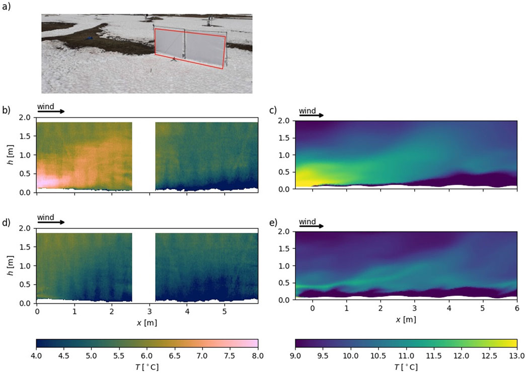
Figure 4. Comparisons of snapshots from measurements using the IR screen setup (Haugeneder et al., 2023) with snapshots from the LES simulations visualizing intermittent advection. The data show along-wind slices through the near-surface boundary layer. The picture in (A) depicts the experimental setup for the IR screen method, and the red frame indicates the excerpt shown in (B, D). (C, E) depict LES data. The wind blows from left to right across the bare ground - snow transition which is at
In the simulation, the layer of cold air adjacent to the snow surface appears to be more clearly separated from the air above. This is especially obvious from the videos in the Supplementary Material. You can see that in the simulation, the wind influences the growth of this layer. However, especially at the leading edge of the snow patch, the depth does not change as much over time as expected from the measurements. This could be explained by vertical wind speeds that are too low and, thus, insufficient vertical mixing. We found from previous simulation runs that the vertical wind speed is an important factor in determining the thickness of the cold air layer in the simulation results. With an underestimated vertical wind speed, there is insufficient vertical mixing to develop a deeper layer of cold air. With a finer grid, we could increase the vertical wind speeds near the surface. However, the fluctuations are still too low as the reader can also see from the comparison in Figure 3C at 1.2 m above the surface.
Just a few seconds after the advection of the warm air plume, the boundary layer near the surface was distinctly colder, as shown in Figures 4D, E. In the measurement, the layer of cold air adjacent to the snow surface was deeper. Air is significantly colder than in Figure 4C, but some slightly warmer plumes as remnants of a previously advected plume detached from the surface, are visible. A deeper layer of decoupled cold air adjacent to the snow surface develops at the leading edge of the snow patch during more quiescent conditions. The cold air even spreads over bare ground because rising buoyant plumes further to the left lead to a local back-flow close to the surface, sucking in cold air from over the snow. The short time difference between the respective two snapshots emphasizes the strong temporal heterogeneity of the near-surface boundary layer apparent in both the simulation results and the measurements.
The offset in absolute temperature between the measurement and the simulation can be explained by the temperature forcing. Using air temperatures measured at 3.7 m above the surface at the AWS (see Figure 1), we do not expect a perfect match. The focus is more on the temporal heterogeneity caused by local surface-driven buoyancy effects. Based on the comparison of time series and spectra between measurement and results, Figure 4 demonstrates that our LES model setup is capable of resolving the measured pattern in the dynamics of the near-surface boundary layer above the transition from bare ground to snow. Furthermore, the above comparison shows the value of visualization using the IR screen setup.
4.2 Buoyancy fluxes and stable internal boundary layer growth
By employing EC sensors in the field, we can gather a temporal sequence of data at specific locations. However, it is difficult or even impossible to interpolate or extrapolate the data to regions without sensors spatially. Especially very close to the surface, within the lowest tens of centimeters, most traditional EC sensors do not yield reliable results. Therefore, the data obtained from the validated LES simulation presented in this study is a powerful tool for investigating spatial properties of the near-surface boundary layer. In the following, we investigate the spatial pattern of median buoyancy flux and the growth of the SIBL adjacent to the snow surface downwind of the transition from bare ground to snow.
We therefore calculate the buoyancy fluxes at every grid point of the along-wind slice taken out of the LES simulation. Figure 5A shows the spatial pattern. For the interpretation, the reader should keep in mind that the simulation tends to underestimate vertical wind speeds and, thus, also buoyancy fluxes. The emphasis is here on spatial patterns without claiming full quantitative accuracy. For a median SIBL depth, we take the median of the buoyancy fluxes time series at every grid point. We define the upper boundary of the SIBL by the sign change of the buoyancy fluxes. Within the SIBL, negative (downward) fluxes prevail. While above the SIBL the stratification in our setting is unstable in accordance with positive (upward) fluxes. Figure 5B depicts the diagnosed SIBL depth as a function of fetch distance over snow,
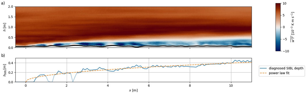
Figure 5. (A) Median buoyancy fluxes in an along-wind cross section through the flow.
We exclude the two drops in the diagnosed SIBL height around
Two different regimes immediately become obvious from Figure 5A. Negative (downward) buoyancy fluxes prevail close to the snow surface. In contrast, the rest of the domain exclusively exhibits positive fluxes. The air heats up over bare ground and is then intermittently advected over the snow surface. Along the trajectory of the plumes, we detect the maximum positive buoyancy fluxes, because warm plumes
The SIBL depth depicted in Figure 5B can be nicely described by the fit reviewed in Brutsaert (1982). At the very leading edge
4.3 Near-surface boundary layer for low and high wind speeds
The results of the LES simulation are well suited to study not only the median flow properties but also the influence of the ambient wind speed on the near-surface boundary layer. In the following, we examine how the near-surface boundary layer changes during periods of low and high wind speeds. We therefore filter the data using the wind speed at
Figure 6 compares vertical profiles for both classes. The temperature profiles in Figures 6A, B show a growing depth of the statically stable layer close to the surface with fetch distance. Furthermore, a dependency of its depth on the wind speed is apparent. Higher wind speeds coincide with shallower statically stable layers. For example, the depth difference at
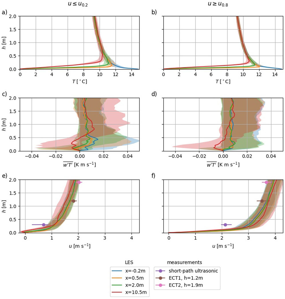
Figure 6. Vertical profiles for two wind speed classes: The left column (a, c, e) contains data with the horizontal wind speed
Layers of different stability also leave their footprints in the profiles of the horizontal wind speed shown in Figures 6E, F. During the quiescent periods the profile at
To further study the heat transfer, especially close to the surface, where reliable measurements are challenging, Figure 7 shows buoyancy fluxes and diagnosed SIBL depths for low and high wind speeds. The setup for each wind speed class is similar to Figure 5. In line with the discussion of the profiles above, we can directly see that the layer of negative fluxes adjacent to the snow surface, the SIBL, is deeper for low wind speeds. The power-law fit yields a SIBL depth at
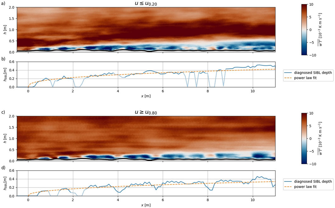
Figure 7. (A) Median buoyancy flux for the
We see from Figure 7 that the buoyancy fluxes within the SIBL are spatially heterogeneous. There are regions with pronounced negative buoyancy fluxes next to regions with positive fluxes. Especially during periods of high wind speeds (Figure 7D), sharp transitions between these regions of fluxes with opposite signs are apparent. This horizontal flux divergence seems to be driven by an interplay of the local wind field with the topography. It points to the fact that the SIBL, and the atmospheric layer adjacent to the snow patch generally, is spatio-temporally highly heterogeneous.
In order to also explore the influence of air temperature on the growth of the SIBL, we conducted further analysis. However, we found that near-surface air temperatures had negligible effects. We provide a figure showing the SIBL growth for low and high air temperatures (similar to Figure 7), along with a brief analysis, in the supplement.
5 Conclusions, limitations, and outlook
In the present study, we set up a centimeter-resolution large eddy simulation to model the near-surface atmospheric flow across an idealized transition from bare ground to snow. We force the inflow-outflow model with high-frequency eddy covariance data recorded during a comprehensive field campaign in patchy snow conditions. Validation with independent high-frequency data shows that the model can reasonably reproduce horizontal wind speed and energy density spectra. However, the model lacks vertical motion and some high-frequency air temperature fluctuations as captured by the measurements. Sensitivity analysis indicates that this disparity may stem from the cell size. Within this highly heterogeneous setting, some energy-containing eddies appear smaller than the chosen horizontal grid spacing of 4 cm. We explain this for the following reasons: (1) artificially smoothed surface, (2) insufficient inflow description and (3) restriction of large-scale motions through the model domain dimensions. As our sensitivity analyses indicate, even state-of-the-art subgrid-scale models cannot adequately parameterize these effects on the centimeter scale. Vertical exchange is a crucial factor determining the structure of the near-surface atmosphere. The lack of representation by our model might lead to an underestimation of the SIBL depths and points to the need for improvements. However, we think that semi-quantitative analyses as presented above still offer valuable insights into the SIBL dynamics. Furthermore, the model adeptly reproduces flow features observed using measurements with a thermal infrared camera pointing at vertically deployed thin synthetic screens. It accurately depicts buoyant plumes of warm air intermittently detaching from the bare ground and being transported over the snow surface. This process is highly dynamic with time scales of only a few seconds. In addition, the simulation results enable us to investigate the growth of a thermal stable internal boundary layer (SIBL) adjacent to the snow surface. We show that the upper boundary of the SIBL can be well described by a power law as suggested by the literature. Moreover, by distinguishing quiescent periods from periods with higher wind speeds, we can show that the wind speed influences the growth of the SIBL. A slightly deeper SIBL can develop with low wind speeds, while higher wind speeds limit its growth. The results also show that the buoyancy fluxes are spatially heterogeneous and driven by terrain roughness even within the lowest layer adjacent to the surface.
Our simulations suggest two further research directions: First, using a finer grid could improve the representation of small-scale turbulence near the surface, especially vertical exchange. This could be achieved by nesting a smaller-domain DNS within the current LES setup to focus on the atmosphere adjacent to the surface. Second, extending the domain with a coarser grid is crucial for developing a physically grounded parameterization of atmospheric processes over highly heterogeneous surfaces. Incorporating actual snow cover distributions as a lower boundary condition helps to quantify the energy exchange between snow and atmosphere on a larger scale spanning tens to hundreds of meters. These scales align with those typically employed in state-of-the-art regional-scale numerical weather models, enabling direct comparisons between the two modeling estimates. The obtained results may be relevant not only for snow hydrological modeling but also for enhancing the performance of atmospheric models.
Data availability statement
The datasets for this study can be found under https://www.doi.org/10.16904/envidat.500. The source code for the analysis presented in this study is accessible under https://github.com/michhau/les_paper_24/tree/main.
Author contributions
MH: Conceptualization, Data curation, Formal Analysis, Investigation, Methodology, Software, Validation, Visualization, Writing–original draft, Writing–review and editing. ML: Conceptualization, Funding acquisition, Methodology, Project administration, Supervision, Writing–review and editing. OH: Investigation, Methodology, Software, Writing–review and editing. MJ: Investigation, Methodology, Software, Writing–review and editing. DR: Investigation, Methodology, Writing–review and editing. RM: Conceptualization, Funding acquisition, Methodology, Project administration, Supervision, Writing–original draft, Writing–review and editing.
Funding
The author(s) declare that financial support was received for the research, authorship, and/or publication of this article. This work is funded by the Swiss National Science Foundation (SNF) project “Snow–atmosphere interactions in mountains: Assessing wind-driven coupling processes and snow-albedo-temperature feedbacks” (nr. 188554). Open access funding by Swiss Federal Institute for Forest, Snow and Landscape Research (WSL).
Acknowledgments
We thank the three anonymous reviewers for their valuable and constructive comments. Furthermore, our gratitude goes to Larissa Schädler for recording UAV orthophotos and assisting during the field campaign. Moreover, we acknowledge OpenAI ChatGPT that we used for language editing of the manuscript.
Conflict of interest
The authors declare that the research was conducted in the absence of any commercial or financial relationships that could be construed as a potential conflict of interest.
The author(s) declared that they were an editorial board member of Frontiers, at the time of submission. This had no impact on the peer review process and the final decision.
Publisher’s note
All claims expressed in this article are solely those of the authors and do not necessarily represent those of their affiliated organizations, or those of the publisher, the editors and the reviewers. Any product that may be evaluated in this article, or claim that may be made by its manufacturer, is not guaranteed or endorsed by the publisher.
Supplementary material
The Supplementary Material for this article can be found online at: https://www.frontiersin.org/articles/10.3389/feart.2024.1415327/full#supplementary-material
References
Balogh, M., Parente, A., and Benocci, C. (2012). Rans simulation of abl flow over complex terrains applying an enhanced k-ε model and wall function formulation: implementation and comparison for fluent and openfoam. J. Wind Eng. Industrial Aerodynamics 104-106, 360–368. doi:10.1016/j.jweia.2012.02.023
Bavay, M., Lehning, M., Jonas, T., and Löwe, H. (2009). Simulations of future snow cover and discharge in alpine headwater catchments. Hydrol. Process. 23, 95–108. doi:10.1002/hyp.7195
Bradley, E. F. (1968). A micrometeorological study of velocity profiles and surface drag in the region modified by a change in surface roughness. Q. J. R. Meteorological Soc. 94, 361–379. doi:10.1002/qj.49709440111
Brauchli, T., Trujillo, E., Huwald, H., and Lehning, M. (2017). Influence of slope-scale snowmelt on catchment response simulated with the alpine3d model. Water Resour. Res. 53, 10723–10739. doi:10.1002/2017WR021278
Brutsaert, W. (1982). Evaporation into the atmosphere. Springer Netherlands. doi:10.1007/978-94-017-1497-6
Carletti, F., Michel, A., Casale, F., Burri, A., Bocchiola, D., Bavay, M., et al. (2022). A comparison of hydrological models with different level of complexity in alpine regions in the context of climate change. Hydrology Earth Syst. Sci. 26, 3447–3475. doi:10.5194/hess-26-3447-2022
Deardorff, J. W. (1974). Three-dimensional numerical study of the height and mean structure of a heated planetary boundary layer. Boundary-Layer Meteorol. 7, 81–106. doi:10.1007/BF00224974
Elliott, W. P. (1958). The growth of the atmospheric internal boundary layer. Eos, Trans. Am. Geophys. Union 39, 1048–1054. doi:10.1029/TR039i006p01048
Farina, S., and Zardi, D. (2023). Understanding thermally driven slope winds: recent advances and open questions. Boundary-Layer Meteorol. 189, 5–52. doi:10.1007/s10546-023-00821-1
Föhn, P. M. B., and Meister, R. (1983). Distribution of snow drifts on ridge slopes: measurements and theoretical approximations. Ann. Glaciol. 4, 52–57. doi:10.3189/S0260305500005231
Garratt, J. R. (1990). The internal boundary layer - a review. Boundary-Layer Meteorol. 50, 171–203. doi:10.1007/BF00120524
Gerber, F., Mott, R., and Lehning, M. (2019). The importance of near-surface winter precipitation processes in complex alpine terrain. J. Hydrometeorol. 20, 177–196. doi:10.1175/JHM-D-18-0055.1
Germano, M., Piomelli, U., Moin, P., and Cabot, W. H. (1991). A dynamic subgrid-scale eddy viscosity model. Phys. Fluids A Fluid Dyn. 3, 1760–1765. doi:10.1063/1.857955
Granger, R. J., Essery, R., and Pomeroy, J. W. (2006). Boundary-layer growth over snow and soil patches: field observations. Hydrol. Process. 20, 943–951. doi:10.1002/hyp.6123
Groffman, P. M., Driscoll, C. T., Fahey, T. J., Hardy, J. P., Fitzhugh, R. D., and Tierney, G. L. (2001). Colder soils in a warmer world: a snow manipulation study in a northern hardwood forest ecosystem. Biogeochemistry 56, 135–150. doi:10.1023/A:1013039830323
Grudzielanek, A. M., and Cermak, J. (2015). Capturing cold-air flow using thermal imaging. Boundary-Layer Meteorol. 157, 321–332. doi:10.1007/s10546-015-0042-8
Hames, O., Jafari, M., Wagner, D. N., Raphael, I., Clemens-Sewall, D., Polashenski, C., et al. (2022). Modeling the small-scale deposition of snow onto structured arctic sea ice during a mosaic storm using snowbedfoam 1.0. Geosci. Model Dev. 15, 6429–6449. doi:10.5194/gmd-15-6429-2022
Harder, P., Pomeroy, J. W., and Helgason, W. (2017). Local-scale advection of sensible and latent heat during snowmelt. Geophys. Res. Lett. 44, 9769–9777. doi:10.1002/2017GL074394
Haugeneder, M., Lehning, M., Reynolds, D., Jonas, T., and Mott, R. (2023). A novel method to quantify near-surface boundary-layer dynamics at ultra-high spatio-temporal resolution. Boundary-Layer Meteorol. 186, 177–197. doi:10.1007/s10546-022-00752-3
Haugeneder, M., Lehning, M., Stiperski, I., Reynolds, D., and Mott, R. (2024). Turbulence in the strongly heterogeneous near-surface boundary layer over patchy snow. Boundary-Layer Meteorol. 190, 7. doi:10.1007/s10546-023-00856-4
Högström, U. (1996). Review of some basic characteristics of the atmospheric surface layer. Boundary-Layer Meteorol. 78, 215–246. doi:10.1007/BF00120937
Huang, J., and Bou-Zeid, E. (2013). Turbulence and vertical fluxes in the stable atmospheric boundary layer. part i: a large-eddy simulation study. J. Atmos. Sci. 70, 1513–1527. doi:10.1175/JAS-D-12-0167.1
Jafari, M., Sharma, V., and Lehning, M. (2022). Convection of water vapour in snowpacks. J. Fluid Mech. 934, A38. doi:10.1017/jfm.2021.1146
Johnson, R. H., Young, G. S., Toth, J. J., and Zehr, R. M. (1984). Mesoscale weather effects of variable snow cover over northeast Colorado. Mon. Weather Rev. 112, 1141–1152. doi:10.1175/1520-0493(1984)112<1141:mweovs>2.0.co;2
Kljun, N., Calanca, P., Rotach, M. W., and Schmid, H. P. (2015). A simple two-dimensional parameterisation for flux footprint prediction (ffp). Geosci. Model Dev. 8, 3695–3713. doi:10.5194/gmd-8-3695-2015
Kolmogorov, A. N. (1941). The local structure of turbulence in incompressible viscous fluid for very large Reynolds numbers. Dokl. Akad. Nauk. SSSR 30, 301–304.
Lehning, M., Löwe, H., Ryser, M., and Raderschall, N. (2008). Inhomogeneous precipitation distribution and snow transport in steep terrain. Water Resour. Res. 44. doi:10.1029/2007WR006545
Lehning, M., Völksch, I., Gustafsson, D., Nguyen, T. A., Stähli, M., and Zappa, M. (2006). Alpine3d: a detailed model of mountain surface processes and its application to snow hydrology. Hydrol. Process. 20, 2111–2128. doi:10.1002/hyp.6204
Leslie, D. C., and Quarini, G. L. (1979). The application of turbulence theory to the formulation of subgrid modelling procedures. J. Fluid Mech. 91, 65. doi:10.1017/S0022112079000045
Letcher, T. W., and Minder, J. R. (2017). The simulated response of diurnal mountain winds to regionally enhanced warming caused by the snow albedo feedback. J. Atmos. Sci. 74, 49–67. doi:10.1175/JAS-D-16-0158.1
Li, D., Lettenmaier, D. P., Margulis, S. A., and Andreadis, K. (2019). The role of rain-on-snow in flooding over the conterminous United States. Water Resour. Res. 55, 8492–8513. doi:10.1029/2019WR024950
Lund, T. (2003). The use of explicit filters in large eddy simulation. Comput. & Math. Appl. 46, 603–616. doi:10.1016/S0898-1221(03)90019-8
Magnusson, J., Nævdal, G., Matt, F., Burkhart, J. F., and Winstral, A. (2020). Improving hydropower inflow forecasts by assimilating snow data. Hydrology Res. 51, 226–237. doi:10.2166/nh.2020.025
Melo, D. B., Sigmund, A., and Lehning, M. (2024). Understanding snow saltation parameterizations: lessons from theory, experiments and numerical simulations. Cryosphere 18, 1287–1313. doi:10.5194/tc-18-1287-2024
Ménard, C. B., Essery, R., and Pomeroy, J. (2014). Modelled sensitivity of the snow regime to topography, shrub fraction and shrub height. Hydrology Earth Syst. Sci. 18, 2375–2392. doi:10.5194/hess-18-2375-2014
Meneveau, C., Lund, T. S., and Cabot, W. H. (1996). A Lagrangian dynamic subgrid-scale model of turbulence. J. Fluid Mech. 319, 353. doi:10.1017/S0022112096007379
Mott, R., Daniels, M., and Lehning, M. (2015). Atmospheric flow development and associated changes in turbulent sensible heat flux over a patchy mountain snow cover. J. Hydrometeorol. 16, 1315–1340. doi:10.1175/JHM-D-14-0036.1
Mott, R., Egli, L., Grünewald, T., Dawes, N., Manes, C., Bavay, M., et al. (2011). Micrometeorological processes driving snow ablation in an alpine catchment. Cryosphere 5, 1083–1098. doi:10.5194/tc-5-1083-2011
Mott, R., Gromke, C., Grünewald, T., and Lehning, M. (2013). Relative importance of advective heat transport and boundary layer decoupling in the melt dynamics of a patchy snow cover. Adv. Water Resour. 55, 88–97. doi:10.1016/j.advwatres.2012.03.001
Mott, R., Schlögl, S., Dirks, L., and Lehning, M. (2017). Impact of extreme land surface heterogeneity on micrometeorology over spring snow cover. J. Hydrometeorol. 18, 2705–2722. doi:10.1175/JHM-D-17-0074.1
Mott, R., Winstral, A., Cluzet, B., Helbig, N., Magnusson, J., Mazzotti, G., et al. (2023). Operational snow-hydrological modeling for Switzerland. Front. Earth Sci. 11. doi:10.3389/feart.2023.1228158
Moukalled, F., Mangani, L., and Darwish, M. (2016). The finite volume method in computational fluid dynamics, 113. Springer International Publishing. doi:10.1007/978-3-319-16874-6
OpenFoam API Guide (2024). buoyantboussinesqpimplefoam.c file reference. Available at: https://www.openfoam.com/documentation/guides/latest/api/buoyantBoussinesqPimpleFoam_8C.html (Accessed April 3, 2024).
Poletto, R., Craft, T., and Revell, A. (2013). A new divergence free synthetic eddy method for the reproduction of inlet flow conditions for les. Flow, Turbul. Combust. 91, 519–539. doi:10.1007/s10494-013-9488-2
Pomeroy, J., and Gray, D. (1995). Snowcover accumulation, relocation and management NHRI science report No. Natl. Hydrology Res. Inst.
Quéno, L., Mott, R., Morin, P., Cluzet, B., Mazzotti, G., and Jonas, T. (2023). Snow redistribution in an intermediate-complexity snow hydrology modelling framework. EGUsphere 2023, 1–32. doi:10.5194/egusphere-2023-2071
Reynolds, D., Gutmann, E., Kruyt, B., Haugeneder, M., Jonas, T., Gerber, F., et al. (2023). The high-resolution intermediate complexity atmospheric research (hicar v1.1) model enables fast dynamic downscaling to the hectometer scale. Geosci. Model Dev. 16, 5049–5068. doi:10.5194/gmd-16-5049-2023
Reynolds, D., Quéno, L., Lehning, M., Jafari, M., Berg, J., Jonas, T., et al. (2024). Seasonal snow-atmosphere modeling: let’s do it. EGUsphere 2024, 1–28. doi:10.5194/egusphere-2024-489
Richardson, H., Basu, S., and Holtslag, A. A. M. (2013). Improving stable boundary-layer height estimation using a stability-dependent critical bulk richardson number. Boundary-Layer Meteorol. 148, 93–109. doi:10.1007/s10546-013-9812-3
Rixen, C., Høye, T. T., Macek, P., Aerts, R., Alatalo, J. M., Anderson, J. T., et al. (2022). Winters are changing: snow effects on arctic and alpine tundra ecosystems. Arct. Sci. 8, 572–608. doi:10.1139/as-2020-0058
Schlögl, S., Lehning, M., Fierz, C., and Mott, R. (2018a). Representation of horizontal transport processes in snowmelt modeling by applying a footprint approach. Front. Earth Sci. 6. doi:10.3389/feart.2018.00120
Schlögl, S., Lehning, M., and Mott, R. (2018b). How are turbulent sensible heat fluxes and snow melt rates affected by a changing snow cover fraction? Front. Earth Sci. 6. doi:10.3389/feart.2018.00154
Schotanus, P., Nieuwstadt, F., and Bruin, H. D. (1983). Temperature measurement with a sonic anemometer and its application to heat and moisture fluxes. Boundary-Layer Meteorol. 26, 81–93. doi:10.1007/BF00164332
Sigmund, A., Dujardin, J., Comola, F., Sharma, V., Huwald, H., Melo, D. B., et al. (2022). Evidence of strong flux underestimation by bulk parametrizations during drifting and blowing snow. Boundary-Layer Meteorol. 182, 119–146. doi:10.1007/s10546-021-00653-x
Siirila-Woodburn, E. R., Rhoades, A. M., Hatchett, B. J., Huning, L. S., Szinai, J., Tague, C., et al. (2021). A low-to-no snow future and its impacts on water resources in the western United States. Nat. Rev. Earth & Environ. 2, 800–819. doi:10.1038/s43017-021-00219-y
Smagorinski, J. (1963). General circulation experiments with the primitive equations. Mon. Weather Rev. 91, 99–164. doi:10.1175/1520-0493(1963)091<0099:gcewtp>2.3.co;2
Smith, C. M., and Porté-Agel, F. (2014). An intercomparison of subgrid models for large-eddy simulation of katabatic flows. Q. J. R. Meteorological Soc. 140, 1294–1303. doi:10.1002/qj.2212
Stiperski, I., and Rotach, M. W. (2016). On the measurement of turbulence over complex mountainous terrain. Boundary-Layer Meteorol. 159, 97–121. doi:10.1007/s10546-015-0103-z
Stoll, R., Gibbs, J. A., Salesky, S. T., Anderson, W., and Calaf, M. (2020). Large-eddy simulation of the atmospheric boundary layer. Boundary-Layer Meteorol. 177, 541–581. doi:10.1007/s10546-020-00556-3
Stucchi, L., Bombelli, G., Bianchi, A., and Bocchiola, D. (2019). Hydropower from the alpine cryosphere in the era of climate change: the case of the sabbione storage plant in Italy. Water 11, 1599. doi:10.3390/w11081599
Stull, R. B. (1988). An introduction to boundary layer meteorology. Springer Netherlands. doi:10.1007/978-94-009-3027-8
Sturm, M., Goldstein, M. A., and Parr, C. (2017). Water and life from snow: a trillion dollar science question. Water Resour. Res. 53, 3534–3544. doi:10.1002/2017WR020840
Sui, J., and Koehler, G. (2001). Rain-on-snow induced flood events in southern Germany. J. Hydrology 252, 205–220. doi:10.1016/S0022-1694(01)00460-7
Takahara, H., and Higuchi, K. (1985). Thermal modification of air moving over melting snow surfaces. Ann. Glaciol. 6, 235–237. doi:10.3189/1985AoG6-1-235-237
Urfer-Henneberger, C. (1970). Neuere beobachtungen über die entwicklung des schönwetterwindsystems in einem v-förmigen alpental (dischmatal bei davos). Arch. für Meteorol. Geophys. Bioklimatol. Ser. B 18, 21–42. doi:10.1007/BF02245866
van der Valk, L. D., Teuling, A. J., Girod, L., Pirk, N., Stoffer, R., and van Heerwaarden, C. C. (2022). Understanding wind-driven melt of patchy snow cover. Cryosphere 16, 4319–4341. doi:10.5194/tc-16-4319-2022
Weisman, R. N. (1977). Snowmelt: a two-dimensional turbulent diffusion model. Water Resour. Res. 13, 337–342. doi:10.1029/WR013i002p00337
Weller, H. G., Tabor, G., Jasak, H., and Fureby, C. (1998). A tensorial approach to computational continuum mechanics using object-oriented techniques. Comput. Phys. 12, 620–631. doi:10.1063/1.168744
Wever, N., Comola, F., Bavay, M., and Lehning, M. (2017). Simulating the influence of snow surface processes on soil moisture dynamics and streamflow generation in an alpine catchment. Hydrology Earth Syst. Sci. 21, 4053–4071. doi:10.5194/hess-21-4053-2017
Wheeler, J. A., Cortés, A. J., Sedlacek, J., Karrenberg, S., van Kleunen, M., Wipf, S., et al. (2016). The snow and the willows: earlier spring snowmelt reduces performance in the low-lying alpine shrub Salix herbacea. J. Ecol. 104, 1041–1050. doi:10.1111/1365-2745.12579
Wipf, S., and Rixen, C. (2010). A review of snow manipulation experiments in arctic and alpine tundra ecosystems. Polar Res. 29, 95–109. doi:10.1111/j.1751-8369.2010.00153.x
Würzer, S., Jonas, T., Wever, N., and Lehning, M. (2016). Influence of initial snowpack properties on runoff formation during rain-on-snow events. J. Hydrometeorol. 17, 1801–1815. doi:10.1175/JHM-D-15-0181.1
Zahn, E., and Bou-Zeid, E. (2024). Setting up a large-eddy simulation to focus on the atmospheric surface layer. Boundary-Layer Meteorol. 190, 12. doi:10.1007/s10546-023-00841-x
Keywords: large eddy simulation, near-surface boundary layer, turbulence, patchy snow, stable internal boundary layer, buoyancy flux
Citation: Haugeneder M, Lehning M, Hames O, Jafari M, Reynolds D and Mott R (2024) Large eddy simulation of near-surface boundary layer dynamics over patchy snow. Front. Earth Sci. 12:1415327. doi: 10.3389/feart.2024.1415327
Received: 10 April 2024; Accepted: 01 October 2024;
Published: 29 October 2024.
Edited by:
Satoru Yamaguchi, National Research Institute for Earth Science and Disaster Resilience (NIED), JapanReviewed by:
Bangjun Cao, Chengdu University of Information Technology, ChinaYanzhao Zhou, Hebei Normal University, China
Kezhen Chong, Pacific Northwest National Laboratory (DOE), United States
Copyright © 2024 Haugeneder, Lehning, Hames, Jafari, Reynolds and Mott. This is an open-access article distributed under the terms of the Creative Commons Attribution License (CC BY). The use, distribution or reproduction in other forums is permitted, provided the original author(s) and the copyright owner(s) are credited and that the original publication in this journal is cited, in accordance with accepted academic practice. No use, distribution or reproduction is permitted which does not comply with these terms.
*Correspondence: Michael Haugeneder, bWljaGFlbC5oYXVnZW5lZGVyQHNsZi5jaA==