 Sebastian Pessenlehner
 Philipp Gmeiner1,2
 Marcel Liedermann
- 1Institute of Hydraulic Engineering and River Research, Department of Water, Atmosphere, and Environment, University of Natural Resources and Life Sciences, Vienna, Austria
- 2Christian Doppler Laboratory for Sediment Research and Management, Vienna, Austria
Plastic pollution in aquatic environments is a growing concern, with rivers recognized as major pathways. However, rivers themselves are also subject to pollution. Hence, understanding riverine plastic transport dynamics is essential for mitigating environmental impacts. Although plastic-related research focus has shifted from marine environments towards rivers, challenges remain in standardizing methods for monitoring and integrating spatio-temporal variabilities of riverine plastic occurrence into flux determination. This study addresses these challenges by adopting established methods from sediment research. Utilizing data from a net-based cross-sectional multi-point approach, it examines spatio-temporal and discharge-dependent variations. It comprehensively analyzes the complex dynamics of plastic transport in the Danube River, contrasting an impounded section near Aschach, Austria, with a free-flowing reach near Hainburg, Austria. The paper emphasizes the significance of applying these methodologies for accurate flux determination and underscores the risks of neglecting them. By incorporating average microplastic particle weights, we aim to overcome limitations in prior methodologies that solely emphasize qualitative aspects or rely on item numbers. Spatial distribution analysis revealed a pronounced stratification at low flow and a more variable distribution in the free-flowing section, attributed to higher turbulence. As discharge increased, vertical mixing occurred, along with distinct lateral patterns displaying increased concentrations toward the riverbanks. Encountering plastic particles throughout the river profile underscores their properties of both suspended and floating matter, emphasizing the importance of hydro-morphology and multi-point cross-sectional measurement approaches. Microplastic loads were calculated to be <6.9 t a−1 in Aschach and <17.1 t a−1 in Hainburg, compared to total plastic loads of <14.3 t a−1 in Aschach and <41.6 t a−1 in Hainburg. Consequently, plastic loads were doubled to tripled within the Austrian section of the Danube River. The study contributes valuable insights into the complex nature of plastic transport in river systems, emphasizing comprehensive spatial, temporal and discharge-dependent assessments for characterizing and managing plastic pollution. It suggests that rivers can function as sources, pathways and sinks of plastic pollution, contingent upon hydro-morphological conditions. This underscores the need for longitudinal, basin-wide assessments to accurately understand plastic transport dynamics.
1 Introduction
Rivers are increasingly recognized as substantial contributors of plastic debris to marine environments, thereby posing significant environmental concerns due to the longevity of these polymers and their potential long-term impacts on biota (Lebreton et al., 2017; Liedermann et al., 2018; van Emmerik and Schwarz, 2020; Meijer et al., 2021; Blondel and Buschman, 2022; Range et al., 2023; van Emmerik et al., 2023). Besides being considered as primary transport paths from land-based sources to the sea, it is important to note that rivers themselves are also subject to pollution from plastic debris (Meijer et al., 2021; Lofty et al., 2023; Range et al., 2023) and may rather act as (temporal) sinks and reservoirs, particularly in tidal zones (van Emmerik et al., 2022b; van Emmerik et al., 2023). Entry paths reach from direct disposal from e.g., littering or recycled wastewater to airborne dispersal up to flood induced mobilization (Allen et al., 2019; Woodward et al., 2021; Lofty et al., 2023). However, their role in linking sources and sinks is insufficiently understood. Consequently, there has been a noticeable shift in research focus from marine environments towards the monitoring and comprehension of riverine plastic transport, as evidenced by numerous case studies, review papers, and meta-analyses (Lofty et al., 2023; Range et al., 2023).
The transport processes of riverine plastic debris are inherently complex due to their diverse physical properties, including (i) type, (ii) size, (iii) shape and (iv) density (Range et al., 2023). All these characteristics significantly influence the spatio-temporal appearance in flowing waters. Comprising a wide range of polymer types, plasticserves as a source of hazardous compounds by leaching of e.g., persistent pollutants and toxic additives. Especially fragmented and small particleshave the capability to adsorb and accumulate contaminants such as antibiotics, and heavy metals, thereby acting as vectors of these pollutants in the water cycle (Bakir et al., 2014; Hohenblum et al., 2015; Hermabessiere et al., 2017; Zhang et al., 2020; Range et al., 2023). Due to their diverse origins and the degradation processes of larger plastic waste, microplastic particles–commonly defined as particles smaller than 5 mm (Cole et al., 2011; Anderson et al., 2016)—appear in various shapes such as fragments, pellets, fibres, and films, either as primary or secondary microplastics (Hartmann et al., 2019). The small size of microplastic particles furthermore increases their bioavailability to organisms, with limited selectivity in capturing any particles of appropriate size (Wright et al., 2013). Another significant parameter influencing the spatio-temporal transport processes is density, which, in conjunction with size, shape, aggregation (clustering of particles) and the growth of biofilms, influences the buoyancy of microplastic particles, resulting in them being either floating, neutral, or sinking (Cole et al., 2011; Anderson et al., 2016; Waldschlager and Schuttrumpf, 2019).
As monitoring plastic transport in rivers gained importance on a global scale, riverine transport of microplastic is increasingly studied as reviewed by Range et al. (2023) or Lofty et al. (2023). However, discussions within the scientific community regarding suitable methods for field sampling, analysis and quantification to address and understand riverine plastic transport have emerged (Skalska et al., 2020; Lofty et al., 2023; Range et al., 2023). Related to field sampling it is crucial to differentiate between methods appropriate for microplastics and those for macroplastics. For larger macroplastics, besides net sampling (Blondel and Buschman, 2022), also GPS-tracking (Tramoy et al., 2020), visual approaches via counting from bridges (González-Fernández and Hanke, 2017; van Emmerik et al., 2018), utilization of automated camera systems (van Lieshout et al., 2020) and spaceborne UAVs (Geraeds et al., 2019), or interpretation of ADCP backscatter signals (Broere et al., 2021; Boon et al., 2023) are commonly employed. On the other hand, for microplastics, multi-depth net-based sampling devices with a typical mesh size around 300 μm (Liedermann et al., 2018; Lenaker et al., 2019; Stock et al., 2019), as well as pump sampling systems (Prata et al., 2019; Stock et al., 2019; Bordos et al., 2021) utilizing fractionated pressure filter cascades (typically with cascades of 100, 20, and 5 μm), are commonly employed as direct sampling methods. Advantages and disadvantages related to application, sampling volume, sample analysis etc. between those methods are described in literature (e.g., in Stock et al., 2019; Range et al., 2023; Lofty et al., 2023). Additionally, indirect methods such as model approaches and algorithms to link measured plastic concentrations to satellite images or suspended sediment concentrations have been explored in several studies (Mohsen et al., 2023; Range et al., 2023). Similar to the field of sediment monitoring, these remote sensing approaches attempt to find cost-effective solutions for comprehensive monitoring of plastics in rivers, while still depending on data from direct sampling.
However, despite the limited number of studies focusing on quantitative microplastic transport (e.g., Hohenblum et al., 2015; Liedermann et al., 2018; Eo et al., 2019; Mani and Burkhardt-Holm, 2020; Haberstroh et al., 2021; Treilles et al., 2022), many published studies focus on qualitative aspects, lacking in-depth quantification by disregarding spatio-temporal aspects, or only rely on item numbers instead of mass transport (Skalska et al., 2020; Range et al., 2023). This is primarily because sound spatio-temporal measurements are labor-intensive, and determining masses is more complex than counting particles. Nonetheless, neglecting these documented spatio-temporal variabilities and applying inadequate transport calculation methods can lead to significant over- or underestimation of plastic loads (Range et al., 2023). Furthermore, using item number as a unit for quantitative assessment of fluxes and annual loads is insufficient, especially considering fragmentation processes and using numbers as a basis for global-scale policies (Skalska et al., 2020; Range et al., 2023). Attempts to establish correlations between item numbers and masses have been made using sophisticated methods considering the density, shapes, and sizes of the particles encountered (Kooi and Koelmans, 2019; Koelmans et al., 2020; Range et al., 2023). Yet reliable data sets based on mass determination are essential for meaningful correlations.
As presented in this study, alongside a suitable monitoring method, further key requirements are suitable calculation methods for plastic transport and annual loads. According to Liedermann et al. (2018) and Range et al. (2023), the quantification of microplastic transport should follow the established quantification methods of suspended sediment research, as also here the spatial and temporal integration are the decisive factors. To demonstrate the significance of suitable measurement and quantification approaches, the presented study builds upon data from a well-established monitoring approach introduced by Liedermann et al. (2018), which utilizes a net-based multi-depth plastic sampling device. In the past decade, this measurement system has undergone adjustments, optimizations, and applications across a wide range of boundary conditions. Numerous multi-point measurement campaigns have been conducted along the Danube River in Austria, Hungary, Serbia, and Romania as part of various research studies. This study, however, uses a robust database covering a wide discharge spectrum along the Austrian Danube River. Thus, it enables to emphasize the importance of (i) spatio-temporal isokinetic sampling, (ii) systematic data processing, (iii) suitable calculation methods for spatial integration of plastic transport, (iv) the establishment of appropriate rating curves used for item- and mass-based transport calculations, and (v) reveals insights into the transport processes of plastics in a large river.
2 Study sites
The data set utilized in this study was gathered between September 2014 and February 2015 through net-based multipoint plastic measurements covering various hydrological conditions from low flow to flood discharges. These measurements were conducted in two distinct cross-sections at the Austrian Danube River, situated near Aschach (River-km 2159.96; 48°21′45.3″N, 14°01′32.7″E) and Hainburg (River-km 1886.24; 48°08′47.5″N, 16°54′29.4″E) as depicted in Figure 1. The locations were chosen due to their proximity to the entrance and exit of the Danube River in Austria, as well as for logistical convenience, given the presence of road bridges essential for sampling with the multi-depth net device especially at high discharges.

Figure 1. Overview of the project area with the two measurement sites near Aschach and Hainburg at the Austrian Danube River (Data sources: National borders–Eurostat data; Cities, Rivers, Danube River Basin District–ICPDR DanubeGIS; Rivers–eHAO Hydrologischer Atlas Österreich; Background: Esri, USGS, NOAA, World Terrain Base), including a picture of the used multi-depth net-based sampling devices (adapted after Liedermann et al., 2018).
Both sites, situated within the Upper Danube sub-basin, feature a relatively steep slope of around 0.0004 and are characterized by gravel sediments. However, regarding the morphological and hydraulic boundary conditions, the chosen locations differ significantly. At Aschach, the upstream monitoring site, the Danube is classified as a heavily modified waterbody according to International Commission for the Protection on the Danube River (ICPDR, 2015). The straight section is surrounded by settlements and the riverbanks are secured by riprap embankments. Lying within a chain of hydropower plants, the hydraulic characteristics of the river are primarily dominated by the impoundment of the downstream hydropower plant Ottensheim-Wilhering. At the gauge Aschach-Agentie (river-km 2159.73) the regulated low flow discharge (referred to as RNQ, exceeded 94% of the time) equals 755 m3 s−1, the annual mean discharge (MQ) is 1,450 m3 s−1, the highest navigable discharge (1% exceedance duration) is 3,530 m3 s−1 and the 1-year flood event (HQ1) yields 4,000 m3 s−1 according to the Austrian waterways authority via donau (via donau, 2012). The catchment size at the Aschach study site amounts to 78,190 km2. The cross-section features a width of 230 m and a depth of around 8.0 m during mean flow conditions with only minor water level changes, due to the impoundment, and average flow velocities of only 0.5–1.5 m s−1.
Near Hainburg, on the other hand, the Danube River lies within the Donau-Auen National Park and represents one of two remaining free-flowing sections of the Austrian Danube River. The reach is characterised by a 30° right river bend, with partly natural and dynamic riverbanks. Characteristic discharge values at the gauge Hainburg (river-km 1883.96) are 980 m3 s−1 (RNQ), 1,930 m3 s−1 (MQ), 5,130 m3 s−1 (highest navigable and bankfull discharge) and 5,300 m3 s−1 (HQ1) (via donau, 2012). Within low flow to bankfull discharge, the river width ranges between 330 and 350 m, while water depths range from 2.5 to 7.0 m in the main channel of the monitored cross-section. Flow velocities in the main channel vary between 1.5 up to 3.0 m s−1, with a shallower and calmer area on the left bank due to a groyne field. The catchment size of 104,727 km2 equals an areal increase of ∼33% compared to the upstream measurement site, with a similar increase in mean water discharge. On its course from Aschach to Hainburg, the Danube passes several cities (e.g., Linz, Vienna), eight hydropower plants and drains several large tributaries, especially on the orographic right (e.g., Traun, Enns).
3 Materials and methods
3.1 Sampling methodology and sample analysis
3.1.1 Cross-sectional multi-point net measurements
The net-based multi-depth plastic sampling device developed by Liedermann et al. (2018) is designed for robust performance in medium to large rivers, including conditions of flood discharge (see Figure 1). It measures the vertical variability of plastic concentrations by deploying a set of three nets–single or double net frames—at adjustable depths (surface, centre, near-bed) to capture turbulence- and plastic property-induced variations in the water column. To address horizontal variability, the device is lowered at multiple verticals within the sampled cross-section via crane, either from a road bridge or a vessel. The device features 60 by 60 cm inlet openings with mesh sizes of 500 and 250 μm for double net frames, respectively. The filtered water volume is monitored using mechanical impellers mounted at the centre of each net frame. Sampling durations typically last around 30 min, depending on discharge conditions and possible net clogging due to turbidity, the duration was reduced to 5 min for some measurements. Collected samples are accumulated in containers at the net ends, facilitating easy removal and analysis after cleaning the nets with a high-pressure cleaner. Additionally, measurements of flow velocity (e.g., using an ADCP Acoustic Doppler Current Profiler device) throughout the sampled cross-section were made to account for the hydraulic parameters and discharge data.
3.1.2 Sample analysis
A comprehensive and advanced laboratory analysis of plastic samples forms the foundation for subsequent item-, mass-, and type-based evaluations. The process of laboratory preparation process, which is not the main focus of this study is described in Hohenblum et al. (2015) and Liedermann et al. (2018) and involved several steps including sieving, H2O2 treatment to reduce organic matter, drying, visual sorting, weighing, counting and particle type identification. In addition to visual methods, infrared spectroscopy using ATR (Attenuated Total Reflection) and FTIR (Fourier Transform Infrared Spectroscopy) were employed for detecting plastic types, particularly for small particles where visual detection of item numbers is challenging.
Masses and item numbers of each sample were quantified using fractions <5 mm and >5 mm. The size fraction comprising only particles smaller than 5 mm is consequently referred to as microplastic (see Cole et al., 2011; Anderson et al., 2016), while the size fraction also including particles larger than 5 mm is referred to as total plastic. For mass determination, a laboratory balance (ACCULAB, ALC 210.4, Sartorius Group) with an accuracy of ≤±0.1 mg was used to weigh the composite sample of each sampling point and size class. Large macroplastics such as PET bottles or large fragments, however, tended to occur very randomly and seldomly during the measurements. Addressing them properly would require extended measurement times, increased inlet openings, or other monitoring methodologies. Therefore, we excluded these items from the total plastic mass in the analysis.
3.1.2.1 Correlation of particle number and mass
Within this study, attempts were furthermore made to correlate particle numbers and masses for microplastic particles between >500/250 μm and <5 mm. While other authors (Kooi and Koelmans, 2019; Koelmans et al., 2020; Range et al., 2023) suggest complex and labor-intensive procedures based on size, type, shape, and density, we simply sought to correlate the number of counted items and their mass within this size range. Therefore, we simply divided the weight of the composite sample in each sampling point and size class by the item number. The emphasis here was primarily on identifying differences in average particle weight related to measurement depth, discharge, and site.
3.2 Quantification of plastic transport
In sediment research, quantifying solid transport requires considering spatial, temporal, and discharge-dependent variabilities. This typically involves an integrated combination of direct cross-sectional measurements to account for the spatial variability and either indirect sensor-based measurements or establishing rating curves linking water discharge and solid transport to temporal variability (e.g., Walling, 1977; Wass and Leeks, 1999; Asselman, 2000; Horowitz, 2003; Haimann et al., 2014). However, for plastic transport, continuous high-resolution sensors for plastic concentrations are not yet available. Consequently, Liedermann et al. (2018) proposed adopting the methodology of multi-point sampling commonly employed in suspended sediment research, as described in Edwards and Glysson (1999), ISO 4363 (2002) or BMLFUW (2017). In this study, we introduce an adapted methodology and apply it to plastic transport data. This methodology emphasizes the importance of conducting measurements over longer periods, covering the entire discharge spectrum from low flow to flood discharge through multi-point sampling to derive cross-sectional average concentrations and establish rating curves for flux determination. This approach is equally suitable for both masses and item numbers, which we demonstrate in terms of masses below.
3.2.1 Spatial distribution of plastics
To incorporate the spatial distribution of plastics during quantification, in a first step (Equation 1): the plastic concentration
When using double net frames, as performed within this study, it is recommended to first calculate the average plastic concentration for each measured height, to get one concentration value per height and then proceed with the calculation as outlined below.
Besides assessing plastic concentration variability between multiple points within the cross-section (Figure 2A), it is crucial to include the vertical flow velocity distribution during spatial integration (Figure 2B). Consequently, the plastic transport rate
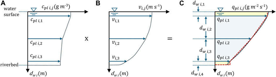
Figure 2. Methodology for calculation of depth-average plastic transport rates
Subsequently, the plastic transport in the cross-section is calculated by spatially integrating the plastic transport rates of each point over the water depth and the width of the measured profile. First the depth-average plastic transport rate
where
The cross-sectional plastic transport
where

Figure 3. Methodology for calculation of cross-sectional plastic transport
The mean discharge-weighted cross-sectional plastic concentration
3.2.1.1 Evaluation of potential errors due to different monitoring strategies
Given the insufficient attention to spatio-temporal aspects in many published studies, a substantial risk of significant over- or underestimation of transport exists (Range et al., 2023). Therefore, this study aims to evaluate potential errors in transport determination, specifically referring to studies that either exclusively consider near-surface (e.g., Dris et al., 2015) or near-bank sampling (e.g., Lechner et al., 2014). While the spatial integration method to calculate the cross-sectional plastic transport remained the same, we varied the input values for plastic concentration:
• mean discharge-weighted cross-sectional plastic concentration: addressing the multi-point cross-sectional sampling method proposed within this study
• near-surface plastic concentration: addressing near-surface cross-sectional sampling methods by including only the average near-surface concentration of each vertical
• near-bank surface sampling: addressing near-bank surface sampling methods by including only the near-bank surface concentration on the right riverbank
3.2.2 Temporal and discharge dependent distribution of microplastics
3.2.2.1 Rating curves and load calculation
An accurate load calculation requires considering the temporal and discharge dependent abundances of plastics. Therefore, rating curves are developed to establish relationships between water discharge and plastic transport, as hydrology is known to play a crucial role in the transport and retention dynamics (van Emmerik et al., 2022a). Similar to sediment transport studies, the goal of this study is to establish mathematical functions that connect flow hydrographs with cross-sectional transport obtained from repeated individual multi-point measurements under varying discharge conditions. In sediment studies, power functions are commonly employed to describe the increase in solids transport (Walling, 1977). This is due to the increase in discharge on the one hand and the increase in concentration with higher water flow on the other. Consequently, most of the transport takes place during flood events (Kondolf, 1997; Haimann et al., 2014; Pessenlehner et al., 2022). To explore whether similar flow-dependent characteristics exist for plastic transport and to encompass a wide range of potential outcomes, three types of functions were applied to the dataset: (i) a two-parameter power function, (ii) a polynomial function and, if feasible based on the dataset, (iii) a sigmoid function. These derived rating curves were utilized to calculate annual plastic loads using highly temporally resolved long-term discharge hydrograph data from nearby gauging stations at Aschach and Hainburg between 2009 and 2014. This approach is equally suitable for both masses and item numbers, which we demonstrate in terms of masses below.
3.2.2.2 Effective discharge
In the field of sediment management and river engineering, the effective discharge, which is defined as the increment of discharge transporting the largest amount of bedload over a longer period, is a key parameter (Liedermann et al., 2017; Pessenlehner et al., 2022). Frequently, the effective discharge is associated with recurrence intervals of 1–2 years and corresponds to the bankfull discharge (Wolman and Miller, 1960; Andrews, 1980). Within this study it was aimed to analyse this parameter for plastic transport, to increase process understanding. This was determined by applying the obtained sediment-water discharge rating curves to the hydrograph from 2009 to 2014.
4 Results
Five cross-sectional multi-point sampling campaigns were analyzed at two sampling sites (Aschach and Hainburg), covering varying discharge levels from low flow to flood events. Each measurement included five to seven verticals—except for one flood event where only two verticals were sampled—resulting in 15–21 sampling points within the measured profiles.
The data analysis focused on plastic transport characteristics, including (i) the correlation between particle numbers and masses, (ii) the spatial distribution of plastic in the cross-section, and (iii) the suitable calculation of cross-sectional transport and potential errors due to different monitoring strategies. Additionally, by combining water discharge data with plastic transport data, (iv) rating curves, temporal variability, and long-term fluxes were determined. Furthermore, (v) effective discharges were obtained, providing insights into discharge-dependency of riverine plastic transport.
4.1 Correlation of particle number and mass
Average particle weights (mg) were determined for microplastic particles (<5 mm), averaging data from the 250 and 500 μm nets at each sampling point. Across all measurements, Aschach exhibited an average particle weight of 0.63 mg, compared to a slightly higher value of 0.78 mg at Hainburg. However, there was significant variance in the data, with ratios ranging from 0.06 mg to 6.07 mg in Aschach and 0.06 mg–2.74 mg in Hainburg.
To compare discharge-, depth-, and site-dependent patterns at both locations, we examined the vertical distribution of average particle weights for three characteristic discharges, excluding outliers for better visualisation. At Aschach, higher average particle weights were observed in the surface layer during low water discharge RNQ and mean discharge MQ, indicating a prevalence of higher mass particles on the water surface under low turbulent conditions (Figures 4A, B). However, during high water levels, the values were evenly distributed vertically (Figure 4C). In contrast, at Hainburg, individual average particle weights were more variable in the water column than in Aschach. Yet, the highest values were consistently observed at the surface net for all discharges, indicating that larger mass particles generally tend to float on the water surface (Figures 4D–F).
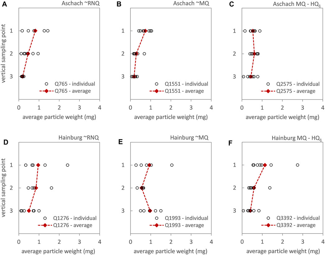
Figure 4. Average particle weights (mg) for microplastics at different characteristic discharges at the study sites Aschach (A–C) and Hainburg (D–F)–black circles represent individual measurements (averaged from the 250 and 500 μm nets), red rhomboids represent average values per vertical sampling point, excluding outliers.
4.2 Quantification of plastic transport
4.2.1 Spatial distribution and cross-sectional transport of plastics
A thorough assessment of spatial distribution of plastic within the cross-sectional profile is essential for transport calculation, including consideration of the hydraulic and morphological features. Given the notable distinctions between the two study sites, with Aschach situated in the backwater of a hydropower plant and Hainburg representing a free-flowing section, our study involves a comprehensive investigation of the lateral and vertical variability at both sites.
Regarding the vertical variability, we compared scaled plastic concentrations due to the wide range of concentrations across individual measurement points, reaching up to 2.6 mg m−3 for microplastic and 4.4 mg m−3 for total plastics. This involved dividing the concentration of each measurement point
At the backwater reach in Aschach, vertical distribution reveals a distinct stratification of plastic particles across the water column during low and mean water discharge, with most particles concentrated near the water surface (Figures 5A, B). However, during the highest sampled discharge, maximum concentrations were observed in the centre and particularly in the lowest net (Figure 5C). In contrast, the free-flowing section of Hainburg shows a more variable and less stratified vertical distribution of microplastic concentrations, especially during low and mean water flow and likely due to higher flow velocities and turbulence mixing (Figures 5D–F). However, surface samples consistently exhibited the highest concentrations for all discharges. Similar characteristics were observed for total plastic concentrations at both study sites.
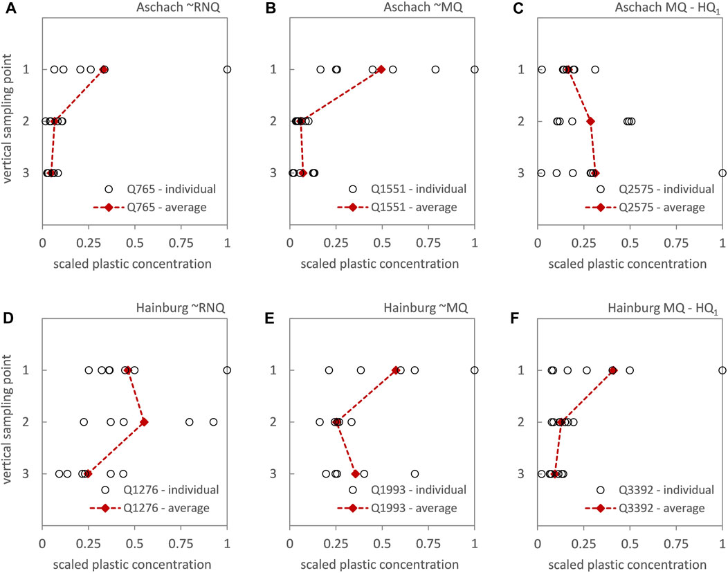
Figure 5. Vertical variability of scaled microplastic concentration at different characteristic discharges at the study sites Aschach (A–C) and Hainburg (D–F)–black circles represent individual measurements (averaged from the 250 and 500 μm nets), red rhomboids represent average values per vertical sampling point.
In terms of lateral variability, we analyzed the depth-averaged concentrations of micro- and total plastics across the measurements at both study sites. While a noticeable increase in concentrations with rising discharge was observed at both sites (Figure 6), differences in lateral distribution, attributed to varying morphological and hydraulic conditions, were observed.
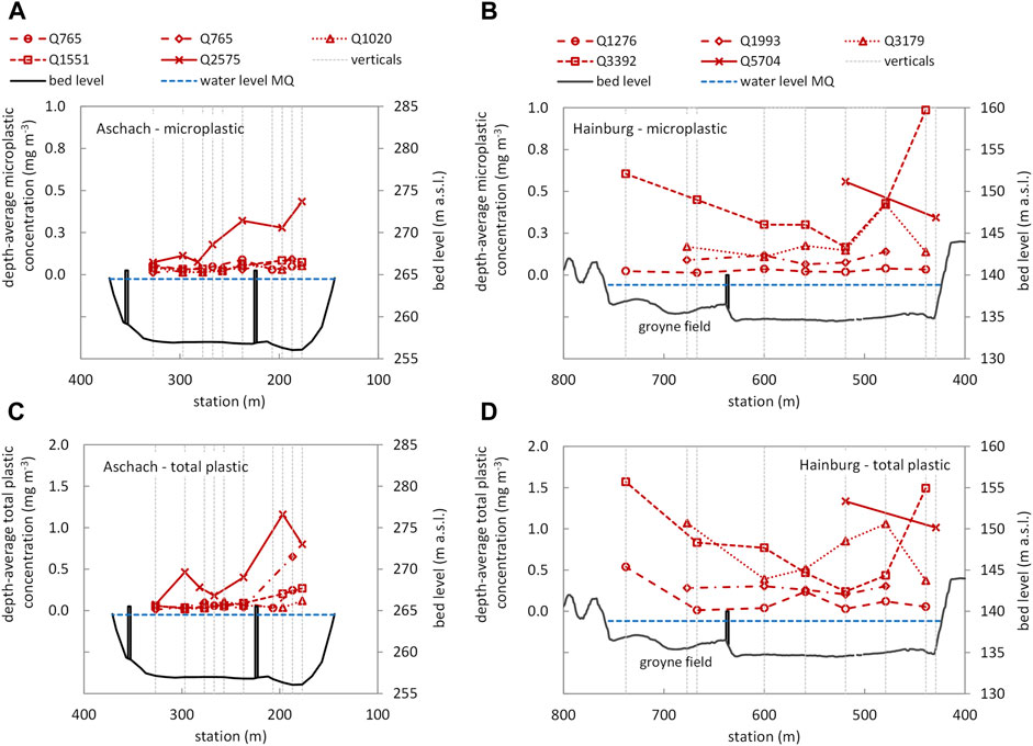
Figure 6. Lateral variability of depth-average plastic concentration during various characteristic discharges at the study sites Aschach (A,C) and Hainburg (B,D)–depicted for microplastic (A,B) and total plastic (C,D)–values of the 250 and 500 μm net were averaged [Data source bed levels Hainburg and annual mean water levels (MQ): via donau].
During low to mean water levels (RNQ–MQ) at both sites, concentrations are evenly distributed across the profile and comparably low for both micro- and total plastics. However, as discharge increases, there is a clear trend of higher concentrations on the right riverbank at the Aschach study site (Figures 6A, C).
In Hainburg, where generally higher characteristic discharges were sampled, a more heterogeneous lateral distribution with increasing discharge levels was noted. Similar to Aschach, a tendency for higher values on the right riverbank compared to the main channel occurred. Additionally, also an increase of concentrations in the left-bank groyne field is visible (Figures 6B, D).
The significant vertical and lateral variabilities observed underline the importance for utilizing cross-sectional multi-point measurements and appropriate spatial integration methods to accurately assess riverine plastic transport. In applying these suggested method, we determined the weighted average concentration
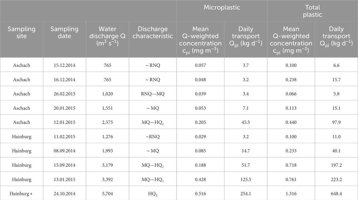
Table 1. Overview of results from direct cross-sectional multi-point net measurements at the Austrian Danube River near Aschach and Hainburg–sorted by study site and discharge, *only two verticals were sampled.
At both study sites, a clear trend of increasing plastic concentration with rising discharge levels is evident. For instance, at the Hainburg study site, during periods of low flow (RNQ), minimum concentrations were recorded at 0.029 mg m−3 for micro- and 0.100 mg m−3 for total plastics, rising up to 0.516 and 1.316 mg m−3 during flood discharge (HQ2) respectively.
Comparing the study sites, plastic transport is similar at low flow (RNQ), ranging from 3.2 to 3.7 kg d−1 in Aschach compared to 3.2 kg d−1 in Hainburg for microplastic. For total plastic, values between 6.6 and 15.7 kg d−1 in Aschach compared to 11.0 kg d−1 in Hainburg were recorded. Plastic transport then increases as a product of both increased concentrations and discharge at both sites. However, with values around and above MQ being two to three times higher for Hainburg (ranging from 14.7 to 125.5 kg d−1 for microplastic and 40.1–232.2 kg d−1 for total plastic) compared to Aschach (ranging from 7.1 to 45.5 kg d−1 and 15.1–97.9 kg d−1 for micro- and total plastic respectively).
4.2.1.1 Evaluation of potential errors due to different monitoring strategies
In this study, we aimed to highlight potential errors in flux determination as a function of input values, comparing (i) the suggested mean discharge-weighted cross-sectional plastic concentration
While at the Aschach study site maximum deviations reaching over +600% were observed during low flow measurements when considering near-bank sampling (white columns in Figures 7A, B), maximum deviations in Hainburg occurred during high water levels (+500% at Q3392 m3s−1) (white columns in Figures 7C, D). In contrast, for a comparable discharge of 3,179 m3s−1 in Hainburg, even a reduction in concentration and transport of −40% was evident compared to the cross-sectional approach, corresponding with findings from the highest sampled discharge at Aschach (−32% at Q2575 m3s−1). Comparing the results when considering near-surface sampling, increased values were observed for most discharges and both study sites, with maximum errors of +152% at Aschach and +70% at Hainburg.
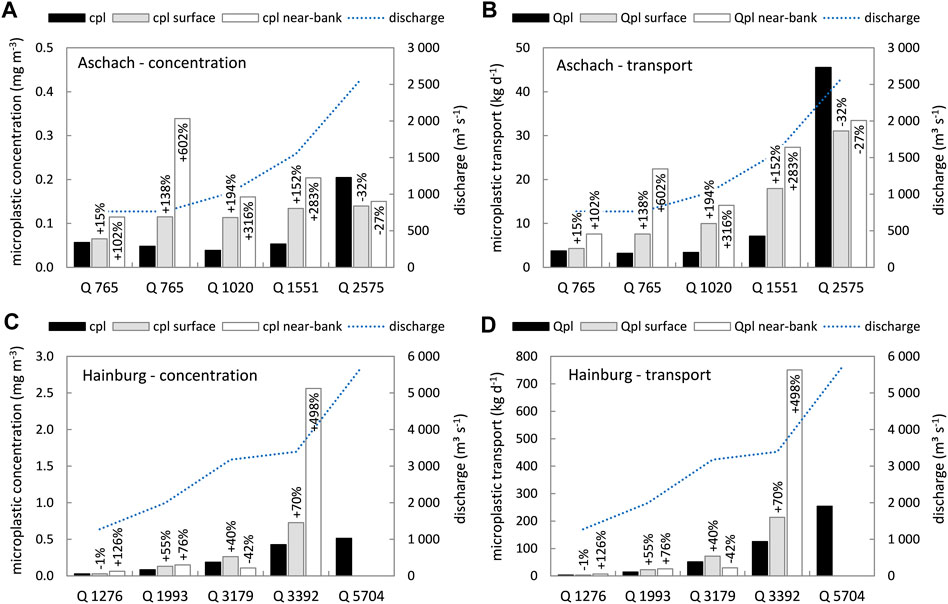
Figure 7. Evaluation of errors using different input values of plastic concentration for transport calculation at the study sites Aschach (A,B) and Hainburg (C,D)–mean discharge-weighted cross-sectional plastic concentration (
Overall, significant deviations are observed when solely relying on near-bank or near-surface samples, with higher errors when using exclusive near-bank samples. While mainly overestimation was observed, no clear discharge-dependent pattern was found. Particularly, the results for near-bank sampling, based on only a single sample, behaved more randomly. Due to their substantial sensitivity to spatial variability associated with considerable scattering of values, significant uncertainties compared to a multi-point measurement are given.
4.2.2 Temporal and discharge dependent distribution of plastics
4.2.2.1 Rating curves and load calculation
Rating curves correlating the daily plastic transport of the cross-sectional measurements with discharge at both study sites were established, both for microplastic and total plastic (Figure 8). For Hainburg, (i) a power function (dashed blue line), (ii) a polynomial function (solid red line) and (iii) a sigmoid function (dash-dotted green line) were fitted to the data points. For Aschach the sigmoid function was not applicable due to missing flood measurements.
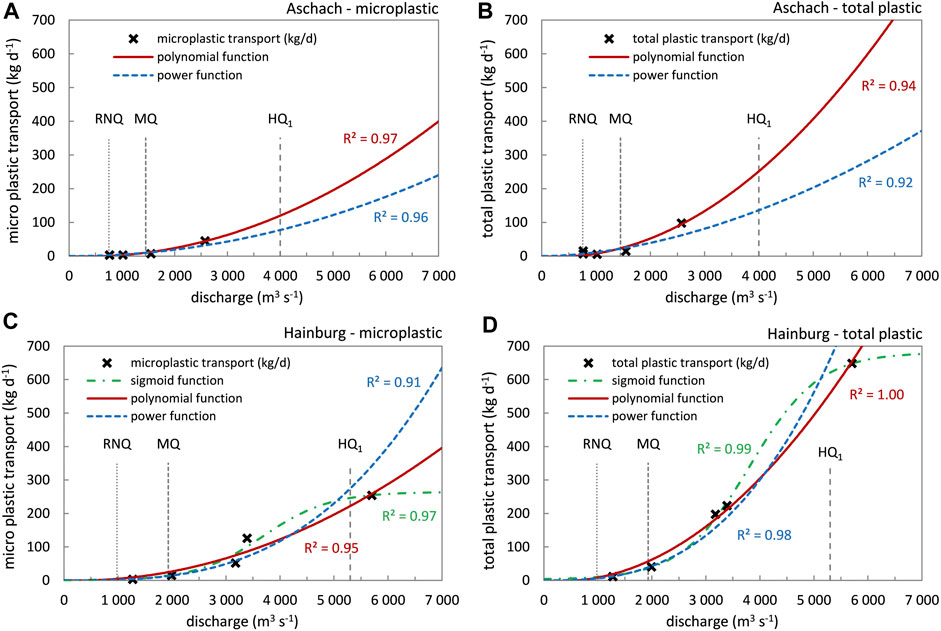
Figure 8. Established rating curves between discharge and daily plastic transport at the study sites Aschach (A,B) and Hainburg (C,D) for microplastic (A,C) and total plastic transport (B,D)–power function (dashed blue line), polynomial function (continuous red line) and sigmoid function (dash-dotted green line)–characteristic discharges for low water level (RNQ), mean water level (MQ) and the 1-year flood event (HQ1) are displayed as vertical lines.
At the Hainburg study site (Figures 8C, D), the power function accurately represents the (more frequently measured) lower transport values but tends to overestimate the transport at higher discharges, while the polynomial function compensates for this effect by slightly overestimating the lower transport values. Both functions have no upper limit, which is remedied by adapting a sigmoid function. For Aschach (Figures 8A, B) the power and polynomial functions show opposite behaviour and, due to missing flood-related data, an increasing range of uncertainty for higher discharges. Overall, the coefficient of determination (R2) for all functions consistently exceeds 0.91.
To comprehend the temporal dynamics of plastic transport in the Danube River, exceedance duration curves correlating plastic transport with duration for the period from 2009 to 2014 were generated through sorting and cumulating plastic transport values. By applying the established rating curves, we determined the temporal variability in plastic transport. Analyzing both microplastic and total plastic and considering the used mathematical functions (power, polynomial and sigmoid), we observed that 50% of the annual plastic load in Aschach is transported within 16% (±5) of the time, with 90% transported within 63% (±10) of the time (Figure 9A). In contrast, at Hainburg, the same proportions of the annual transport occur in 9% (±5) and 55% (±9) of the time, respectively (Figure 9B). Referring to hydrology we discovered that discharges exceeding MQ, which occurred at around 36% of the time at both sites, were responsible for transporting 72% (±8) of the plastic load in Aschach and 81% (±6) in Hainburg. In summary, the temporal transport patterns of plastic in Hainburg are slightly more episodic, with similar amounts of transport occurring within a shorter timeframe compared to Aschach.
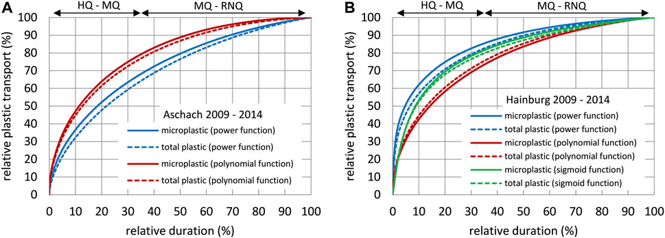
Figure 9. Relative plastic transport related to relative duration for the period 2009 to 2014 at the study sites Aschach (A) and Hainburg (B) for microplastic (continuous lines) and total plastic transport (dashed lines)–power function (blue), polynomial function (red) and sigmoid function (green)–discharge ranges between low and mean flow (RNQ—MQ) as well as mean flow and the flood discharge (MQ—HQ) are marked at the top of the graph.
As long-term plastic loads are critical parameters, annual micro- and total plastic loads were determined using 15-min interval high-resolution hydrological data from nearby gauging stations in Hainburg and Aschach from 2009 to 2014. To evaluate the annual loads in relation to the hydrological conditions, the relative deviations of mean annual flow from the characteristic MQ-discharge for both sites were evaluated, revealing only minor deviations from the characteristic MQ-discharge over the whole period (Aschach: 1,390 m3s−1/-4%, Hainburg: 1900 m3s−1/−1%). However, individual years exhibited deviations of up to ±20%, reflecting both flood- and drought-dominated years as depicted in Figure 10A.
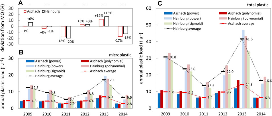
Figure 10. (A) Relative deviation of average annual discharge from mean water discharge (MQ) at the study sites Aschach (red) and Hainburg (black) for the period 2009 to 2014 and (B) calculated annual loads of microplastic and (C) total plastic at both study sites.
In applying the fitted mathematical functions, a range of annual transport loads was calculated. Depending on the rating curve used (power—blue, polynomial–red, sigmoid -green) together with the prevailing hydrology of each year, we observed deviations of up to ±20% (Figures 10B, C). Higher deviations were found in flood-dominated years, where increased uncertainties during extrapolation are evident. As described, the respective functions tend to over- or underestimating partially, thus we averaged the values for further evaluation. When averaged, the mean annual microplastic transport ranged between 2.8 and 6.9 t a−1 (with an average of ⌀4.3 t a−1 for the whole period 2009–2014) at Aschach and from 5.4 to 17.1 t a−1 (⌀10.0) in Hainburg respectively (Figure 10B). Similarly, the total plastic load averaged between 6.3 and 14.3 t a−1 (⌀9.4) at Aschach and from 13.5 to 41.6 t a−1 (⌀24.7) at Hainburg respectively (Figure 10C).
Comparing the annual loads of both sites, Hainburg exhibited 1.9 to 2.7 (⌀2.3) times higher loads for microplastic and 2.1 to 3.1 (⌀2.6) times higher loads for total plastic than Aschach, showing similar characteristics for both size ranges. The plastic load was consequently found to be doubled to tripled within the Austrian section of the Danube River. Microplastic comprised between 36% and 53% (⌀43%) of the total plastic load at Aschach and between 32% and 48% (⌀38%) at Hainburg.
Overall, the annual loads display substantial temporal variability and sensitivity to flood-dominated years. For example, in 2013, with a 12% and 16% increase in mean annual discharge at Aschach and Hainburg, respectively, along with a HQ300 flood event, plastic loads increased by 60% and 53% for micro- and total plastic at Aschach and even higher at Hainburg (71% and 68%) compared to the average transport for 2009 to 2014.
4.2.2.2 Effective discharge
A more detailed understanding of discharge-dependent transport patterns is provided through the effective discharge analysis. Considering all utilized rating curves, the discharge increment transporting most microplastics peaked between 1,500 and 1,650 m3s−1 in Aschach (Figure 11A) and between 2,100 and 2,650 m3s−1 in Hainburg (Figure 11B). At both sites, therefore, the values slightly exceed the MQ-discharge, with a slightly higher sensitivity to flood events at Hainburg. Simultaneously, 50% of the transport occurs at discharges below 1,750 to 2,050 m3s−1 in Aschach and below 2650 to 3,550 m3s−1 in Hainburg. Similar characteristics and values for total plastic transport were observed at both study sites.
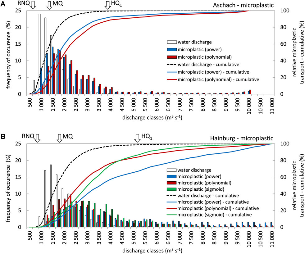
Figure 11. Effective discharge for microplastic transport at the study sites (A) Aschach and (B) Hainburg based on occurrence frequency–power function (blue), polynomial function (red) and sigmoid function (green)–characteristic discharges for low water level (RNQ), mean water level (MQ) and the 1-year flood event (HQ1) are marked at the top of the graph.
5 Discussion
Research on riverine plastic transport has led to the development of various monitoring and sampling techniques, due to the diverse physical properties of plastics and their presence in all types of aquatic environments (Skalska et al., 2020; Lofty et al., 2023; Range et al., 2023). Numerous studies have emphasized the significance of addressing spatio-temporal variations in flowing water when investigating riverine plastics (Liedermann et al., 2018; Mani and Burkhardt-Holm, 2020; Haberstroh et al., 2021; Blondel and Buschman, 2022; Treilles et al., 2022; Skalska et al., 2020; Range et al., 2023). However, approaches for incorporating these variations into flux determination are insufficiently addressed in literature. Therefore, we (i) present a conclusive methodology adapted from sediment research (Edwards and Glysson, 1999; BMLFUW, 2017) aiming to serve as a standard methodology for addressing plastic transport dynamics, (ii) calculate annual loads, and (iii) highlight errors resulting from neglecting spatio-temporal variabilities.
5.1 Methodology for quantification of plastic transport
Spatial integration necessitates addressing plastic across the entire cross-section in conducting multi-point measurements. However, our methodology reveals that, like in sediment research (Edwards and Glysson, 1999), measuring hydraulic conditions by assessing the flow field is essential. Only then, mean discharge-weighted cross-sectional plastic concentration and transport can be accurately computed.
Given the significant role of hydrology in plastic transport dynamics (Liedermann et al., 2018; van Emmerik et al., 2022a), we suggest establishing rating curves between water discharge and plastic transport for temporal integration and annual flux determination, reflecting common practices in sediment research (Walling, 1977; Wass and Leeks, 1999; Asselman, 2000; Horowitz, 2003). In doing so, robust correlations and significant discharge-dependency of plastic transport were observed. The utilization of high-resolution hydrograph data furthermore enables to examine temporal and long-term transport characteristics. Plastic availability, however, can also have a major influence on the relationship between discharge and transport. For example, plastic sources, weir controls at impoundments or other morphological features can lead to discontinuities in the functions and need to be addressed depending on the prevailing boundary conditions. Furthermore, uncertainties may persist regarding potential seasonal effects and the extent of discharge ranges covered. Improved correlations require additional data acquisition.
Based on the findings presented above, we propose that the suggested methodology for quantification of plastic transport is applicable regardless of the underlying sampling methodology—either net sampling, pump sampling or combined approaches. Thereby, as long as isokinetic sampling is employed and the sampling strategy via multi-point sampling appropriately addresses spatio-temporal variabilities and hydraulic conditions during measurement, the methodology can be effectively implemented.
However, limitations of the measurement technique itself need to be considered regarding the size class covered. Net-based sampling devices usually neglect particles smaller than 250 μm. To address this, a combined approach using both net-based devices and pump sampling is suggested for future studies focusing on microplastics. Regarding larger size fractions, our study revealed that adequately addressing rarely found large macroplastics with net-based devices would require longer measurement times and/or increased inlet openings. Since this is often not feasible, we suggest combining alternative approaches for large macroplastics, such as GPS-tracking, counting from bridges, or automated camera systems, as described in the literature (González-Fernández and Hanke, 2017; van Emmerik et al., 2018; Tramoy et al., 2020; van Lieshout et al., 2020).
5.2 Correlation of particle number and mass
Many studies exhibit shortcomings from solely focussing on qualitative aspects or rely on item numbers rather than mass transport, leading to potential over- or underestimation of plastic fluxes (Skalska et al., 2020; Range et al., 2023). To address this, we investigated the particle number to mass ratio of microplastics. Opting for a simplified correlation approach compared to previous methodologies (Kooi and Koelmans, 2019; Koelmans et al., 2020; Range et al., 2023), our analysis aims to support interpreting data from studies lacking mass determination.
We found the average weight of microplastic particles to be 0.63 mg at Aschach and slightly higher but comparable with 0.78 mg at Hainburg. However, individual measurements featured significant variabilities, ranging from 0.06 to more than 6.00 mg per particle. Additionally, we observed more heterogeneous vertical variations in particle masses in the free-flowing section. Heavier particles were predominantly present at the surface layer across all measurements, particularly noticeable under low turbulent conditions. This suggests that larger mass particles rather remain buoyant and float on the surface due to their low density.
5.3 Spatial distribution of plastics
Regarding the vertical distribution, the hydro-morphological characteristics and especially the influence of the downstream hydropower plant induced a pronounced stratification of plastic particles during low and mean water discharge levels at Aschach. In contrast, Hainburg exhibited a more variable and less stratified distribution, likely due to higher flow velocities and turbulence, as well as potential factors such as different polymer densities, aggregation, or biofilm growth, as reported by other authors. Nevertheless, surface nets consistently recorded the highest concentrations at both locations, regardless of discharge levels and consistent with findings by Eo et al. (2019) and Haberstroh et al. (2021). Plastic particles were encountered throughout the river profile and across the entire water column, indicating properties of both suspended and floating matter, therefore.
Regarding lateral distributions, uniform concentrations were observed at both study sites during low to mean water levels. However, as discharge increased, a clear trend of rising plastic concentration emerged, along with distinct lateral patterns, particularly evident in Hainburg. Higher concentrations were observed on the right riverbank at both sites and in the left-bank groyne field at Hainburg. Comparable lateral patterns were reported by Blondel and Buschman (2022) using a similar measurement setup on the Rhine River.
Mean discharge weighted cross-sectional concentrations ranged from 0.029 mg m−3 to 1.316 mg m−3 encompassing all micro- and total plastic measurements at both study sites. Individual samples, however, experienced much higher values reaching up to 2.6 mg m−3 for microplastics and 4.4 mg m−3 for total plastics, consistent with findings from other recent studies (e.g., Haberstroh et al., 2021; Blondel and Buschman, 2022). Consequently, the significant vertical and lateral variabilities observed underscore the importance of conducting cross-sectional multi-point measurements and employing appropriate spatial integration methods for a robust assessment of riverine plastic transport.
5.4 Cross-sectional transport and evaluation of potential errors
Plastic transport was quantified using the suggested methodology for spatial integration. During low flow (RNQ), plastic transport ranged around 3.5 kg d−1 for microplastics and between 6.6 and 15.7 kg d−1 for total plastics at both study sites. Around and above mean flow (MQ), a clear trend of increased transport was observed at both sites, with values being 2–3 times higher at Hainburg compared to Aschach. Microplastic transport ranged from 14.7 to 125.5 kg d−1, and total plastic transport from 40.1 to 232.2 kg d−1 at Hainburg, compared to 7.1–45.5 kg d−1 for microplastics and 15.1–97.9 kg d−1 for total plastics in Aschach.
Assessing potential errors in load calculation highlighted the importance of cross-sectional multi-point measurements for accurate plastic transport assessment. Significant deviations were observed when considering only near-bank or near-surface samples, with even higher errors exceeding +600% when exclusively considering near-bank sampling. While overestimation was common, no clear discharge-dependent pattern was found, particularly for near-bank sampling. Depending solely on a single sample may thus lead to a significant overestimation or underestimation of plastic transport, given the considerable spatial variability in plastic distribution within the cross-section.
Thus, based on our data, we consider that an average daily transport near Hainburg of approximately 338 kg d−1, as published by Lechner et al. (2014), is notably overestimating, as their sampling was limited to the shoreline and overlooking spatio-temporal aspects. Our findings are furthermore supported by results from Eo et al. (2019) for the Nakdong River in South Korea, where 2–3 times higher annual loads were computed when only addressing surface sampling.
5.5 Temporal and discharge-dependent transport
Analysis of temporal and discharge-dependent distribution patterns involved establishing rating curves utilizing high-resolution hydrograph data. We found, that 50% of the annual plastic load was transported within 16% (±5) of time in Aschach, compared to only 9% (±5) at the Hainburg study site. Referring to hydrology, discharges exceeding MQ, observed approximately 36% of the time at both sites, were responsible for transporting 72% (±8) of the plastic load in Aschach and 81% (±6) in Hainburg, exhibiting slightly more episodic behaviour. Effective discharge was found slightly above the mean discharge at both sites, with moderately higher sensitivity to flood events at Hainburg. However, unlike sediment research, where effective discharge typically is associated with recurrence intervals of 1–2 years and corresponds to the bankfull discharge (Wolman and Miller, 1960; Andrews, 1980; Pessenlehner et al., 2022), a moderate discharge dependency of plastic transport can be inferred.
5.6 Load calculation
Overall, microplastics accounted for 32%–53% of the total transport. The mean annual microplastic transport ranged between 2.8 and 6.9 t a−1 (with an average of ⌀4.3 t a−1 for the whole period 2009–2014) in Aschach and from 5.4 to 17.1 t a−1 (⌀10.0) in Hainburg. Similarly, the total plastic load averaged between 6.3 and 14.3 t a−1 (⌀9.4) in Aschach and from 13.5 to 41.6 t a−1 (⌀24.7) in Hainburg. Comparing the annual loads of both sites, the plastic load was therefore found to be doubled to tripled within the Austrian section of the Danube River. At the same time this increase in plastic transport compares to an only 33% rise in both catchment size and mean water discharge between the two sampling locations.
In contrast to findings in tidal zones where rivers are rather described as temporary sinks and reservoirs for plastic pollution, diverting only a low percentage of plastic waste to the sea (Meijer et al., 2021; van Emmerik et al., 2022b; van Emmerik et al., 2023), our study reveals different characteristics. We observed a clear longitudinal increase in plastic transport, however, relating to a comparably steeper river section in an upstream catchment featuring different hydro-morphological characteristics. Yet, the correlation between rising discharge and both enhanced plastic concentration and transport rates comprised within our study indicates their widespread occurrence in the river systems. Like in sediment research, we therefore consider that rivers can simultaneously function as source, pathway and sink at the same time, depending on the prevailing hydro-morphological boundary conditions.
To enhance our understanding of riverine plastic transport, it is crucial to consider hydrological boundary conditions, morphological features, lateral structures such as hydropower plants and the entire journey of plastics from their source to the sea. We therefore encourage longitudinal, basin-wide assessments of plastic transport using appropriate monitoring techniques to adequately address spatial, temporal, and discharge-induced variabilities. Only through a solid understanding of riverine plastic transport and reliable data, plastic sources can be identified to assign responsibilities for plastic pollution. Furthermore, mitigation measures and cleaning actions will benefit and can be applied more effectively to remove plastic from river catchments and prevent it from entering the oceans.
Data availability statement
The raw data supporting the conclusions of this article will be made available by the authors, without undue reservation.
Author contributions
SP: Conceptualization, Data curation, Formal Analysis, Investigation, Methodology, Validation, Visualization, Writing–original draft, Writing–review and editing. PG: Conceptualization, Data curation, Formal Analysis, Investigation, Methodology, Validation, Visualization, Writing–review and editing, Writing–original draft. HH: Conceptualization, Funding acquisition, Methodology, Project administration, Resources, Supervision, Writing–original draft, Writing–review and editing. ML: Conceptualization, Funding acquisition, Investigation, Methodology, Project administration, Resources, Supervision, Validation, Writing–original draft, Writing–review and editing.
Funding
The author(s) declare that financial support was received for the research, authorship, and/or publication of this article. The study is supported by the project “Microplastics at the Danube” funded by the Federal Ministry BML (formally called BMLFUW) and the authorities of Lower Austria, Upper Austria and Vienna. The financial support by the Austrian Federal Ministry of Labour and Economy, the National Foundation for Research, Technology and Development and the Christian Doppler Research Association is gratefully acknowledged.
Acknowledgments
The project “Microplastics at the Danube” was coordinated by the Environment Agency Austria and implemented with the help of via donau. The authors want to thank Marlene Haimann, Barbara Weidenhiller, Martin Hinterleitner, Nicolas Fischer, Michael Krapesch and Marton Szinetar for their help during field work and sample analysis.
Conflict of interest
The authors declare that the research was conducted in the absence of any commercial or financial relationships that could be construed as a potential conflict of interest.
Publisher’s note
All claims expressed in this article are solely those of the authors and do not necessarily represent those of their affiliated organizations, or those of the publisher, the editors and the reviewers. Any product that may be evaluated in this article, or claim that may be made by its manufacturer, is not guaranteed or endorsed by the publisher.
References
Allen, S., Allen, D., Phoenix, V. R., Le Roux, G., Durántez Jiménez, P., Simonneau, A., et al. (2019). Atmospheric transport and deposition of microplastics in a remote mountain catchment. Nat. Geosci. 12 (5), 339–344. doi:10.1038/s41561-019-0335-5
Anderson, J. C., Park, B. J., and Palace, V. P. (2016). Microplastics in aquatic environments: implications for Canadian ecosystems. Environ. Pollut. 218, 269–280. doi:10.1016/j.envpol.2016.06.074
Andrews, E. D. (1980). Effective and bankfull discharges of streams in the Yampa River basin, Colorado and Wyoming. J. Hydrology 46 (3-4), 311–330. doi:10.1016/0022−1694(80)90084-0
Asselman, N. E. M. (2000). Fitting and interpretation of sediment rating curves. J. Hydrology 234 (3-4), 228–248. doi:10.1016/S0022−1694(00)00253-5
Bakir, A., Rowland, S. J., and Thompson, R. C. (2014). Enhanced desorption of persistent organic pollutants from microplastics under simulated physiological conditions. Environ. Pollut. 185, 16–23. doi:10.1016/j.envpol.2013.10.007
Blondel, E., and Buschman, F. A. (2022). Vertical and horizontal plastic litter distribution in a bend of a tidal river. Front. Environ. Sci. 10, 861457. doi:10.3389/fenvs.2022.861457
BMLFUW (2017). Schwebstoffe im Fließgewässer-Leitfaden zur Erfassung des Schwebstofftransports. Bundesministerium für Land-und Forstwirtschaft, Umwelt und Wasserwirtschaft, 2. Auflage, Wien. IN GERMAN. Available at: https://www.bmnt.gv.at/wasser/wasser-oesterreich/wasserkreislauf/Schwebstoffe_LF.html.
Boon, A., Buschman, F. A., van Emmerik, T. H., Broere, S., and Vermeulen, B. (2023). Detection of suspended macroplastics using acoustic Doppler current profiler (ADCP) echo. Front. Earth Sci. 11, 1231595. doi:10.3389/feart.2023.1231595
Bordos, G., Gergely, S., Háhn, J., Palotai, Z., Szabó, É., Besenyő, G., et al. (2021). Validation of pressurized fractionated filtration microplastic sampling in controlled test environment. Water Res. 189, 116572. doi:10.1016/j.watres.2020.116572
Broere, S., van Emmerik, T., González-Fernández, D., Luxemburg, W., de Schipper, M., Cózar, A., et al. (2021). Towards underwater macroplastic monitoring using echo sounding. Front. Earth Sci. 9, 628704. doi:10.3389/feart.2021.628704
Cole, M., Lindeque, P., Halsband, C., and Galloway, T. S. (2011). Microplastics as contaminants in the marine environment: a review. Mar. Pollut. Bull. 62 (12), 2588–2597. doi:10.1016/j.marpolbul.2011.09.025
Dris, R., Gasperi, J., Rocher, V., Saad, M., Renault, N., and Tassin, B. (2015). Microplastic contamination in an urban area: a case study in Greater Paris. Environ. Chem. 12 (5), 592–599. doi:10.1071/EN14167
Edwards, T., and Glysson, G. (1999). “Field methods for measurement of fluvial sediment,” in Techniques of water-resources investigations of the U.S. Geological survey, book 3, application of hydraulics (Washington, DC, USA: United States Government Printing Office), 89. Chapter C2.
Eo, S., Hong, S. H., Song, Y. K., Han, G. M., and Shim, W. J. (2019). Spatiotemporal distribution and annual load of microplastics in the Nakdong River, South Korea. Water Res. 160, 228–237. doi:10.1016/j.watres.2019.05.053
Geraeds, M., van Emmerik, T., de Vries, R., and bin Ab Razak, M. S. (2019). Riverine plastic litter monitoring using unmanned aerial vehicles (UAVs). Remote Sens. 11 (17), 2045. doi:10.3390/rs11172045
González-Fernández, D., and Hanke, G. (2017). Toward a harmonized approach for monitoring of riverine floating macro litter inputs to the marine environment. Front. Mar. Sci. 4, 86. doi:10.3389/fmars.2017.00086
Haberstroh, C. J., Arias, M. E., Yin, Z., and Wang, M. C. (2021). Effects of hydrodynamics on the cross-sectional distribution and transport of plastic in an urban coastal river. Water Environ. Res. 93 (2), 186–200. doi:10.1002/wer.1386
Haimann, M., Liedermann, M., Lalk, P., and Habersack, H. (2014). An integrated suspended sediment transport monitoring and analysis concept. Int. J. Sediment Res. 29 (2), 135–148. doi:10.1016/S1001-6279(14)60030-5
Hartmann, N. B., Hüffer, T., Thompson, R. C., Hassellov, M., Verschoor, A., Daugaard, A. E., et al. (2019). Are we speaking the same language? Recommendations for a definition and categorization framework for plastic debris. Environ. Sci. and Technol. 53, 1039–1047. doi:10.1021/acs.est.8b05297
Hermabessiere, L., Dehaut, A., Paul-Pont, I., Lacroix, C., Jezequel, R., Soudant, P., et al. (2017). Occurrence and effects of plastic additives on marine environments and organisms: a review. Chemosphere 182, 781–793. doi:10.1016/j.chemosphere.2017.05.096
Hohenblum, P., Liebmann, B., and Liedermann, M. (2015). Plastic and microplastic in the environment (REP-0551, umweltbundesamt, 2015).
Horowitz, A. J. (2003). An evaluation of sediment rating curves for estimating suspended sediment concentrations for subsequent flux calculations. Hydrol. Process. 17 (17), 3387–3409. doi:10.1002/hyp.1299
ICPDR (2015). The Danube River Basin District management plan—Part A—basin-Wide Overview. Vienna, Austria: International Commission for the Protection of the Danube River, 192.
ISO 4363 (2002). Measurement of liquid flow in open channels-methods for measurement of characteristics of suspended sediment. Geneva, Switzerland: International Standard.
Koelmans, A. A., Redondo-Hasselerharm, P. E., Mohamed Nor, N. H., and Kooi, M. (2020). Solving the nonalignment of methods and approaches used in microplastic research to consistently characterize risk. Environ. Sci. and Technol. 54 (19), 12307–12315. doi:10.1021/acs.est.0c02982
Kondolf, G. M. (1997). PROFILE: hungry water: effects of dams and gravel mining on river channels. Environ. Manag. 21 (4), 533–551. doi:10.1007/s002679900048
Kooi, M., and Koelmans, A. A. (2019). Simplifying microplastic via continuous probability distributions for size, shape, and density. Environ. Sci. and Technol. Lett. 6 (9), 551–557. doi:10.1021/acs.estlett.9b00379
Lebreton, L. C., Van Der Zwet, J., Damsteeg, J. W., Slat, B., Andrady, A., and Reisser, J. (2017). River plastic emissions to the world’s oceans. Nat. Commun. 8 (1), 15611. doi:10.1038/ncomms15611
Lechner, A., Keckeis, H., Lumesberger-Loisl, F., Zens, B., Krusch, R., Tritthart, M., et al. (2014). The Danube so colourful: a potpourri of plastic litter outnumbers fish larvae in Europe's second largest river. Environ. Pollut. 188, 177–181. doi:10.1016/j.envpol.2014.02.006
Lenaker, P. L., Baldwin, A. K., Corsi, S. R., Mason, S. A., Reneau, P. C., and Scott, J. W. (2019). Vertical distribution of microplastics in the water column and surficial sediment from the Milwaukee River Basin to lake Michigan. Environ. Sci. and Technol. 53, 12227–12237. doi:10.1021/acs.est.9b03850
Liedermann, M., Gmeiner, P., Kreisler, A., Tritthart, M., and Habersack, H. (2017). Insights into bedload transport processes of a large regulated gravel-bed river. Earth Surf. Process. Landforms 43 (2), 514–523. doi:10.1002/esp.4253
Liedermann, M., Gmeiner, P., Pessenlehner, S., Haimann, M., Hohenblum, P., and Habersack, H. (2018). A methodology for measuring microplastic transport in large or medium rivers. Water 10 (4), 414. doi:10.3390/w10040414
Lofty, J., Ouro, P., and Wilson, C. A. M. E. (2023). Microplastics in the riverine environment: meta-analysis and quality criteria for developing robust field sampling procedures. Sci. Total Environ. 863, 160893. doi:10.1016/j.scitotenv.2022.160893
Mani, T., and Burkhardt-Holm, P. (2020). Seasonal microplastics variation in nival and pluvial stretches of the Rhine River–From the Swiss catchment towards the North Sea. Sci. Total Environ. 707, 135579. doi:10.1016/j.scitotenv.2019.135579
Meijer, L. J., Van Emmerik, T., Van Der Ent, R., Schmidt, C., and Lebreton, L. (2021). More than 1000 rivers account for 80% of global riverine plastic emissions into the ocean. Sci. Adv. 7 (18), eaaz5803. doi:10.1126/sciadv.aaz5803
Mohsen, A., Kovács, F., and Kiss, T. (2023). Riverine microplastic quantification: a novel approach integrating satellite images, neural network, and suspended sediment data as a proxy. Sensors 23 (23), 9505. doi:10.3390/s23239505
Pessenlehner, S., Liedermann, M., Holzapfel, P., Skrame, K., Habersack, H., and Hauer, C. (2022). Evaluation of hydropower projects in Balkan Rivers based on direct sediment transport measurements; challenges, limits and possible data interpretation—case study Vjosa River/Albania. River Res. Appl. 38 (6), 1014–1030. doi:10.1002/rra.3979
Prata, J. C., Da Costa, J. P., Duarte, A. C., and Rocha-Santos, T. (2019). Methods for sampling and detection of microplastics in water and sediment: a critical review. Trends Anal. Chem. 110, 150–159. doi:10.1016/j.trac.2018.10.029
Range, D., Scherer, C., Stock, F., Ternes, T., and Hoffmann, T. (2023). Hydro-geomorphic perspectives on microplastic distribution in freshwater river systems: a critical review. Water Res. 245 (1), 120567. doi:10.1016/j.watres.2023.120567
Skalska, K., Ockelford, A., Ebdon, J. E., and Cundy, A. B. (2020). Riverine microplastics: behaviour, spatio-temporal variability, and recommendations for standardised sampling and monitoring. J. Water Process Eng. 38, 101600. doi:10.1016/j.jwpe.2020.101600
Stock, F., Kochleus, C., Bänsch-Baltruschat, B., Brennholt, N., and Reifferscheid, G. (2019). Sampling techniques and preparation methods for microplastic analyses in the aquatic environment–A review. Trends Anal. Chem. 113, 84–92. doi:10.1016/j.trac.2019.01.014
Tramoy, R., Gasperi, J., Colasse, L., Silvestre, M., Dubois, P., Noûs, C., et al. (2020). Transfer dynamics of macroplastics in estuaries—New insights from the seine estuary: Part 2. Short-term dynamics based on GPS-trackers. Mar. Pollut. Bull. 160, 111566. doi:10.1016/j.marpolbul.2020.111566
Treilles, R., Gasperi, J., Tramoy, R., Dris, R., Gallard, A., Partibane, C., et al. (2022). Microplastic and microfiber fluxes in the Seine River: flood events versus dry periods. Sci. Total Environ. 805, 150123. doi:10.1016/j.scitotenv.2021.150123
van Emmerik, T., de Lange, S., Frings, R., Schreyers, L., Aalderink, H., Leusink, J., et al. (2022a). Hydrology as a driver of floating river plastic transport. Earth’sFuture 10, e2022EF002811. doi:10.1029/2022EF002811
van Emmerik, T., Kieu-Le, T.-C., Loozen, M., Oeveren, K., Strady, E., Bui, X.-T., et al. (2018). A methodology to characterize riverine macroplastic emission into the ocean. Front. Mar. Sci. 5. doi:10.3389/fmars.2018.00372
Van Emmerik, T., Mellink, Y., Hauk, R., Waldschläger, K., and Schreyers, L. (2022b). Rivers as plastic reservoirs. Front. Water 3, 786936. doi:10.3389/frwa.2021.786936
van Emmerik, T., and Schwarz, A. (2020). Plastic debris in rivers. Wiley Interdiscip. Rev. Water 7 (1), e1398. doi:10.1002/wat2.1398
van Emmerik, T. H., Frings, R. M., Schreyers, L. J., Hauk, R., de Lange, S. I., and Mellink, Y. A. (2023). River plastic transport and deposition amplified by extreme flood. Nat. Water 1 (6), 514–522. doi:10.1038/s44221-023-00092-7
van Lieshout, C., van Oeveren, K., van Emmerik, T., and Postma, E. (2020). Automated River plastic monitoring using deep learning and cameras. Earth Space Sci. 7 (8). doi:10.1029/2019EA000960
via donau (2012). Die kennzeichnenden Wasserstände der österreichischen Donau–KWD 2010. via donau Österreichische Wasserstraßen-Gesellschaft mbH. Donau-City-Straße, 1220 Wien.
Waldschlager, K., and Schuttrumpf, H. (2019). Effects of particle properties on the settling and rise velocities of microplastics in freshwater under laboratory conditions. Environ. Sci. and Technol. 53 (4), 1958–1966. doi:10.1021/acs.est.8b06794
Walling, D. E. (1977). Assessing the accuracy of suspended sediment rating curves for a small basin. Water Resour. Res. 13 (3), 531–538. doi:10.1029/WR013i003p00531
Wass, P. D., and Leeks, G. J. (1999). Suspended sediment fluxes in the Humber catchment, UK. Hydrol. Process. 13 (7), 935–953. doi:10.1002/(SICI)1099−1085(199905)13:7<935::AID-HYP783>3.0.CO;2-L
Wolman, M. G., and Miller, J. P. (1960). Magnitude and frequency of forces in geomorphic processes. J. Geol. 68 (1), 54–74. doi:10.1086/626637
Woodward, J., Li, J., Rothwell, J., and Hurley, R. (2021). Acute riverine microplastic contamination due to avoidable releases of untreated wastewater. Nat. Sustain. 4 (9), 793–802. doi:10.1038/s41893-021-00718-2
Wright, S. L., Thompson, R. C., and Galloway, T. S. (2013). The physical impacts of microplastics on marine organisms: a review. Environ. Pollut. 178, 483–492. doi:10.1016/j.envpol.2013.02.031
Keywords: direct measurements, multi-point net sampling, riverine plastic transport, spatio-temporal variability, rating curves, plastic flux determination, Danube River
Citation: Pessenlehner S, Gmeiner P, Habersack H and Liedermann M (2024) Understanding the spatio-temporal behaviour of riverine plastic transport and its significance for flux determination: insights from direct measurements in the Austrian Danube River. Front. Earth Sci. 12:1426158. doi: 10.3389/feart.2024.1426158
Received: 30 April 2024; Accepted: 05 August 2024;
Published: 21 August 2024.
Edited by:
Shailesh Kumar Singh, National Institute of Water and Atmospheric Research (NIWA), New ZealandReviewed by:
Pierre Girard, Federal University of Mato Grosso, BrazilKatrin Wendt-Potthoff, Helmholtz Association of German Research Centres (HZ), Germany
Irene Martins, University of Porto, Portugal
Copyright © 2024 Pessenlehner, Gmeiner, Habersack and Liedermann. This is an open-access article distributed under the terms of the Creative Commons Attribution License (CC BY). The use, distribution or reproduction in other forums is permitted, provided the original author(s) and the copyright owner(s) are credited and that the original publication in this journal is cited, in accordance with accepted academic practice. No use, distribution or reproduction is permitted which does not comply with these terms.
*Correspondence: Sebastian Pessenlehner, c2ViYXN0aWFuLnBlc3NlbmxlaG5lckBib2t1LmFjLmF0; Marcel Liedermann, bWFyY2VsLmxpZWRlcm1hbm5AYm9rdS5hYy5hdA==