Meshfree modelling of magnetotelluric and controlled-source electromagnetic data for conductive earth models with complex geometries

Geophysical electromagnetic survey methods are particularly effective in locating conductive mineral deposits or mineralization zones in a mineral resource exploration. The forward modelling of the electromagnetic responses over such targets is a fundamental task in quantitatively interpreting the geophysical data into a geological model. Due to the ubiquitous irregular and complex geometries associated with the mineral rock units, it is critical that the numerical modelling approach being used is able to adequately and efficiently incorporate any necessary geometries of the Earth model. To circumvent the difficulties in representing complex but necessary geometry features in an Earth model for the existing mesh-based numerical modelling approaches (e.g., finite element and finite difference methods), I present a meshfree modelling approach that does not require a mesh to solve the Maxwell’s equations. The meshfree approach utilizes a set of unconnected points to represent any geometries in the Earth model, allowing for the maximal flexibility to account for irregular surface geometries and topography. In each meshfree subdomain, radial basis functions are used to construct meshfree function approximation in transforming the differential equations in the modelling problem into linear systems of equations. The method solves the potential function equations of the Maxwell’s equations in the modelling. The modelling accuracy using the meshfree method is examined and verified using one magnetotelluric model and two frequency-domain controlled-source models. The magnetotelluric model is the well-known Dublin Test Model 2 in which the spherical geometry of the conductor in the shallow subsurface may pose as a challenge for many numerical modelling methods. The first controlled-source model is a simple half-space model with the electric dipole source for which analytical solutions exist for the modelling responses. The second controlled-source model is the volcanic massive sulphide mineral deposit from Voisey’s Bay, Labrador, Canada in which the deposit’s surface is highly irregular. For all modellings, the calculated electromagnetic responses are found to agree with other independent numerical solutions and the analytical solutions. The advantages of the meshfree method in discretizing the Earth models with complex geometries in the forward modelling of geophysical electromagnetic data is clearly demonstrated.

1 Introduction

Geophysical electromagnetic (EM) survey methods continue to be important in the exploration of mineral resources, particularly those with a high conductivity contrast from their host rocks (e.g., copper, zinc, iron, nickle) (Strangway et al., 1973; Dyck and West, 1984; Farquharson and Craven, 2009; Smith, 2014; Gehrmann et al., 2019). In recent years, due to the increasing acknowledgement of the important role of mineral resources in energy transition, various “critical mineral resource” initiatives have been proposed (e.g., Schulz et al., 2017) and how we as a society can meet the demands has sparkled much discussion (Jones, 2023).

A geophysical EM survey directly produces a map of the distribution of electrical conductivity of the subsurface. Naturally, the interpretation of any EM data collected over a region of interest becomes vital in determining the parameters of potential mineral deposits that may host economic resources. At the centre of a quantitative interpretation of EM data is the numerical modelling of EM responses (including controlled-source EM, magnetotelluric, transient EM data) which plays a critical role in the development of theories and methods of various EM survey techniques. Of the various advancements made over the last few decades (e.g., Nabighian, 1988; Zhdanov, 2010; Smith, 2014), the numerical modelling of EM data has steadily evolved from closed-form, analytical computations of EM responses over relatively simple conductivity models that started around 1960s (Wait, 1960; Nabighian, 1988) to fully numerical simulations of Maxwell’s equations over Earth models with complex geometries and nonlinear, anisotropic conductivity distributions nowadays (e.g., Newman, 2014; Han et al., 2018).

The importance of representing realistically complex geometries of conductive mineral deposits or mineralization zones in the EM data modelling becomes obvious since mineral deposits or mineralization zones are naturally of irregular shapes of geometry, with some presenting quite extreme geometries (e.g., uranium deposits associated with thin graphite Zeng et al., 2019; Lu et al., 2021). Despite the ubiquitous existence and importance of such realistic geometries, there are still significant challenges faced by numerical modelling techniques in terms of efficiently incorporating the geometries. These challenges are precisely what this study is trying to solve and in order to do so, a new type of modelling techniques called meshfree methods is used which I will present in detail in the following sections.

Numerical methods of forward modelling EM responses over a general three-dimensional (3-D) conductivity Earth model are often focused on mesh-based modelling methods in the applied geophysics which include finite difference (e.g., Yee, 1966; Taflove and Umashankar, 1990; Mackie et al., 1993; Wang and Hohmann, 1993; Newman and Alumbaugh, 1995; Streich, 2009), finite volume (e.g., Jahandari and Farquharson, 2014; Jahandari et al., 2017), integral equation (e.g., Jones and Pascoe, 1972; Hohmann, 1975; Newman et al., 1986; Farquharson and Oldenburg, 2002; Chen et al., 2021) and finite element methods (e.g., Coggon, 1971; Pridmore et al., 1981; Badea et al., 2001; Nam et al., 2007; Puzyrev et al., 2013; Li J. et al., 2017; Rochlitz et al., 2019). They are termed mesh-based modelling methods in this study because they have the common feature of relying on a mesh-based discretization (e.g., rectilinear, triangular and tetrahedral meshes; see Figure 1A,B) of the conductivity model. Among these mesh-based methods, finite difference approaches may face more challenges than others in accurately representing complex topography surfaces and irregular surface geometries of a conductor since they require tensor-grid function approximation of differential equations. In contrast, finite volume, integral equation and finite element methods do not face such limitation. It may be argued that finite element modelling techniques, if combined with unstructured meshes whose automatic generations are facilitated by modern mesh generation software (Fabri et al., 2000; Si, 2015), are the most flexible mesh-based approaches in the modelling of EM data over complex Earth models (Coggon, 1971; Günther et al., 2006; Nam et al., 2007; Miensopust et al., 2013).

Figure 1

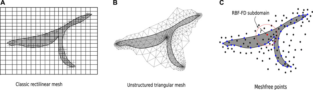
Figure 1. Schematic illustration of model discretizations for 2-D irregular geometries using (A) rectilinear mesh with local quadtree refinements, (B) unstructured triangular mesh and (C) meshfree points. Adapted from Long and Farquharson (2019c).

For real-life geometries of exploration targets, unstructured meshes (e.g., triangular and tetrahedral meshes) possess a unique advantage in efficiently and accurately representing complex geometries that are important characteristics of potential exploration targets (Lelièvre et al., 2012; Lu et al., 2021). However, accurate numerical solution of EM responses using mesh-based modelling techniques, including finite element and finite volume methods, also require a certain degree of regularity of the mesh cells. In the finite element case, for example, the effect of the mesh quality (e.g., the ratio of the largest to smallest cell sizes, elongation, dihedral angles and radius-edge ratio of cells for tetrahedral meshes) on the computational accuracy is demonstrated to be significant (Du et al., 2009). Poor mesh quality can lead to very slow convergence or divergence in iteratively solving the resulting linear system of equations in modelling controlled-source EM data using a vector finite element implementation (Ansari and Farquharson, 2014). On the other hand, ensuring the quality of the mesh can lead to overwhelmingly excessive number of elements in the generated mesh, therefore intractable computational resources, in order to sufficiently conform to the real geometries in the model (Schwarzbach et al., 2011; Nalepa et al., 2016).

The dilemma in balancing the quality of unstructured meshes and the number of mesh cells is often addressed using adaptive mesh refinement techniques (Oden and Prudhomme, 2001; Key and Ovall, 2011; Schwarzbach et al., 2011; Ren et al., 2013; Zhang et al., 2018; Spitzer, 2024). In an adaptive mesh refinement approach, the current mesh used for the modelling of EM responses can be further refined or coarsened based on an estimate of the current numerical modelling error. The ideal result is that only the part of the mesh with the largest numerical errors is refined. In the unstructured mesh scenario, the adaptive refining process is often carried out by locally modifying the mesh, rather than re-meshing the whole Earth model, due to the concern of efficiency and robustness of the process (Zhang et al., 2018; Liu et al., 2023). However, complications may arise during the adaptive mesh refining. First, as the topology of the mesh changes at each refining step the mapping between the old mesh and the new mesh needs to be calculated in order to update the degrees of freedom, which can be an expensive and rather complicated process. Second, further dividing the cells in the current mesh may produce “hanging nodes” due to the non-conforming new cells within the parent cells (Jahandari et al., 2021). The nonconformity of the new mesh may be eliminated at the cost of further refining neighbouring cells, often with a lower quality of the generated new cells.

Alternatively, the Earth model can be discretized using meshfree points (see Figure 1C) and the corresponding numerical modelling techniques are called meshfree methods (Nguyen et al., 2008; Chen et al., 2017). A set of unconnected points, or meshfree points, serve for the same purpose as that of a quality mesh in obtaining an accurate numerical solution in forward modelling the EM data. Because of the lack of connectivity among the points, the physical property distribution (i.e., the conductivity distribution for EM data modelling) will be sampled on the points when discretizing the partial differential equations. With a meshfree point discretization, the density and regularity of the point distribution are still important for accurate numerical modellings; however, the advantages of manipulating points over mesh generations are:

• With comparable regularity of a quality mesh, the generation of points requires much less effort in computer programming and is more straightforward. Also, the development of dedicated point generation software is also significantly easier (Fornberg and Flyer, 2015).

• Since there is no topology requirement, the generation of quality, unstructured meshfree points can be more robust than generating a quality unstructured mesh (Du et al., 2002; Slak and Kosec, 2019).

• Adaptive point refining and/or coarsening is more computationally efficient than the same process when using meshes, since any addition or deletion of local points does not need to affect the rest of the points. The nonconformity issue and its complications in a mesh-based adaptive refining are completely removed (Rabczuk and Belytschko, 2005).

Based on a distribution of points, many meshfree methods for solving partial differential equations have been proposed (Chen et al., 2017). For geophysical data modelling, however, only a few different meshfree methods have been proposed for seismic wave field modelling (e.g., Jia and Hu, 2006; Takekawa et al., 2015; Li B. et al., 2017), gravity data modelling (e.g., Long and Farquharson, 2019c) and EM data modelling (e.g., Wittke and Tezkan, 2014; Long and Farquharson, 2017; Long and Farquharson, 2019a; Long and Farquharson, 2019b). In general, different meshfree methods differ in the choice of basis functions, the types of meshfree points (i.e., uniform or unstructured) and in that whether numerical integration is required in transforming the partial differential equations into the linear system of equations. The meshfree method demonstrated here, mostly known as radial-basis-function based finite difference (RBF-FD), does not need the potentially expensive step of numerical integration. It also naturally supports unstructured point distributions allowing for an efficient discretization of complex-geometry conductivity models. Meshfree modelling of EM data is considered to be more challenging than those of seismic and gravity data since the EM fields are discontinuous across conductivity discontinuities (Long and Farquharson, 2019b).

The rest of the study is organized as follows. The details of the meshfree modelling method in the context of numerically solving Maxwell’s equations will be first presented, which is followed by the demonstration of the numerical accuracy of the method using a magnetotelluric example and two controlled-source EM examples. Further discussions for the applicability for other types of geophysical data of the modelling method are also presented before I conclude the study.

2 Methods

2.1 Maxwell’s equations for meshfree modelling

The frequency-domain Maxwell’s equations for the electromagnetic field in the quasi-static limit are expressed as (Stratton, 2007)

$\nabla \times \mathbf{E}=-i\omega \mathbf{B},(1)$

$\nabla \times \mathbf{H}=\sigma \mathbf{E}+{\mathbf{J}}_{\mathit{exe}},(2)$

for Faraday’s law and Ampère’s law, respectively. Here, $\mathbf{E}$ and $\mathbf{B}$ are the electric field and magnetic induction vector, respectively. $\mathbf{B}=\mu \mathbf{H}$ with $\mathbf{H}$ as the magnetic field and $\mu$ the magnetic permeability. $\sigma$ is the conductivity distribution of the Earth model. $\omega =2\pi f$ with $f$ as the ordinary frequency in Hz, $i$ is the imaginary unit, and the convention of the time dependence $e^{i\omega t}$ is used here. ${\mathbf{J}}_{\mathit{exe}}$ represents any external EM sources as a current density vector; for example, the current density of an induction loop or of an electric dipole grounded into the Earth.

Eliminating $\mathbf{H}$ in Eqs 1, 2 through simple substitutions leads to the second-order Helmholtz equation for $\mathbf{E}$:

$\nabla \times {\mu }^{-1}\nabla \times \mathbf{E}+i\omega \sigma \mathbf{E}=-i\omega {\mathbf{J}}_{\mathit{exe}}.(3)$

Here, the Earth materials are assumed to be non-ferromagnetic so that the magnetic permeability $\mu$ is just that of free space $({\mu }_0)$. As a result, Eq. 3 is further simplified as:

$\nabla \times \nabla \times \mathbf{E}+i\omega \mu \sigma \mathbf{E}=-i\omega \mu {\mathbf{J}}_{\mathit{exe}}.(4)$

A naive solving of Eq. 4 using numerical methods may lead to spurious or incorrect numerical solutions of EM responses if the discontinuous nature of $\mathbf{E}$ at conductivity jumps is not considered. The ability of handling such discontinuities is one of the reasons behind the popularity of Yee-scheme finite difference methods (Yee, 1966) and vector finite element methods (Jin, 2014) when numerically solving Eq. 4.

In the meshfree modelling of EM responses, the degrees of freedom of the unknown function (e.g., $\mathbf{E}$ in Eq. 4) are coincident with the point locations in a point discretization of the Earth model, a scenario similar to scalar finite element methods (Jin, 2014). As demonstrated in detail by Long and Farquharson (2019b), the RBF-FD meshfree method using scalar meshfree basis functions, like scalar finite element methods, will force the numerical solution of the unknown function to be continuous everywhere. In this scenario, EM potential function equations can be used instead of the Helmholtz equation for the electric field. Using the vector magnetic potential $\mathbf{A}$ and electric scalar potential $\varphi$ defined via the relations (Stratton, 2007):

$\mathbf{E}≔-i\omega \mathbf{A}-\nabla \varphi ,(5)$

$\mathbf{H}≔{\mu }^{-1}\nabla \times \mathbf{A},(6)$

we have the Helmholtz equation for the potential functions:

$\nabla \times \nabla \times \mathbf{A}+i\omega \mu \sigma \mathbf{A}+\sigma \mu \nabla \varphi =\mu {\mathbf{J}}_{\mathit{exe}},(7)$

which is obtained by substituting Eq. 5 into Eq. 4. Also, taking the divergence of Eq. 7 gives us the conservation of charge equation for the potential functions:

$\nabla \cdot \left(i\omega \sigma \mathbf{A}+\sigma \nabla \varphi \right)=\nabla \cdot {\mathbf{J}}_{\mathit{exe}}.(8)$

In Eq. 8, the distribution of electric charges resulting from EM sources such as grounded electric dipoles is represented by the term $\nabla \cdot {\mathbf{J}}_{\mathit{exe}}$. It is well known that the ungauged potential equations, Eqs 7, 8, does not provide a unique solution of the pair $(\mathbf{A},\varphi )$, despite that the electric and magnetic fields, which are calculated using Eqs 5 and 6, from solving the potential equations may still be unique (Badea et al., 2001). Here, the Coulomb gauge condition $\nabla \cdot \mathbf{A}=0$ is applied to Eq. 7 to stabilize the numerical solution (Badea et al., 2001; Long and Farquharson, 2019b). Taking advantage of the vector identity $\nabla \times \nabla \times \mathbf{A}=\nabla (\nabla \cdot \mathbf{A})-{\nabla }^2\mathbf{A}$, the Coulomb-gauged Helmholtz equation for the potential functions becomes

$-{\nabla }^2\mathbf{A}+i\omega \mu \sigma \mathbf{A}+\sigma \mu \nabla \varphi =\mu {\mathbf{J}}_{\mathit{exe}}.(9)$

Both potential functions, $\mathbf{A}$ and $\varphi$, are continuous across any conductivity jumps. In fact, the vector potential $\mathbf{A}$ is also smooth at conductivity jumps (Long and Farquharson, 2019b). The component-wise form of the pair of Eqs 9, 8 which are discretized here using the RBF-FD meshfree method is

$-{\nabla }^2{A}_x+i\omega \mu \sigma A_x+\sigma \mu \frac{\partial \varphi }{\partial x}=\mu J_x,(10)$

$-{\nabla }^2{A}_y+i\omega \mu \sigma A_y+\sigma \mu \frac{\partial \varphi }{\partial y}=\mu J_y,(11)$

$-{\nabla }^2{A}_z+i\omega \mu \sigma A_z+\sigma \mu \frac{\partial \varphi }{\partial z}=\mu J_z,(12)$

$i\omega \nabla \cdot \left(\sigma \mathbf{A}\right)+\nabla \cdot \left(\sigma \nabla \varphi \right)=\nabla \cdot \mathbf{J},(13)$

for EM data modelling with a general source where $\mathbf{J}=J_x\widehat{\mathbf{x}}+J_y\widehat{\mathbf{y}}+J_z\widehat{\mathbf{z}}$ represents ${\mathbf{J}}_{\mathit{exe}}$ in previous equations.

2.2 RBF-FD

The description of the RBF-FD meshfree numerical method here follows Long and Farquharson (2017, 2019a,b, 2020, 2024) and references therein. Like mesh-based numerical methods, the first step of the RBF-FD is to locally approximate an unknown function, $f$, as some simple, rationale functions. In mesh-based finite difference methods, this is often done using Taylor expansions at a point using linear or quadratic functions depending on the finite difference scheme and order (e.g., first-order backward). In mesh-based finite element methods, this is typically done by using low-order polynomial basis functions within an element (i.e., a cell in the mesh). In the meshfree RBF-FD, the unknown function at any point (called support node, see Figure 2) is locally approximated as a linear combination of translations of a single radial basis function (RBF) using the neighbouring $n$ points in the subdomain of that point (Figure 2). Such interpolant $s(\mathbf{r})$ can be written as

$s\left(\mathbf{r}\right)={\displaystyle \sum _{k=1}^n}R\left(\Vert \mathbf{r}-{\mathbf{r}}_k\Vert \right)\cdot c_k,(14)$

where $\mathbf{r}=(x,y,z)$, $\Vert \cdot \Vert$ is the $l_2$ norm, $c_k$ are the interpolation coefficients, and ${\mathbf{r}}_k=(x_k,y_k,z_k)$ is the position of the $k$th point which is also the center of the corresponding RBF $R(\Vert \mathbf{r}-{\mathbf{r}}_k\Vert )$. Note that unlike polynomial functions, a RBF is always radially symmetric around its center (Buhmann, 2003). To determine the interpolation coefficients in Eq. 14, a local linear system of equations resulting from the Lagrange interpolation conditions ($s({\mathbf{r}}_i)=f_i$, $i=1,\dots ,n$, with $f_i$ as the sampled function values at the $n$ points), which can be written as

$\left(\begin{array}{cccc}\hfill R\left(\Vert {\mathbf{r}}_1-{\mathbf{r}}_1\Vert \right)\hfill & \hfill R\left(\Vert {\mathbf{r}}_1-{\mathbf{r}}_2\Vert \right)\hfill & \hfill \cdots \hfill & \hfill R\left(\Vert {\mathbf{r}}_1-{\mathbf{r}}_n\Vert \right)\hfill \\ \hfill R\left(\Vert {\mathbf{r}}_2-{\mathbf{r}}_1\Vert \right)\hfill & \hfill R\left(\Vert {\mathbf{r}}_2-{\mathbf{r}}_2\Vert \right)\hfill & \hfill \cdots \hfill & \hfill R\left(\Vert {\mathbf{r}}_2-{\mathbf{r}}_n\Vert \right)\hfill \\ \hfill ⋮\hfill & \hfill ⋮\hfill & \hfill \ddots \hfill & \hfill ⋮\hfill \\ \hfill R\left(\Vert {\mathbf{r}}_n-{\mathbf{r}}_1\Vert \right)\hfill & \hfill R\left(\Vert {\mathbf{r}}_n-{\mathbf{r}}_2\Vert \right)\hfill & \hfill \cdots \hfill & \hfill R\left(\Vert {\mathbf{r}}_n-{\mathbf{r}}_n\Vert \right)\hfill \end{array}\right)\left(\begin{array}{c}\hfill c_1\hfill \\ \hfill c_2\hfill \\ \hfill ⋮\hfill \\ \hfill c_n\hfill \end{array}\right)=\left(\begin{array}{c}\hfill f_1\hfill \\ \hfill f_2\hfill \\ \hfill ⋮\hfill \\ \hfill f_n\hfill \end{array}\right),(15)$

or in a compact matrix form

$\mathbf{K}\mathbf{c}=\mathbf{f},(16)$

needs to be solved. The 3-D RBFs $R(\mathbf{r},{\mathbf{r}}_0)=r^5$, $r=\sqrt{{(x-x_0)}^2+{(y-y_0)}^2+{(z-z_0)}^2}$ are used in the RBF-FD method for its computational efficiency and robustness in solving the local linear system in Eq. 16 (see detailed discussions in Long and Farquharson, 2019c). It can be proved that using the RBF, the symmetric matrix $\mathbf{K}$ is always invertible as long as the local points are distinct (Fasshauer, 2007). This flexibility of point locations allows for arbitrary point distributions to be used which will be important in representing complex geometries in an Earth model. In practice, Eq. 15 is enriched with additional low-order polynomials to avoid numerical singularity in case the positions of meshfree points in a subdomain become too extreme (e.g., colinear, see Long and Farquharson, 2019c).

Figure 2

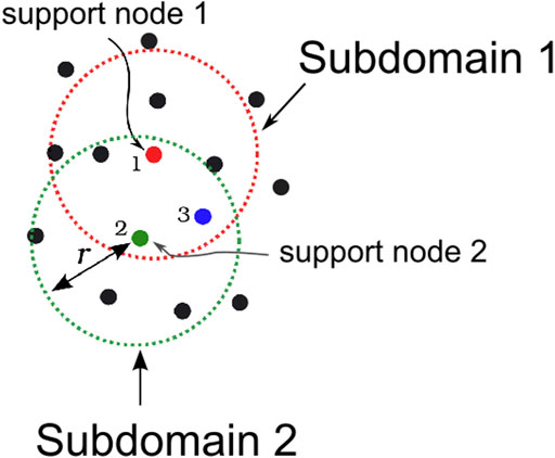
Figure 2. Illustration of meshfree subdomains. A subdomain for a point (“node”) contains a certain number of points within the chosen distance $r$ from the point. Here, subdomain 1 contains 7 meshfree points (with the support node 1 as the center), and subdomain 2 also contains 7 meshfree points.

Using the above meshfree interpolant, any differential operator $\mathbf{D}$ (e.g., ${\nabla }^2$ in Eq. 10) can be discretized over the meshfree subdomains in the form of a linear combination of $n$ local function values, a process that is similar to the traditional mesh-based finite difference approximation but in a more general treatment: $\mathbf{D}f{|}_{{\mathbf{r}}_i}\approx {\sum }_{k=1}^n{b}_k{f}_k$. In RBF-FDs, the discretization of the operator $\mathbf{D}$ is multi-dimensional, while in the classical mesh-based finite differences the discretization of $\mathbf{D}$ is restricted to be directional approximation (i.e., only 1-D). The weights, $b_k$, are then obtained by solving the following $n\times n$ local linear system

$\left(\begin{array}{cccc}\hfill R\left(\Vert {\mathbf{r}}_1-{\mathbf{r}}_1\Vert \right)\hfill & \hfill R\left(\Vert {\mathbf{r}}_1-{\mathbf{r}}_2\Vert \right)\hfill & \hfill \cdots \hfill & \hfill R\left(\Vert {\mathbf{r}}_1-{\mathbf{r}}_n\Vert \right)\hfill \\ \hfill R\left(\Vert {\mathbf{r}}_2-{\mathbf{r}}_1\Vert \right)\hfill & \hfill R\left(\Vert {\mathbf{r}}_2-{\mathbf{r}}_2\Vert \right)\hfill & \hfill \cdots \hfill & \hfill R\left(\Vert {\mathbf{r}}_2-{\mathbf{r}}_n\Vert \right)\hfill \\ \hfill ⋮\hfill & \hfill ⋮\hfill & \hfill \ddots \hfill & \hfill ⋮\hfill \\ \hfill R\left(\Vert {\mathbf{r}}_n-{\mathbf{r}}_1\Vert \right)\hfill & \hfill R\left(\Vert {\mathbf{r}}_n-{\mathbf{r}}_2\Vert \right)\hfill & \hfill \cdots \hfill & \hfill R\left(\Vert {\mathbf{r}}_n-{\mathbf{r}}_n\Vert \right)\hfill \end{array}\right)\left(\begin{array}{c}\hfill b_1\hfill \\ \hfill b_2\hfill \\ \hfill ⋮\hfill \\ \hfill b_n\hfill \end{array}\right)=\left(\begin{array}{c}\hfill \mathbf{D}{R}_1\left(\mathbf{r}\right){|}_{{\mathbf{r}}_i}\hfill \\ \hfill \mathbf{D}{R}_2\left(\mathbf{r}\right){|}_{{\mathbf{r}}_i}\hfill \\ \hfill ⋮\hfill \\ \hfill \mathbf{D}{R}_n\left(\mathbf{r}\right){|}_{{\mathbf{r}}_i}\hfill \end{array}\right),(17)$

and form as the nonzeros in the corresponding rows of the coefficient matrix $\mathbf{A}$ in the resultant $N\times N$ global linear system $\mathbf{A}\mathbf{x}=\mathbf{h}$ ($N$ is the total number of points). Here, $\mathbf{D}{R}_1(\mathbf{r}){|}_{{\mathbf{r}}_i}$ denotes the value of $\mathbf{D}{R}_1(\mathbf{r})$ at the location ${\mathbf{r}}_i$ and can be readily calculated using the chain rules of the derivatives for the chosen RBF. $\mathbf{x}$ is the vector of the unknown function values at the degrees of freedom (i.e., meshfree points in the RBF-FD). The proof of Eq. 17 is thoroughly presented in Long and Farquharson (2019b). The right-hand-side vector $\mathbf{h}$ is formed from proper boundary conditions and the discretizations of EM source terms. Note that only Eq. 17 needs to be solved in transforming the differential equations (Eq. 10 to Eq. 13) into linear systems of equations. The well-known numerical analysis package LAPACK subroutines were used to numerically solve Eq. 17. In this study, all meshfree points are unstrutured and the size of meshfree subdomains is fixed as $n=30$ (the number of points in a meshfree subdomain) and the selection of the closest $n=30$ points for each subdomain is carried out using a kd-tree point selection method which is the same as in Long and Farquharson (2019b). The fixed number of points in subdomains means that the relative distances among the $n$ points in a meshfree subdomain can be smaller (e.g., near CSEM sources) when high numerical accuracies are needed.

3 Numerical results

In this section, the modellings of different EM data using the meshfree method are demonstrated. The global linear system from discretizing the $\mathbf{A}$-$\varphi$ potential function equations is asymmetric, complex-valued and can be solved using either iterative solvers or direct solvers. In this study, all global linear systems are solved using the MUMPS direct solver (Amestoy et al., 2001, version 5.3.3).

3.1 Magnetotelluric data

The magnetotelluric (MT) conductivity model for the demonstration of the meshfree modelling is the Dublin Test Model 2 (DTM2, Miensopust et al., 2013) in which a hemispherical conductor is buried at the top of the subsurface (Figure 3). The hemispherical conductor has the resistivity of 10 $\mathrm{\Omega }$m and the background earth’s resistivity is 300 $\mathrm{\Omega }$m. The radius of the hemisphere is $R=5$ km. Because of the perfect symmetry of the conductivity structure, there exists analytical solutions of MT responses at the galvanic limit (i.e., zero-frequency limit). For the same reason, the observed MT responses will be symmetric. These features of this model make it a good example for the comparison of different numerical modelling algorithms (Miensopust et al., 2013). However, also due to the spherical surface geometry of the conductor, mesh-based modelling techniques, particularly those relying on tensor-grid or rectilinear meshes, will face challenges in accurately representing the geometry, and therefore in studying the effects of shallow inhomogeneities of the conductivity distribution on the MT data at sites near the edge of the conductor.

Figure 3

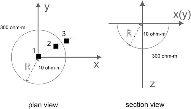
Figure 3. Schematic illustration of the Dublin Test Model 2 (DTM2). Three MT sites at the surface are marked with black squares (at $R=$ 0, 4,500 m, 5,100 m from the origin, respectively) in the plan view (left). The radius of the hemisphere conductor is $R=5000$ m.

In MT data modellings, the EM source terms in Eqs 10–13, i.e., $\mathbf{J}$ and its divergence, vanish as the actual EM sources are far away from the surface of the Earth (Long and Farquharson, 2019b). In this model, the boundary conductivity distribution is that of the uniform subsurface and 1-D boundary conditions were used to compute boundary values (see details in Long and Farquharson, 2019b). The EM responses in the MT scenario are typically represented using apparent resistivity and phase data which are calculated from the electric and magnetic fields at the measurement locations. Although the previous study using the RBF-FD method (Long and Farquharson, 2019b) has demonstrated the effectiveness of the modelling capability, particularly how the discontinuous electric field can be correctly modelled using the developed RBF-FD method here, it does not demonstrate the flexible meshfree discretization of highly irregular surface geometries as we see in the DTM2 here. The unstructured point discretization with local refinements for this model is shown in Figure 4. The total number of points in the discretization is $N=\mathrm{165,940}$ for a computational domain of $\{(x,y,z)|-30\text{km}\le x,y\le 30\text{km},-50\text{km}\le z\le 10\text{km}\}$.

Figure 4

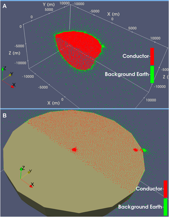
Figure 4. Perspective 3-D views of the meshfree point discretization of the Dublin Test Model 2 (DTM2). In Panel (A): unstructured points inside the conductor. In Panel (B): 3 MT sites at the surface (at $R=$ 0, 4,500 m, 5,100 m from the origin, respectively) are shown with dense points due to local refinements, and the 3-D hemisphere conductor in the original model is represented by a multi-facet polyhedron.

Three MT sites (Figure 3) are designed here to examine the modelling accuracy of the meshfree method. Site 1 is at the origin of the coordinate system and at the center of the hemisphere conductor. Site 2 ($R=4500$ m; $x=y=3182$ m) is 500 m away from the edge of the hemisphere and is inside the hemisphere (same as Site 10 in Miensopust et al. (2013)). Site 3 ($R=5100$ m; $x=y=3606$ m) is 100 m away from the edge of and outside the hemisphere (same as Site 18 in Miensopust et al. (2013)). MT responses at Site 2 and 3 are expected to be significantly affected by the irregular shape of the hemisphere for long periods. Same as Miensopust et al. (2013), the frequency range of $10^{-4}$ Hz to 100 Hz (periods from 0.01 s to 10,000 s) were used for the examination. The calculated MT responses at the three sites using the meshfree RBF-FD method were compared with other independent solutions (all using mesh-based modelling methods) that are documented from Miensopust et al. (2013) and are shown in Figures 5–7 for the three sites. At each site, the apparent resistivity and phase data for the four components of the impedance tensor (i.e., $Z_{XX}$, $Z_{XY}$, $Z_{YX}$ and $Z_{YY}$) are plotted from top to bottom.

Figure 5

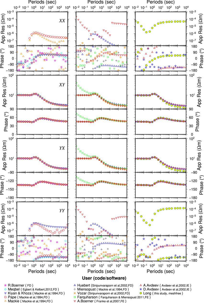
Figure 5. Comparison of the meshfree solution and other solutions for the Site-1 (origin) MT responses for DTM2. From top to bottom are XX, XY, YX, and YY components of the impedance tensor. Different users or runners of the used modelling codes are shown in the legend with algorithm acronyms as FD (finite difference), FE (finite element) and, IE (integral equation).

Figure 6

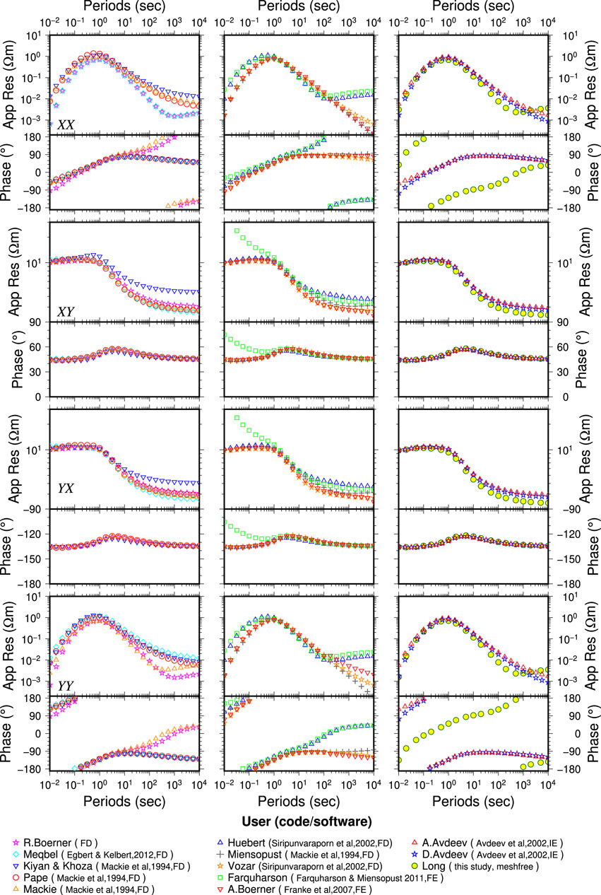
Figure 6. Comparison of the meshfree solution and other solutions for the Site-2 ($R=4500$ m) MT responses for DTM2. From top to bottom are XX, XY, YX, and YY components of the impedance tensor. Different users or runners of the used modelling codes are shown in the legend with algorithm acronyms as FD (finite difference), FE (finite element) and, IE (integral equation).

Figure 7

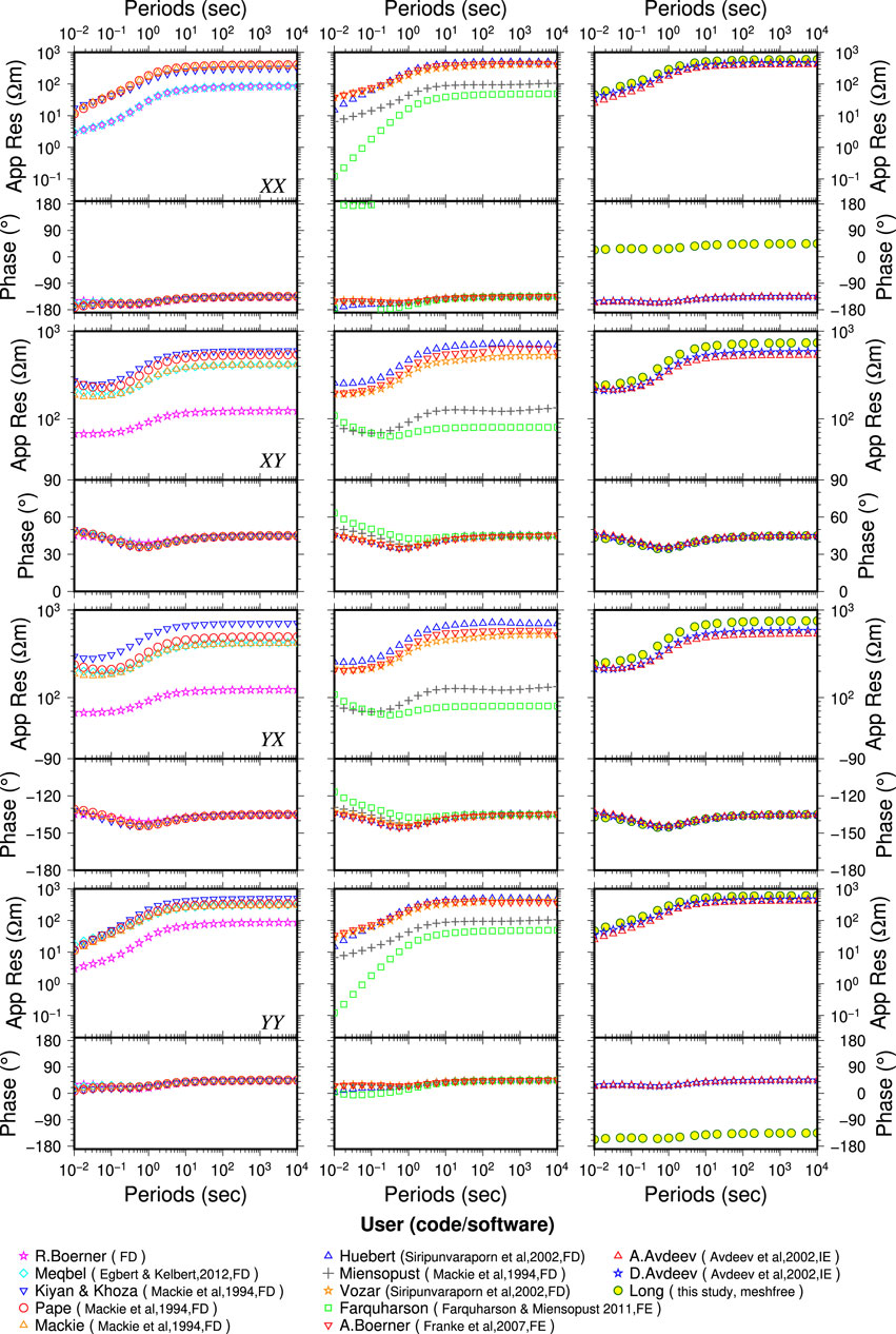
Figure 7. Comparison of the meshfree solution and other solutions for the Site-3 ($R=5100$ m) MT responses for DTM2. From top to bottom are XX, XY, YX, and YY components of the impedance tensor. Different users or runners of the used modelling codes are shown in the legend with algorithm acronyms as FD (finite difference), FE (finite element) and, IE (integral equation).

At Site 1 (Figure 5), which is at the origin of the model, the theoretical apparent resistivity of the MT responses for $Z_{XX}$ and $Z_{YY}$ are zero, which explains the extremely small and random numerical values of the apparent resistivity and phase data observed for all numerical solutions. For the off-diagonal components $Z_{XY}$ and $Z_{YX}$, almost all numerical solutions agree with each other. At Site 2 (Figure 6) and Site 3 (Figure 7), all four components of the impedance tensor will be non-zero due to the edge effect of the conductor. For the phase data in the $Z_{XX}$ and $Z_{YY}$ components at these two sites, the meshfree solution appears to deviate from other solutions; this is because of the difference in the Coordinate systems being used and the phase angle calculation methods.¹ The meshfree numerical solutions are validated by the following two observations: the symmetry in the solution (MT responses for $Z_{XX}$ and $Z_{YY}$ are the same, so are the $Z_{XY}$ and $Z_{YX}$) and the good agreement with the majority of other independent solutions. Note that among those independent solutions, a few solutions (e.g., Kiyan and Khoza) have a clear deviation from the main MT response curves in long periods (after 10 s for Site 2) due to insufficient mesh discretizations around the edge of the hemisphere conductor.

3.2 Frequency-domain controlled-source EM data

To compute the controlled-source EM (CSEM) responses, the external source terms in Eqs 10–13 ($\mathbf{J}$ and its divergence) will be non-zero at the locations of the source. Here, in the context of the meshfree RBF-FD method, the source handling method of Long and Farquharson (2019a) is used. As shown in Figure 8, any CSEM source wire is initially represented by meshfree points in space with proper distances and regularity of distribution among them. For each point representing the source wire, a local unstructured mesh is contructed by connecting the points found in the subdomain of the point. Then a finite element-like weak-form treatment (e.g., Badea et al., 2001; Jin, 2014) is used to discretize the equations at the source point in which the electrical current of the wire will be coincident with the edges of the local mesh which is of tetrahedral type in this study. The number of nodes in this local mesh is very small $(\le =n=30)$ and the mesh connectivity is generated automatically using common mesh generation software (e.g., Tetgen and Gmsh). For grounded wires, the divergence of the current density is only non-zero at the beginning and the ending source points.

Figure 8

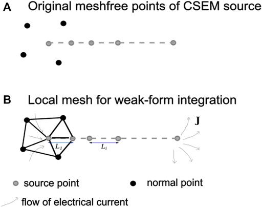
Figure 8. Schematic illustration of meshfree point representation of CSEM source wires. Panel (A): the grounded wire is represented by 5 special points designated as source points. Panel (B): for each source point, a local unstructured mesh is formed using the point (left-most source point here) and its neighbouring points.

The above method is capable of treating an arbitrarily shaped controlled source (grounded wires or current loops) in the point discretization of an Earth model. Because of this capability, the total-field approach of modelling the EM data, as described in Eqs 10–13 in the case of potential functions, is being used here and will provide more flexibility in handling complex topography and surface geometries. Under the total-field approach, the boundary values of the EM field on the computational domain is zero.

3.2.1 Half-space model

The first CSEM test model is that of a uniform subsurface with an electric dipole source at the Earth’s surface (Figure 9). Although the model is relatively ideal, analytical solutions exist for the EM fields at the surface which allows for a first-step examination of the accuracy of the developed RBF-FD meshfree method for CSEM data modellings. An $x$-directed electric dipole, for example, will have the current density ${\mathbf{J}}_s$ as (Ward and Hohmann, 1988)

${\mathbf{J}}_s=I_0\left[\mathcal{H}\left(x_1\right)-\mathcal{H}\left(x_2\right)\right]\delta \left(y-y_0\right)\delta \left(z-z_0\right)\widehat{\mathbf{x}},(18)$

where $I_0$ is the current intensity, $\mathcal{H}(x)$ is Heaviside function, $(x_1,y_0,z_0)$ and $(x_2,y_0,z_0)$ are the two ends of the grounded wire, and $\delta$ is the Dirac delta function. The closed-form, analytical formula (eq. 4.159 in Ward and Hohmann, 1988) for computing the inline electric field due to the above CSEM transmitter (Eq. 18) for any measurement locations at the surface of the subsurface (i.e., at $z=0$) is:

$E_x\left(x,y\right)=\frac{I_0\mathit{\text{ds}}}{2\pi \sigma {\rho }^3}\left[1+\left(ik\rho +1\right)e^{-ik\rho }-\frac{3y^2}{{\rho }^2}\right],(19)$

where $\rho =\sqrt{x^2+y^2}$, $k=-i\omega \mu \sigma$ is the wavenumber with $\sigma$ as the conductivity of the subsurface. In the case of dipole sources where the length of the grounded wire approaches infinitesimally small in relative to the distance from the dipole to measurement locations, $ds=1$in Eq. 19.

Figure 9

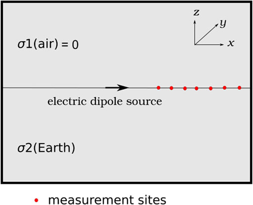
Figure 9. A half-space conductivity model with the horizontal electric dipole source (black arrow) at the top of the subsurface. Adapted from Long and Farquharson (2019a).

The current density of the electric dipole source is set to be 1 A. For the meshfree solution, a set of unstructured points with local refinements around the dipole source was used. The actual CSEM source in the meshfree modelling is 1 m in length along the $x$ direction and is represented by six points with the equal spacing of 0.2 m from $x=-0.5$ m to $x=0.5$ m. Four frequencies at $f=\mathrm{3,0.3},10^{-4}$ and $10^{-8}$ Hz were used for the accuracy examination. The uniform Earth’s subsurface has the conductivity of 0.02 S/m. With this conductivity value, the very low frequency of $10^{-8}$ Hz will approach the direct current limit and the electric field responses will approach those of a direct current resistivity survey. The total number of the points for the model discretization is 81,951 which are distributed within the computational domain $\{(x,y,z)|-40\text{km}\le x,y,z\le 40\text{km}\}$ where the dipole is located at the center. The computed $E_x$ responses at the surface $(y=z=0)$ are shown in Figure 10. As evident from the comparison, the two solutions have an excellent agreement with each other, demonstrating the computational accuracy of the meshfree method. At the highest frequency $f=3$ Hz (Figure 10A), the imaginary $E_x$ from the meshfree numerical solution starts to deviate from the theoretical solution when $\Vert x\Vert \ge 7$ km. This deviation is due to the decreased point density after the distance. At lower frequencies, such deviation vanishes due to less rapid changes of the EM field at the same locations. In addition, when the frequency approaches the direct current limit (Figure 10C,D), the frequency-domain $E_x$ response has the real part almost unchanged but the imaginary part continuously decreased until zero; that is, $E_x$ response is approaching the direct current resistivity response, which is another evidence of the correct modelling of the CSEM responses.

Figure 10

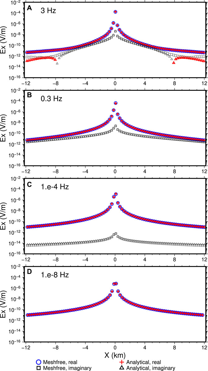
Figure 10. Comparison between the meshfree and the analytical solutions. From (A–D), each panel shows the real and imaginary parts of $E_x$ of the two solutions at a different frequency. All real part values are positive. The imaginary part values are all negative values except for bold, colored symbols (as the imaginary analytical solution at $f=3$ Hz shows). In panel (D), the imaginary $E_x$ values are outside the range and are not shown.

3.2.2 Ovoid mineral deposit model

The second CSEM test example is from the volcanic massive sulphide mineral deposit (termed as Ovoid deposit here) from Voisey’s Bay, Labrador, Canada, which has been under extensive studies for both geology and geophysical data modelling studies (e.g., Jahandari and Farquharson, 2014; Li J. et al., 2017; Long and Farquharson, 2019c; Kara and Farquharson, 2023). The Ovoid deposit is a highly conductive iron-dominant deposit with complex surface geometry which serves as a perfect testing example for geophysical data modelling software. To test the meshfree modelling method developed here, the real topography of the Earth’s surface (also see Jahandari and Farquharson, 2014; Kara and Farquharson, 2023) has been used here. The nearest point of the deposit to the surface is about 70 m below the uneven surface (see Figure 11). Following Kara and Farquharson (2023), a grounded wire of 400 m long with a current density of 1 A along the easting direction (Figure 11A,B) is used as the source for a ground EM survey. The offset of the wire source is roughly 600 m away from the central part of the deposit. There are 143 measurement sites at the surface designed as receiver locations which are distributed evenly along 11 South-to-North profiles (Figure 11C). The profile spacing is 100 m. The site spacing along each profile is approximately 50 m. The highly conductive deposit is assumed to have a uniform conductivity of 1 S/m here and the relatively resistive background earth is assigned the conductivity of 0.001 S/m. Both conductivity values are taken from the previous test model of Kara and Farquharson (2023) for facilitating a direct comparison of the meshfree modelling results with theirs.

Figure 11

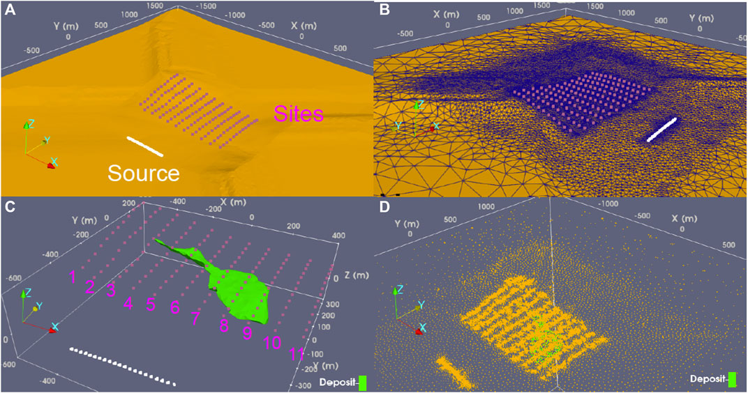
Figure 11. 3-D views of the CSEM configuration of the Ovoid deposit model. Panels (A) and (B): two different views of the grounded wire source (white dots) and the CSEM measurement sites (purple dots) overlaying the Earth’s surface with topography. Panel (C): the geometry of the Ovoid mineral deposit in the subsurface and the 11 profiles of measurement sites numbered from 1 ($x=-600$ m) to 11 ($x=400$ m) from west to east. Panel (D): meshfree point discretization of the subsurface when viewed from the air, with the CSEM source and site locations locally refined.

For the model discretization, the meshfree points used here are also directly taken from the point distribution from the tetrahedral mesh used by Kara and Farquharson (2023) which are visualized in Figure 11D. In their modelling, they have used a vector finite element method for computing the CSEM responses. For both finite element methods and meshfree methods, the local refinements around the transmitter and the receiver locations are necessary to improve the numerical modelling accuracy. The 400-m long grounded wire is represented in the meshfree method using 80 points located at the topographic surface with in average 5 m of distance apart from each other (see Figure 8). The total number of points for this discretization is 44,230 within the computational domain of $\{(x,y,z)|-20\text{km}\le x,y,z\le 20\text{km}\}$. For long grounded wire sources, the inline electric field and vertical magnetic field components are often the main measurements. The computed $E_x$ and $H_z$ responses using the meshfree method are compared with the finite element results of Kara and Farquharson (2023) which are shown in Figures 12–14 at the measurement site profiles $x=\mathrm{400,0},-200$ m (also see Figure 11C), respectively, for the frequency of 500 Hz. It is seen that the two independent solutions, calculated using the same model discretization (i.e., meshfree points and tetrahedral mesh), have a very good agreement with each other for all sites (see supplemental materials for the comparison for the remaining profiles). The strong EM induction caused by the deposit is well reflected at the sites that are more closely above the deposit (see the profiles $x=-200$ m and $x=0$ m). The higher frequency (i.e., $f=1500$ Hz) responses for the profile $x=-200$ (Profile 5) is also shown in Figure 15. Comparing Figure 15 with Figure 14, it is seen that at the higher frequency, the EM responses, particularly $H_z$ responses, attenuate faster in space.

Figure 12

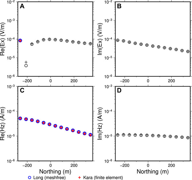
Figure 12. Computed $E_x$ and $H_z$ components of the CSEM responses at $f=500$ Hz over the Ovoid model at the site profile $x=400$ m (Profile 11 in Figure 11 (c)). Panels (A) and (B): real and imaginary parts of $E_x$, respectively. Panels (C) and (D): real and imaginary parts of $H_z$, respectively. Bold, colored symbols indicate positive values; thin, black symbols represent negative values.

Figure 13

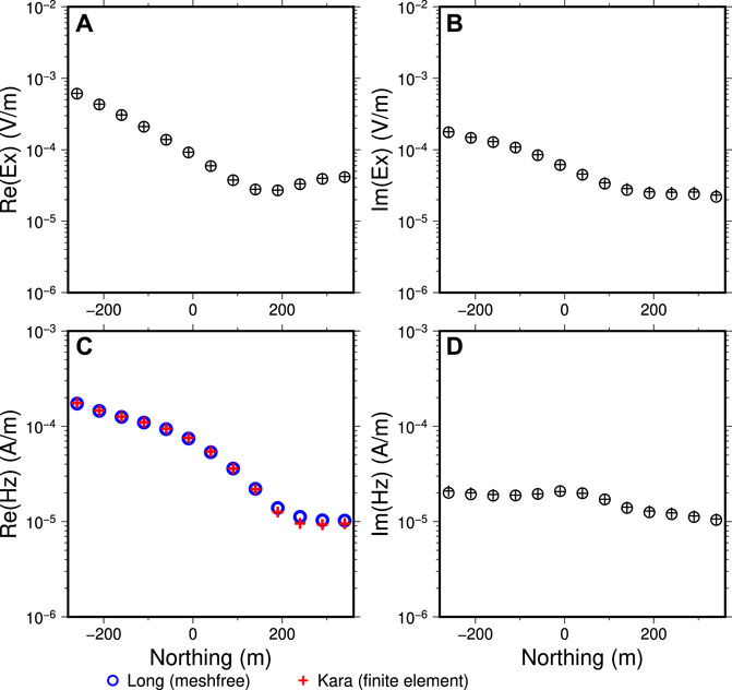
Figure 13. Computed $E_x$ and $H_z$ components of the CSEM responses at $f=500$ Hz over the Ovoid model at the site profile $x=0$ m (Profile 7 in Figure 11C). Panels (A) and (B): real and imaginary parts of $E_x$, respectively. Panels (C) and (D): real and imaginary parts of $H_z$, respectively. Bold, colored symbols indicate positive values; thin, black symbols represent negative values.

Figure 14

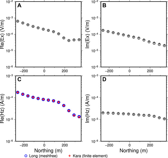
Figure 14. Computed $E_x$ and $H_z$ components of the CSEM responses at $f=500$ Hz over the Ovoid model at the site profile $x=-200$ m (Profile 5 in Figure 11C). Panels (A) and (B): real and imaginary parts of $E_x$, respectively. Panels (C) and (D): real and imaginary parts of $H_z$, respectively. Bold, colored symbols indicate positive values; thin, black symbols represent negative values.

Figure 15

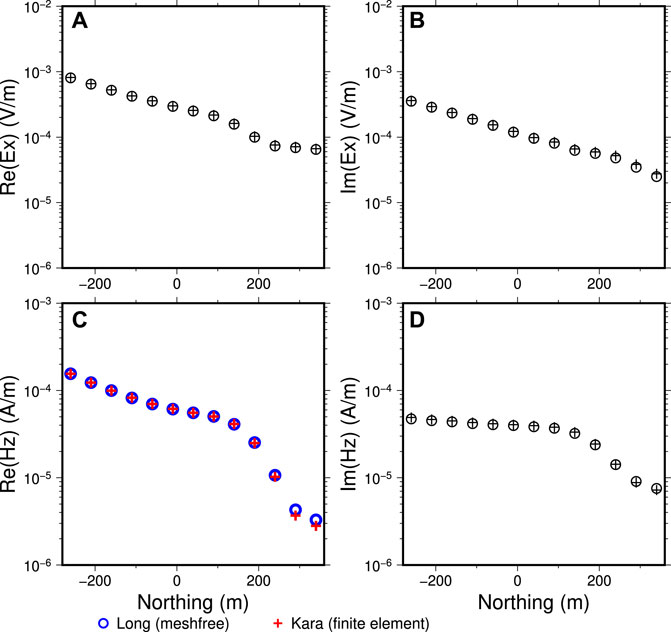
Figure 15. Same CSEM responses as in Figure 14 but at $f=1500$ Hz. Panels (A,B): real and imaginary parts of Ex, respectively. Panels (C,D): real and imaginary parts of Hz, respectively. Bold, colored symbols indicate positive values; thin, black symbols represent negative values.

4 Discussions

Direct current resistivity (DCR) survey methods are also frequently used for mineral resource exploration. Although I have not directly shown the modelling capability of the meshfree method for DCR data modelling, the first CSEM modelling example (in the case of $freq\to 0$) is essentially a simple demonstration of how the developed meshfree modelling approach can be directly applied to compute DCR data for a general conductivity model. When the frequency is zero, the potential function equations described in Eqs 10–13 will be reduced to the exact potential function equation (i.e., Poisson’s equation for $\varphi$) used for DCR data computation.

For model discretization, the unstructured meshfree points were generated using a combination of existing open-source software tools (including Tetgen and Paraview). The geophysical community is likely to continue to benefit from research in other fields. In the situation of dedicated software development for meshfree point generation, there have been significant research and development in the past decade (Fornberg and Flyer, 2015). It is anticipated that, like the history of the classical finite element methods, more open-source point generation tools will be available once the meshfree methods along with their capability of incorporating complex geometries become more widely known.

5 Conclusion

Earth models in the context of mineral resource exploration using geophysical survey methods often have rather complex surface geometries. It is important that the numerical forward modelling of geophysical EM data for such models is capable of efficiently handling these geometries. A meshfree modelling method that uses only unconnected points, instead of the traditional pixel cell-based meshes, to represent geometries has been developed and presented here. The $\mathbf{A}$-$\varphi$ potential equations instead of the Helmholtz equation for the electric field are used for the continuity property of the potential functions. The meshfree method supports both uniform and non-uniform, unstructured point distributions with the latter being of particularly advantageous in discretizing Earth models with complex geometries with a minimal amount of points.

The modelling accuracy and the capability of handling highly irregular surface geometries of the method are demonstrated using three EM modelling examples. The first example is a magnetotelluric model in which the magnetotelluric impedance responses of a hemisphere-shaped near-surface conductor were modelled. The second example is an idealized half-space conductivity model excited with a grounded electric dipole source for which closed-form analytical solutions exist. The third example, which is also a controlled-source example, is the real-life highly conductive Ovoid mineral deposit model in which the realistic surface geometry of the deposit and the topography were used. The EM transmitter for this example is a 400 m long grounded wire. Through these examples, the feasibility of easily representing irregular surface geometries of the Earth models is clearly demonstrated. The point discretizations are considered to be more advantageous over traditional mesh discretizations for complex Earth models as they are easier to generate and manipulate. For all examples, the modelling accuracies of the meshfree method are verified using other independent numerical solutions or analytical solutions.

The demonstrated meshfree modelling method is also applicable to other geophysical data modellings in which numerical solutions and complex geometries of the model are important. The developed meshfree method for geophysical EM data modellings is shown to be effective for both natural-source magnetotelluric surveys and controlled-source EM surveys. For the magnetotelluric example, the meshing of the spherical surface geometry is a non-trivial task, especially for numerical methods that are restricted to the use of rectilinear meshes, as evident from the large differences of modelled magnetotelluric responses among some independent solutions (Miensopust et al., 2013). The representation of such geometry is however quite straightforward and easy in the meshfree point discretization.

Data availability statement

The raw data supporting the conclusions of this article will be made available by the authors, without undue reservation.

Author contributions

JL: Conceptualization, Data curation, Investigation, Methodology, Software, Writing–original draft, Writing–review and editing.

Funding

The author(s) declare that no financial support was received for the research, authorship, and/or publication of this article.

Acknowledgments

Kara and Farquharson are thanked for graciously providing the mesh data to build the Ovoid deposit model discretization and for sharing their finite element solutions to compare with in this study.

Conflict of interest

The author declares that the research was conducted in the absence of any commercial or financial relationships that could be construed as a potential conflict of interest.

Publisher’s note

All claims expressed in this article are solely those of the authors and do not necessarily represent those of their affiliated organizations, or those of the publisher, the editors and the reviewers. Any product that may be evaluated in this article, or claim that may be made by its manufacturer, is not guaranteed or endorsed by the publisher.

Footnotes

¹The solutions provided from Miensopust et al. (2013) only have the computed phase angles, rather than the impedance values themselves

References

Amestoy, P., Duff, I. S., Koster, J., and L’Excellent, J.-Y. (2001). A fully asynchronous multifrontal solver using distributed dynamic scheduling. SIAM J. Matrix Analysis Appl. 23, 15–41. doi:10.1137/s0895479899358194

CrossRef Full Text | Google Scholar

Ansari, S., and Farquharson, C. G. (2014). 3D finite-element forward modeling of electromagnetic data using vector and scalar potentials and unstructured grids. Geophysics 79, E149–E165. doi:10.1190/geo2013-0172.1

CrossRef Full Text | Google Scholar

Badea, E. a., Everett, M. E., Newman, G. a., and Biro, O. (2001). Finite-element analysis of controlled-source electromagnetic induction using Coulomb-gauged potentials. Geophysics 66, 786–799. doi:10.1190/1.1444968

CrossRef Full Text | Google Scholar

Buhmann, M. D. (2003). Radial basis functions. Cambridge: Cambridge University Press. doi:10.1017/CBO9780511543241

CrossRef Full Text | Google Scholar

Chen, C., Kruglyakov, M., and Kuvshinov, A. (2021). Advanced three-dimensional electromagnetic modelling using a nested integral equation approach. Geophys. J. Int. 226, 114–130. doi:10.1093/gji/ggab072

CrossRef Full Text | Google Scholar

Chen, J.-S., Hillman, M., and Chi, S.-W. (2017). Meshfree methods: progress made after 20 years. J. Eng. Mech. 143, 04017001. doi:10.1061/(asce)em.1943-7889.0001176

CrossRef Full Text | Google Scholar

Coggon, J. H. (1971). Electromagnetic and electrical modeling by the finite element method. Geophysics 36, 132–155. doi:10.1190/1.1440151

CrossRef Full Text | Google Scholar

Du, Q., Gunzburger, M., and Ju, L. (2002). Meshfree, probabilistic determination of point sets and support regions for meshless computing. Comput. methods Appl. Mech. Eng. 191, 1349–1366. doi:10.1016/s0045-7825(01)00327-9

CrossRef Full Text | Google Scholar

Du, Q., Wang, D., and Zhu, L. (2009). On mesh geometry and stiffness matrix conditioning for general finite element spaces. SIAM J. Numer. Analysis 47, 1421–1444. doi:10.1137/080718486

CrossRef Full Text | Google Scholar

Dyck, A. V., and West, G. F. (1984). The role of simple computer models in interpretations of wide-band, drill-hole electromagnetic surveys in mineral exploration. Geophysics 49, 957–980. doi:10.1190/1.1441741

CrossRef Full Text | Google Scholar

Fabri, A., Giezeman, G.-J., Kettner, L., Schirra, S., and Schönherr, S. (2000). On the design of CGAL a computational geometry algorithms library. Softw. Pract. Exp. 30, 1167–1202. doi:10.1002/1097-024x(200009)30:11<1167::aid-spe337>3.0.co;2-b

CrossRef Full Text | Google Scholar

Farquharson, C. G., and Craven, J. A. (2009). Three-dimensional inversion of magnetotelluric data for mineral exploration: an example from the McArthur River uranium deposit, Saskatchewan, Canada. J. Appl. Geophys. 68, 450–458. doi:10.1016/j.jappgeo.2008.02.002

CrossRef Full Text | Google Scholar

Farquharson, C. G., and Oldenburg, D. W. (2002). An integral equation solution to the geophysical electromagnetic forward-modelling problem. Methods Geochem. Geophys. (Elsevier) 35, 3–19. doi:10.1016/S0076-6895(02)80083-X

CrossRef Full Text | Google Scholar

Fasshauer, G. E. (2007). Meshfree approximation methods with matlab, vol. 6 of Interdiscip. Math. Sci. World Sci. doi:10.1142/6437

CrossRef Full Text | Google Scholar

Fornberg, B., and Flyer, N. (2015). Fast generation of 2-D node distributions for mesh-free PDE discretizations. Comput. Math. Appl. 69, 531–544. doi:10.1016/j.camwa.2015.01.009

CrossRef Full Text | Google Scholar

Gehrmann, R., North, L. J., Graber, S., Szitkar, F., Petersen, S., Minshull, T., et al. (2019). Marine mineral exploration with controlled source electromagnetics at the TAG hydrothermal field, 26°N mid-atlantic ridge. Geophys. Res. Lett. 46, 5808–5816. doi:10.1029/2019gl082928

CrossRef Full Text | Google Scholar

Günther, T., Rücker, C., and Spitzer, K. (2006). Three-dimensional modelling and inversion of DC resistivity data incorporating topography-II. Inversion. Geophys. J. Int. 166, 506–517. doi:10.1111/j.1365-246x.2006.03011.x

CrossRef Full Text | Google Scholar

Han, B., Li, Y., and Li, G. (2018). 3D forward modeling of magnetotelluric fields in general anisotropic media and its numerical implementation in Julia. Geophysics 83, F29–F40. doi:10.1190/geo2017-0515.1

CrossRef Full Text | Google Scholar

Hohmann, G. W. (1975). Three-dimensional induced polarization and electromagnetic modeling. Geophysics 40, 309–324. doi:10.1190/1.1440527

CrossRef Full Text | Google Scholar

Jahandari, H., Ansari, S., and Farquharson, C. G. (2017). Comparison between staggered grid finite–volume and edge–based finite–element modelling of geophysical electromagnetic data on unstructured grids. J. Appl. Geophys. 138, 185–197. doi:10.1016/j.jappgeo.2017.01.016

CrossRef Full Text | Google Scholar

Jahandari, H., Bihlo, A., and Donzelli, F. (2021). Forward modelling of gravity data on unstructured grids using an adaptive mimetic finite-difference method. J. Appl. Geophys. 190, 104340. doi:10.1016/j.jappgeo.2021.104340

CrossRef Full Text | Google Scholar

Jahandari, H., and Farquharson, C. G. (2014). A finite-volume solution to the geophysical electromagnetic forward problem using unstructured grids. Geophysics 79, E287–E302. doi:10.1190/geo2013-0312.1

CrossRef Full Text | Google Scholar

Jia, X., and Hu, T. (2006). Element-free precise integration method and its applications in seismic modelling and imaging. Geophys. J. Int. 166, 349–372. doi:10.1111/j.1365-246X.2006.03024.x

CrossRef Full Text | Google Scholar

Jin, J.-M. (2014). The finite element method in electromagnetics. 3 edn. USA: John Wiley & Sons.

Google Scholar

Jones, A. G. (2023). Mining for net zero: the impossible task. Lead. Edge 42, 266–276. doi:10.1190/tle42040266.1

CrossRef Full Text | Google Scholar

Jones, F. W., and Pascoe, L. J. (1972). The perturbation of alternating geomagnetic fields by three-dimensional conductivity inhomogeneities. Geophys. J. Int. 27, 479–485. doi:10.1111/j.1365-246X.1972.tb06103.x

CrossRef Full Text | Google Scholar

Kara, K. B., and Farquharson, C. G. (2023). 3D minimum-structure inversion of controlled-source EM data using unstructured grids. J. Appl. Geophys. 209, 104897. doi:10.1016/j.jappgeo.2022.104897

CrossRef Full Text | Google Scholar

Key, K., and Ovall, J. (2011). A parallel goal-oriented adaptive finite element method for 2.5-D electromagnetic modelling. Geophys. J. Int. 186, 137–154. doi:10.1111/j.1365-246x.2011.05025.x

CrossRef Full Text | Google Scholar

Lelièvre, P., Carter-McAuslan, A., Farquharson, C., and Hurich, C. (2012). Unified geophysical and geological 3D Earth models. Lead. Edge 31, 322–328. doi:10.1190/1.3694900

CrossRef Full Text | Google Scholar

Li, B., Liu, Y., Sen, M. K., and Ren, Z. (2017a). Time-space-domain mesh-free finite difference based on least squares for 2D acoustic-wave modeling. Geophysics 82, T143–T157. doi:10.1190/geo2016-0464.1

CrossRef Full Text | Google Scholar

Li, J., Farquharson, C. G., and Hu, X. (2017b). 3D vector finite-element electromagnetic forward modeling for large loop sources using a total-field algorithm and unstructured tetrahedral grids. Geophysics 82, E1–E16. doi:10.1190/geo2016-0004.1

CrossRef Full Text | Google Scholar

Liu, Z., Ren, Z., Yao, H., Tang, J., Lu, X., and Farquharson, C. (2023). A parallel adaptive finite-element approach for 3-D realistic controlled-source electromagnetic problems using hierarchical tetrahedral grids. Geophys. J. Int. 232, 1866–1885. doi:10.1093/gji/ggac419

CrossRef Full Text | Google Scholar

Long, J., and Farquharson, C. G. (2017). “Three-dimensional controlled-source EM modeling with radial basis function-generated finite differences: a meshless approach,” in SEG technical program expanded abstracts 2017 (China: Society of Exploration Geophysicists), 1209–1213.

CrossRef Full Text | Google Scholar

Long, J., and Farquharson, C. G. (2019a). “Meshfree modelling of 3-D controlled-source EM data: a new method to treat the singular source terms,” in SEG technical program expanded abstracts 2019 (China: Society of Exploration Geophysicists), 1050–1054.

CrossRef Full Text | Google Scholar

Long, J., and Farquharson, C. G. (2019b). On the forward modelling of three-dimensional magnetotelluric data using a radial-basis-function-based mesh-free method. Geophys. J. Int. 219, 394–416. doi:10.1093/gji/ggz306

CrossRef Full Text | Google Scholar

Long, J., and Farquharson, C. G. (2019c). Three-dimensional forward modelling of gravity data using mesh-free methods with radial basis functions and unstructured nodes. Geophys. J. Int. 217, 1577–1601. doi:10.1093/gji/ggz115

CrossRef Full Text | Google Scholar

Long, J., and Farquharson, C. G. (2020). “Meshfree modelling of 2D MT data with RBF-FD and unstructured points,” in SEG international exposition and annual meeting (SEG). China, SEG.

CrossRef Full Text | Google Scholar

Long, J., and Farquharson, C. G. (2024). Three-dimensional controlled-source electromagnetic data modelling with a hybrid meshfree-finite element approach. Germany: preparation.

Google Scholar

Lu, X., Farquharson, C. G., Miehé, J.-M., and Harrison, G. (2021). 3D electromagnetic modeling of graphitic faults in the Athabasca Basin using a finite-volume time-domain approach with unstructured grids. Geophysics 86, B349–B367. doi:10.1190/geo2020-0657.1

CrossRef Full Text | Google Scholar

Mackie, R. L., Madden, T. R., and Wannamaker, P. E. (1993). Three-dimensional magnetotelluric modeling using difference equations—theory and comparisons to integral equation solutions. Geophysics 58, 215–226. doi:10.1190/1.1443407

CrossRef Full Text | Google Scholar

Miensopust, M. P., Queralt, P., Jones, A. G., and modellers, D. M. (2013). Magnetotelluric 3-D inversion—a review of two successful workshops on forward and inversion code testing and comparison. Geophys. J. Int. 193, 1216–1238. doi:10.1093/gji/ggt066

CrossRef Full Text | Google Scholar

Nabighian, M. N. (1988). Electromagnetic methods in applied geophysics: voume 1, theory. Germany: Society of Exploration Geophysicists.

Google Scholar

Nalepa, M., Ansari, S., and Farquharson, C. (2016). “Finite-element simulation of 3D CSEM data on unstructured meshes: an example from the East Coast of Canada,” in SEG technical program expanded abstracts 2016 (Germany: Society of Exploration Geophysicists), 1048–1052.

CrossRef Full Text | Google Scholar

Nam, M. J., Kim, H. J., Song, Y., Lee, T. J., Son, J.-S., and Suh, J. H. (2007). 3D magnetotelluric modelling including surface topography. Geophys. Prospect. 55, 277–287. doi:10.1111/j.1365-2478.2007.00614.x

CrossRef Full Text | Google Scholar

Newman, G. A. (2014). A review of high-performance computational strategies for modeling and imaging of electromagnetic induction data. Surv. Geophys. 35, 85–100. doi:10.1007/s10712-013-9260-0

CrossRef Full Text | Google Scholar

Newman, G. A., and Alumbaugh, D. L. (1995). Frequency-domain modelling of airborne electromagnetic responses using staggered finite differences. Geophys. Prospect. 43, 1021–1042. doi:10.1111/j.1365-2478.1995.tb00294.x

CrossRef Full Text | Google Scholar

Newman, G. A., Hohmann, G. W., and Anderson, W. L. (1986). Transient electromagnetic response of a three-dimensional body in a layered earth. Geophysics 51, 1608–1627. doi:10.1190/1.1442212

CrossRef Full Text | Google Scholar

Nguyen, V. P., Rabczuk, T., Bordas, S., and Duflot, M. (2008). Meshless methods: a review and computer implementation aspects. Math. Comput. Simul. 79, 763–813. doi:10.1016/j.matcom.2008.01.003

CrossRef Full Text | Google Scholar

Oden, J. T., and Prudhomme, S. (2001). Goal-oriented error estimation and adaptivity for the finite element method. Comput. Math. Appl. 41, 735–756. doi:10.1016/s0898-1221(00)00317-5

CrossRef Full Text | Google Scholar

Pridmore, D., Hohmann, G., Ward, S., and Sill, W. (1981). An investigation of finite-element modeling for electrical and electromagnetic data in three dimensions. Geophysics 46, 1009–1024. doi:10.1190/1.1441239

CrossRef Full Text | Google Scholar

Puzyrev, V., Koldan, J., de la Puente, J., Houzeaux, G., Vazquez, M., and Cela, J. M. (2013). A parallel finite-element method for three-dimensional controlled-source electromagnetic forward modelling. Geophys. J. Int. 193, 678–693. doi:10.1093/gji/ggt027

CrossRef Full Text | Google Scholar

Rabczuk, T., and Belytschko, T. (2005). Adaptivity for structured meshfree particle methods in 2D and 3D. Int. J. Numer. Methods Eng. 63, 1559–1582. doi:10.1002/nme.1326

CrossRef Full Text | Google Scholar

Ren, Z., Kalscheuer, T., Greenhalgh, S., and Maurer, H. (2013). A goal-oriented adaptive finite-element approach for plane wave 3-D electromagnetic modelling. Geophys. J. Int. 194, 700–718. doi:10.1093/gji/ggt154

CrossRef Full Text | Google Scholar

Rochlitz, R., Skibbe, N., and Günther, T. (2019). custEM: customizable finite-element simulation of complex controlled-source electromagnetic data. Geophysics 84, F17–F33. doi:10.1190/geo2018-0208.1

CrossRef Full Text | Google Scholar

Schulz, K. J., DeYoung Jr, J. H., Seal II, R. R., and Bradley, D. C. (2017). Critical mineral resources of the United States—an introduction. Tech. Rep. U. S. Geol. Surv. doi:10.3133/pp1802A

CrossRef Full Text | Google Scholar

Schwarzbach, C., Börner, R.-U., and Spitzer, K. (2011). Three-dimensional adaptive higher order finite element simulation for geo-electromagnetics-a marine CSEM example. Geophys. J. Int. 187, 63–74. doi:10.1111/j.1365-246X.2011.05127.x

CrossRef Full Text | Google Scholar

Si, H. (2015). TetGen, a delaunay-based quality tetrahedral mesh generator. ACM Trans. Math. Softw. 41, 1–36. doi:10.1145/2629697

CrossRef Full Text | Google Scholar

Slak, J., and Kosec, G. (2019). On generation of node distributions for meshless PDE discretizations. SIAM J. Sci. Comput. 41, A3202–A3229. doi:10.1137/18m1231456

CrossRef Full Text | Google Scholar

Smith, R. (2014). Electromagnetic induction methods in mining geophysics from 2008 to 2012. Surv. Geophys. 35, 123–156. doi:10.1007/s10712-013-9227-1

CrossRef Full Text | Google Scholar

Spitzer, K. (2024). Electromagnetic modeling using adaptive grids–Error estimation and geometry representation. Surv. Geophys. 45, 277–314. doi:10.1007/s10712-023-09794-9

CrossRef Full Text | Google Scholar

Strangway, D., Swift Jr, C., and Holmer, R. (1973). The application of audio-frequency magnetotellurics (AMT) to mineral exploration. Geophysics 38, 1159–1175. doi:10.1190/1.1440402

CrossRef Full Text | Google Scholar

Stratton, J. A. (2007). Electromagnetic theory. USA: John Wiley & Sons.

Google Scholar

Streich, R. (2009). 3D finite-difference frequency-domain modeling of controlled-source electromagnetic data: direct solution and optimization for high accuracy. Geophysics 74, F95–F105. doi:10.1190/1.3196241

CrossRef Full Text | Google Scholar

Taflove, A., and Umashankar, K. R. (1990). The finite-difference time-domain method for numerical modeling of electromagnetic wave interactions. Electromagnetics 10, 105–126. doi:10.1080/02726349008908231

CrossRef Full Text | Google Scholar

Takekawa, J., Mikada, H., and Imamura, N. (2015). A mesh-free method with arbitrary-order accuracy for acoustic wave propagation. Comput. Geosciences 78, 15–25. doi:10.1016/j.cageo.2015.02.006

CrossRef Full Text | Google Scholar

Wait, J. R. (1960). Propagation of electromagnetic pulses in a homogeneous conducting earth. Appl. Sci. Res. Sect. B 8, 213–253. doi:10.1007/bf02920058

CrossRef Full Text | Google Scholar

Wang, T., and Hohmann, G. W. (1993). A finite-difference, time-domain solution for three-dimensional electromagnetic modeling. Geophysics 58, 797–809. doi:10.1190/1.1443465

CrossRef Full Text | Google Scholar

Ward, S. H., and Hohmann, G. W. (1988). 4. Electromagnetic theory for geophysical applications. Electromagn. Methods Appl. Geophys. 1 (4), 130–311. doi:10.1190/1.9781560802631.ch4

CrossRef Full Text | Google Scholar

Wittke, J., and Tezkan, B. (2014). Meshfree magnetotelluric modelling. Geophys. J. Int. 198, 1255–1268. doi:10.1093/gji/ggu207

CrossRef Full Text | Google Scholar

Yee, K. S. (1966). Numerical solution of initial boundary value problems involving Maxwell’s equations in isotropic media. IEEE Trans. Antennas Propag. 14, 302–307. doi:10.1109/TAP.1966.1138693

CrossRef Full Text | Google Scholar

Zeng, S., Hu, X., Li, J., Farquharson, C. G., Wood, P. C., Lu, X., et al. (2019). Effects of full transmitting-current waveforms on transient electromagnetics: insights from modeling the Albany graphite deposit. Geophysics 84, E255–E268. doi:10.1190/geo2018-0573.1

CrossRef Full Text | Google Scholar

Zhang, B., Yin, C., Ren, X., Liu, Y., and Qi, Y. (2018). Adaptive finite element for 3d time-domain airborne electromagnetic modeling based on hybrid posterior error estimation. Geophysics 83, WB71–WB79. doi:10.1190/geo2017-0544.1

CrossRef Full Text | Google Scholar

Zhdanov, M. S. (2010). Electromagnetic geophysics: notes from the past and the road ahead. Geophysics 75, 75A49–75A66. doi:10.1190/1.3483901

CrossRef Full Text | Google Scholar