 Zhang Junke
 Zhou Lei
 Wang Xinyu
 Xie Xingbing
 Mao Yurong
 Yan Liangjun
- 1College of Geophysics and Petroleum Resources, Yangtze University, Wuhan, Hubei, China
- 2Key Laboratory of Exploration Technologies for Oil and Gas Resources, Ministry of Education, Yangtze University, Wuhan, Hubei, China
- 3School of Geophysics and Geomatics, China University of Geosciences (Wuhan), Wuhan, Hubei, China
The borehole induced polarization method has been widely used in deep mineral exploration, oil and gas resource exploration, and water resource exploration because of its high efficiency and good exploration effect. At present, the related research on the cross-well induced polarization method assumes that the underground medium is isotropic, but the electrical characteristics of the actual earth medium are anisotropic. To analyze the influence of the anisotropic characteristics on the cross-well induced polarization method, in this paper, the anisotropic forward algorithm of conductivity and polarizability in different principal axis directions based on the finite element method is studied. A three-dimensional forward simulation of the cross-well induced polarization method in anisotropic media is realized. The effectiveness and correctness of the algorithm are verified by testing and comparing complex 3-D isotropic and anisotropic models. Anisotropic geological models of the horizontal plate and inclined plate are constructed to analyze the anisotropic influences of conductivity and polarizability in different principal axis directions on the cross-well induced polarization response. The results show that the emitter sources with different depths in the well have different influences on the electrical response of the plates. Anisotropic conductivity and polarizability in horizontal plates exhibit most pronounced characteristics in the x-direction, significantly influencing the apparent polarizability curves. However, when the resistivity and polarizability are both anisotropic, the change in the z-direction is the most complicated. When the plate is inclined, the amplitude of the electrical response curve decreases to a certain extent, and the position where the amplitude appears shifts to different degrees. Notably, the response curves of the y-direction anisotropy are basically consistent with the response curves of the isotropy, regardless of the anisotropy of the conductivity and polarizability or anomalous body tilts. The results of this study improve our understanding of the influence of anisotropy on cross-well induced polarization and provide theoretical support for the interpretation of cross-well induced polarization data considering anisotropy.
1 Introduction
With the development and advancement of science and technology, the demand for mineral resources such as oil and metal deposits is continuously increasing in China. Along with the progressive exploration of surface and near-surface metal deposits, the possibility of finding large or super-large metal deposits in the near surface is getting smaller, thus deep mineral exploration techniques emerged (Mi, 2019). Geophysical prospecting methods have been applied in mineral exploration for more than one hundred years and have played a vital role. Underground geophysical prospecting as an important geophysical prospecting method. It is characterized by a high signal-to-noise ratio, anti-interference and large exploration depth. And it plays an important role in metal mining exploration (Zhou et al., 2009). In recent decades, underground geophysical prospecting methods have grown into characteristic geophysical prospecting techniques in China and have been expanded and applied in oil exploration, hydrological engineering geological surveying and other fields. Correspondingly, higher requirements need to be met to enable the advancement and diversity of underground geophysical prospecting methods and techniques.
From the middle of the last century to the present, the borehole geophysical prospecting method has provided new technologies and means for the exploration of underground metal deposits in China because its detection device is placed in the drill holes, which places it closer to the deep underground ore body and produces a strong exploration signal. It is not easily disturbed by the topography and human activities on the surface (Cao, 2004; Feng et al., 2010; Xiong, 2004). In particular, the borehole induced polarization method (borehole induced polarization, IP) can not only be used to explore massive sulfide deposits with clear resistivity differences from the surrounding rocks but also can effectively explore disseminated (porphyry) metal deposits with less resistivity difference (Wang et al., 2004). Cross-well IP is mainly used to discover cross-well blind ore and to determine the continuity between the ore beds exposed by drilling (Yuan et al., 2011). Scholars at home and abroad have paid more and more attention to research on cross-well electrical exploration and have made many achievements in both forward and inversion (Mcmonnies, 2007; Lamontagne, 2024; Stolz, 2000; Yu et al., 2006; Deng and Li, 2014). Shima (1987) proposed the technology of resistivity tomography for the first time and constructed a low-resistivity inclined structure to verify the feasibility of this technology. Zhdanov and Yoshioka. (2003) developed a new technology for cross-well 3-D imaging and verified the ability of this method to reflect the electrical properties of underground conductive formations and to fully display the position and shape distribution of conductive formations in an application to synthetic data.Arato and Godio. (2014) applied the staggered grid method to the inversion process of cross-well resistivity data, which greatly improved the imaging effect of the two-dimensional cross-well resistivity. The algorithms developed by Dong and Zhu (1999); Dong (1997); Liu et al. (2001) algorithms based on the Jacobi matrix have investigated the problem of cross-well resistivity tomography using the finite element method. The travel time curve tracking technology in analogical seismology, such as that developed by Di and Wang (1997), uses the method of tracking the potential using a current line to attain the resistivity tomography, and the actual effect is greatly improved compared with the finite element method. Lv et al. (2003) determined the parameters of the direct imaging of cross-well resistivity, which can reflect the properties and positions of cross-well electrical inhomogeneity without relying on inversion methods. Xiong et al. (2016) used the finite element method to better solve the well-well 2.5-dimensional forward modeling problem, and based on this, they conducted approximate resistivity imaging of a cross-well profile. This method was demonstrated to have a high efficiency and good imaging effect. All of the above studies were based on the hypothesis that the underground geological bodies are electrically isotropic. In actual exploration and research, it has been found that the electrical anisotropic characteristics of underground geological bodies are difficult to ignore and have a great influence on the actual forward and inversion (Wang, 2002; Linde and Pedersen, 2004; Hou et al., 2006; Yan et al., 2014; Zhu et al., 2021). Kenkel et al. (2012) investigated the effect of anisotropic complex conductivities in the frequency domain, with a particular emphasis on the polarization properties (i.e., phase angles). Hu et al. (2023) developed a 3D IP forward modelling considering arbitrary anisotropy and topography using the finite element method (FEM). And investigated the effects of anisotropy and topography on the interpretation of IP data. Previous studies on electrical anisotropy have focused on direct current and transient electromagnetic methods, and deeper studies are needed to characterize the anisotropic dielectric response to excitation in wells (Schmutz et al., 2000; Hou et al., 2006; Hu et al., 2021). Therefore, in this paper, considering the electrical anisotropy of a cross-well anomaly bodies, the finite element method is used to discuss and analyze the electrical response characteristics of a cross-well anisotropic anomaly bodies. The results of this study provide valuable theoretical support for data processing and interpretation of actual cross-well IP exploration.
2 Basic theory
2.1 Anisotropic medium theory
In isotropic media, the resistivity and conductivity are scalar quantities. In anisotropic media, the resistivity, conductivity and polarizability can be expressed in tensor form (Equation 1).
For the convenience of calculation, any conductivity tensor
In Cartesian coordinates, the conductivity tensor can be expressed as follows (Wang, 2015; Liu et al., 2018) (Equation 3):
where
2.2 Total potential method
The partial differential equation satisfied by the potential in a rectangular coordinate system is as follows (Equation 7):
The boundary value problem of the total potential in the point source field is (Xu, 1994) (Equation 8)
According to the variational principle, the boundary value problem of the point source field is transformed into the following variational problems (Equation 9):
I is the current; U is the total potential value;
2.3 Abnormal potential method
In the numerical calculation in the resistivity method, the total potential U is usually taken as the research object, and the total potential U consists of two parts (Equation 10):
The normal potential
It is assumed that there is an electrical inhomogeneity in the dielectric
where
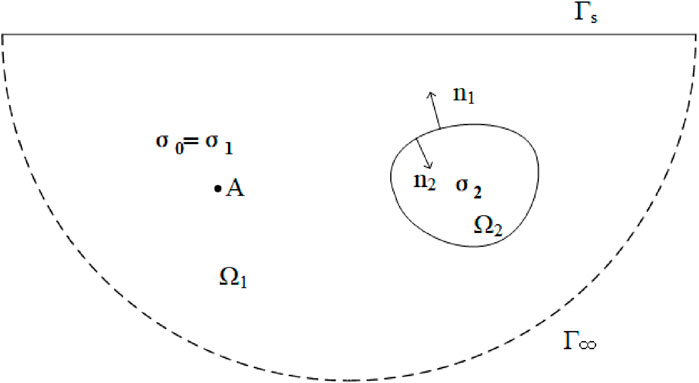
Figure 1. Geoelectric section of an inhomogeneous body (Xu, 1994). A is the point power supply,
The boundary value problem satisfied by the abnormal potential of the three-dimensional point source field is transformed into a variational problem (Equation 12):
2.4 Equivalent resistivity method
The forward calculation of the polarizability is found by the equivalent resistivity. When induced polarization effects are not considered, the value of the primary field potential
2.5 Three-dimensional forward theory of the cross-well induced polarization method based on the finite element method
As shown in Figure 2,
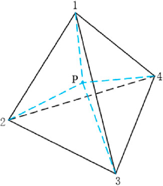
Figure 2. Tetrahedral element. P is the center of the tetrahedron, and 1, 2, 3, and 4 are vertex numbers respectively.
The shape function and its coefficients can be expressed as follows (Equations 20, 21):
When performing anisotropic forward, conductivity is the tensor form. Tetrahedral mesh to discrete equations. By integrating the four terms in the variational problem using the abnormal potential method in Equation 12, we can obtain the following equation (Equation 22).
If Equation 22 is changed to zero, we can obtain the following equation (Equation 23):
Likewise, polarizability anisotropy is based on the principle of the equivalent resistivity method. Its partial differential equation discretization is consistent with the resistivity method.
In this paper, an improved symmetric step-by-step over-relaxation preconditioned conjugate gradient iterative algorithm (SSOR-PCG) (Lin, 1998) is used. The matrix of coefficient A of the linear equations Ax=b is an n-order symmetric positive definite matrix, and the splitting matrix of the symmetric step-by-step over-relaxation iteration (SSOR method) is used as the pretreatment matrix M (Equation 24):
where D is the diagonal matrix of A, which is a strictly lower triangular matrix with L as A.
In Figure 1, when the point power is underground and the underground
R is the distance from the measuring point to the point current source A, and R’ is the distance from the measuring point to the imaginary point current source A’.
3 Algorithm validation
3.1 Three-dimensional complex isotropic cross-well sphere model
To verify the accuracy of the code written in this study, the cross-well sphere model in a homogeneous isotropic medium is used for verification (Xiong et al., 2016). The model shown in Figure 3 is established. The well spacing is 30 m, and the underground body is a low-resistivity sphere. Source point A supplies power at a depth of 20 m in well 1. There are 50 measuring points within every 1 m from 1 to 50 m in well 2. The resistivity of the sphere is 1 Ω·m, the radius of the sphere is 1 m, the burial depth of the center of the sphere is 20 m, the distance between the two wells is 15 m, and the resistivity of the surrounding rock is 100 Ω·m. The results calculated in this paper are compared with the analytical solutions calculated by Xiong et al. (2016).
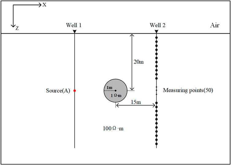
Figure 3. Schematic diagram of the three-dimensional complex isotropic cross-well sphere model. The emission source is located 20 m in Well 1. There are 50 measuring points in Well 2. The distance between the center of low-resistance sphere (1 Ω·m) and Well 2 is 15 m, and the surrounding rock resistivity is 100 Ω m.
As shown in Figure 4, the results calculated using the proposed algorithm are in good agreement with those calculated by Xiong et al. (2016), with a maximum relative error of 0.096% and an average relative error of 0.079%. The correctness and validity of the algorithm are verified, which also demonstrates the accuracy of the subsequent analysis of the results presented in this paper.
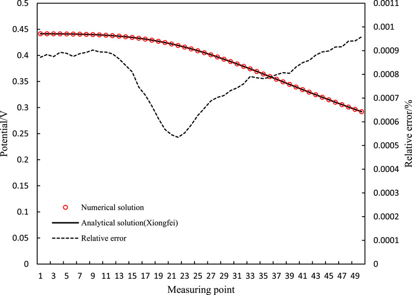
Figure 4. Comparison of the numerical solution and analytical solution. The red circle is the numerical solution curve, the black solid line is the analytical solution curve, and the black dotted line is the error curve.
3.2 Three-dimensional anisotropic model
To further validate the correctness of the proposed algorithm, a 3-D anisotropic model was created (Figure 5) (Xiong et al., 2023). In the model, the anomaly is a 100 m × 100 m × 100 m cube, the burial depth of the center of the anomaly is 55 m, and the size of the surrounding rock is 6,000 m × 6,000 m × 3,000 m. The conductivity of the surrounding rock is
As shown by the curve in Figure 6, this algorithm matches the results calculated by Xiong et al. (2023) well, with a maximum relative error of −1.1%. This verifies the correctness and validity of this algorithm and also indicates the accuracy of the subsequent analysis of the results presented in this paper.
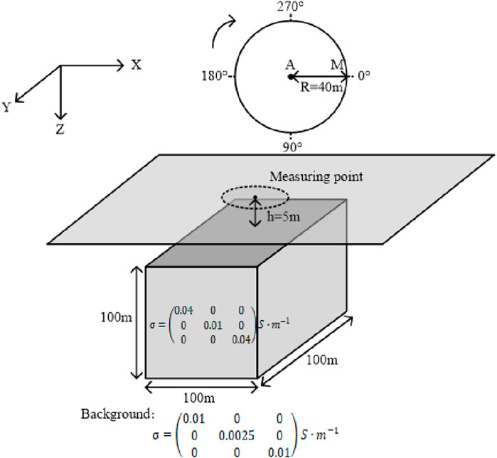
Figure 5. 3-D anisotropic model. The survey line is a circle with a radius of 40 m on the ground, and the abnormal body is a cube with a side length of 100 m and a depth of 5 m underground.
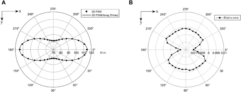
Figure 6. Curve plots of the apparent resistivity (A) and relative error (B) for the different algorithms of three-dimensional anisotropy. The point is the apparent resistivity of 3D FEM algorithm, and the line is the apparent resistivity curve of 3D FEM (Xiong Zhitao) algorithm.
4 Study of IP response between wells in electrically anisotropic media
To study the response of the induced polarization method for different cross-well geological models with conductivity and polarizability are anisotropic in different principal axis directions for abnormal bodies, a cross-well model (Figure 7) is designed. The abnormal bodies are divided into horizontal plate bodies and inclined plate bodies, and the inclined plate bodies are formed by rotating the horizontal plate bodies counterclockwise by 45°. The distance between the wells is 400 m, and three emitter sources A1, A2, and A3 are located at depths of 400, 600, and 800 m, respectively, in the wells. The center of the anomaly body is 600 m deep; the center is 200 m away from the measuring well, and the scale is 100 m × 100 m × 50 m (in the X, Y, and Z directions). The survey lines in well 2 are vertically arranged in a straight line. The first measurement point is located at the wellhead, and the last measurement point is located 1,200 m below the wellhead, with a total of 601 measurement points. The observed electrode system is a bipolar device.
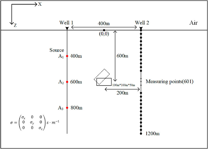
Figure 7. Schematic diagram of the cross-well induced polarization logging model. The emission sources are located at 400 m, 600 m, and 800 m in Well 1. There are 601 measuring points in Well 2, and the distance between adjacent measuring points is 2 m. The depth of 600 m between the two wells is a horizontal plate-like body (dotted line is inclined plate-like body) of 100 m * 100 m * 50 m.
Regarding the mesh dissection, to better fit the complex cross-well model, a free tetrahedral mesh is used. To improve the accuracy, the mesh size is reduced, and the numbers of the meshes at the emission source, survey line and abnormal body are increased. To achieve a better mesh dissection effect and to obtain more accurate calculation results, mesh processing is also carried out at the boundary. The results of different anomalies after the completion of mesh dissection are presented in Table 1. A diagram of the specific mesh generation is presented in Figure 8.

Table 1. Mesh generation results for the different abnormal bodies. The results are horizontal plate and inclined plate respectively.
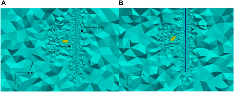
Figure 8. Diagram of the cross-well model mesh generation: (A) Horizontal plate-like body; and (B) inclined plate-like body. A1, A2, and A3 are excitation sources, yellow rectangular box is abnormal body, and blue line is borehole survey line.
4.1 The surrounding rock and the abnormal body are isotropic
To more effectively study and analyze the influence of the anisotropy, the response of the isotropy of the surrounding rock and anomalous body in different principal axis directions is analyzed in the research process, and the isotropic conductivity tensor of the surrounding rock and anomaly of the two cross-well geological models are set to be respectively:
Figures 9, 10 respectively show the anomaly curves of the isotropic apparent resistivity and apparent polarizability obtained from the forward calculation of the horizontal plates and inclined plates. Analyzing the cross-well IP response helps to understand the characteristics of the observed abnormal curves. The anomaly field caused by the horizontal plate-like body can be regarded as the combined effect of multiple electric dipole fields (Lv et al., 2012). The curves for the anomaly show the excitation characteristics of different depth emission sources in comparison to the anomaly and the excitation characteristics of the emitter sources for plate-like bodies with different inclinations. It can be seen that the curves of the apparent resistivity and apparent polarizability of the horizontal plate-like body are axisymmetric. In Figure 9, the emitter is close to the anomalous body at 600 m, the curve is most curved, and the values of the apparent resistivity and apparent polarizability reach the maximum at the center of the anomalous body. The maximum apparent resistivity and minimum apparent polarizability can be observed, and the curves exhibit a reverse stretching shape, which is caused by the emitter being close to the center of the anomalous body, the underground low resistivity body has obvious attraction to the current, and the current density is high; whereas the shallow and deep parts are far away from the emitter and anomalous body, and the current density is small. The extreme values of the apparent resistivity and apparent polarizability produced by the emitters at 400 and 800 m are near the bottom boundary and the top boundary, respectively, which are related to the position of the emitter. The emitter is located at the center of the anomalous body (at 600 m), so the extreme values are located at the center of the anomalous body. Similarly, because the abnormal body is rotated by 45°, the abnormal curves of the inclined plate-like body is roughly the same as that of the horizontal plate-like body, and the reason for this is the same as in the case of the horizontal plate-like body. Different from the horizontal plate-like body, the inclined plate-like body causes the absolute values of the apparent resistivity and apparent polarizability of the emitters at different positions to decrease to a certain extent and has the greatest influence on the emitters at a shallow depth of 400 m. Because of the inclination of the plate-like body, the positions of all of the extreme values of the response curves are shifted upward and the variations in the amplitude of the curves become wider to a certain extent.
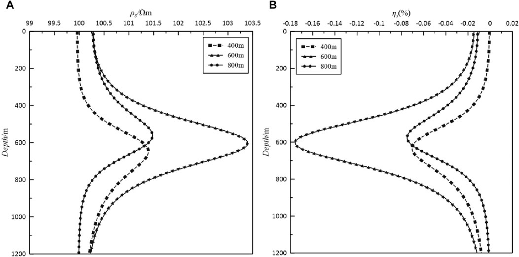
Figure 9. Graphs of the (A) apparent resistivity and (B) apparent polarizability of the isotropic horizontal plate-like body. The response curves with squares are the results for 400 m excitation sources, the response curves with triangles are the results for 600 m excitation sources, and the response curves with dots are the results for 800 m excitation sources.
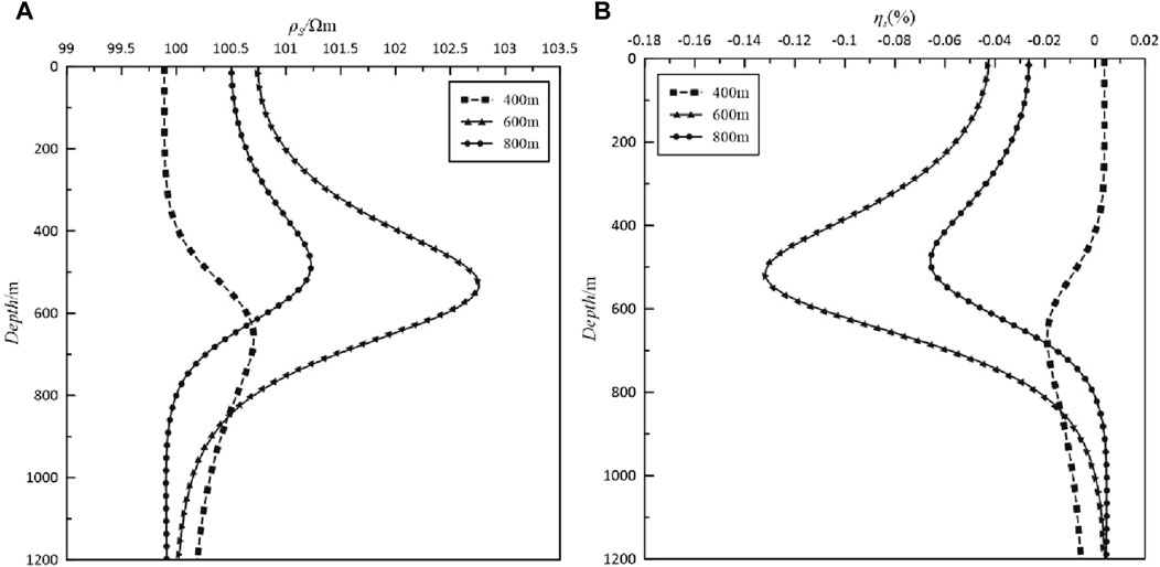
Figure 10. Graphs of the (A) apparent resistivity and (B) apparent polarizability of the isotropic inclined plate-like body. The response curves with squares are the results for 400 m excitation sources, the response curves with triangles are the results for 600 m excitation sources, and the response curves with dots are the results for 800 m excitation sources.
Therefore, the response of the isotropic surrounding rock and abnormal body has been analyzed. A good foundation for analyzing the anisotropy of the conductivity and polarizability of the abnormal body.
4.2 Polarizability is isotropic and conductivity is anisotropic of abnormal body
To better analyze the influence of the anisotropy of the anomalous bodies conductivity on the apparent resistivity and apparent polarizability, it is assumed that the anomalous bodies polarizability is isotropic and the anomalous bodies conductivity is anisotropic in different principal axis directions. In addition, the anisotropic conductivity tensors of the two modeled anomalous bodies are set as
Figure 11 shows the response curves of the apparent resistivity and apparent polarizability produced by the emission sources at different positions under the condition of anisotropic conductivity for the horizontal plate-like body. As can be seen from Figure 11, the effect of x-direction anisotropic conductivity is maximized regardless of the location of the emission source for the apparent resistivity response curves, and the conductivity of the x-direction anisotropy greatly reduces the apparent resistivity compared to the isotropic condition. The extreme positions of the apparent resistivity curves for the emission sources at 400 and 800 m shift downward and upward, respectively, compared with that for the emission source at 600 m. Compared to the apparent resistivity curve, the apparent polarizability curve has more obvious changes. The x-direction anisotropic conductivity causes the extreme absolute value of the apparent polarizability to greatly increase compared with the isotropy. It should be noted that the extreme position of the apparent polarizability is near 600 m regardless of the position of the emitter. The apparent polarizability curve of the y-direction anisotropic conductivity is basically consistent with the response curve for the isotropic condition and is independent of the position of the emission source. The apparent polarizability curve of the z-direction anisotropic conductivity exhibits obvious characteristics and is related to the position of the emitter. When the emitter and plate are located at the same depth, the absolute value of the apparent polarizability only slightly increases. When the emitter is located at 400 and 800 m, the absolute value of the extreme value of the apparent polarizability increases, and the position shifts downward for the emitter located at 400 m and upward for the emitter located at 800 m.
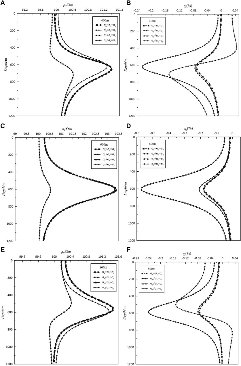
Figure 11. Curves of the anisotropy of the conductivity of the horizontal plate-like body (left (A,C,E): apparent resistivity, and right (B,D,F): apparent polarizability). The response curves with squares are the results of isotropic anomalies, the response curves with dots are the results of anisotropic anomalies of conductivity in the x-direction, the response curves with triangles are the results of anisotropic anomalies of conductivity in the y-direction, and the response curves with rhombuses are the ones of anisotropic anomalies of conductivity in the z-direction.
Figure 12 presents the response curves of the apparent resistivity and apparent polarizability produced by the emission sources at different locations under the anisotropic conductivity condition for the inclined plate-like body. The curves of the apparent resistivity and apparent polarizability at y-direction anisotropy are consistent with the isotropic characteristics, but the extreme value decreases and the position shifts upward compared with the horizontal plate-like body. The anisotropic response characteristic in the z-direction is more distinct. The inclination of the plate-like body causes the extreme value of the z-direction anisotropic apparent resistivity to be less than the isotropy at the 600 and 800 m emitters, and the extreme value shifts downward. However, the extreme value of the apparent resistivity at the location of the 400 m emitter is greater than the isotropy, and its position shifts upward. The apparent polarizability also changes obviously at the locations of the 600 and 800 m emitters. Compared to the horizontal plate-like body, the absolute value of the extreme value of the apparent polarizability increases and its position shifts upward.
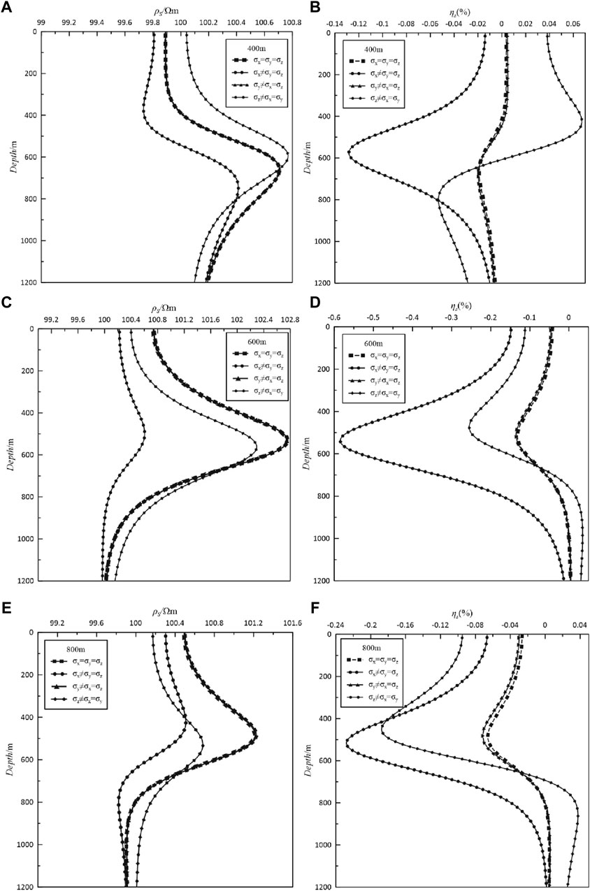
Figure 12. Curves of the anisotropy of the conductivity of the inclined plate-like body (left: (A,C,E) apparent resistivity, and right: (B,D,F) apparent polarizability). The response curves with squares are the results of isotropic anomalies, the response curves with dots are the results of anisotropic anomalies of conductivity in the x-direction, the response curves with triangles are the results of anisotropic anomalies of conductivity in the y-direction, and the response curves with rhombuses are the results of anisotropic anomalies of conductivity in the z-direction.
4.3 Polarizability is anisotropic and conductivity is isotropic of abnormal body
To better analyze the effects of the anisotropy of the anomaly’s polarizability on the apparent resistivity and apparent polarizability, it is assumed that the conductivity of the anomalous body is isotropic and the polarizability of the anomalous body is anisotropic in different principal axis directions. The anisotropy polarizability tensors of the two models are
Figure 13 presents the apparent polarizability response curves for the horizontal plate-like body when the polarizability is anisotropic in different principal axis directions. It can be seen from the diagrams for the three different emission source models that the x-direction anisotropic polarizability has the greatest influence on the apparent polarizability, which leads to a significant decrease in the extreme absolute value of the apparent polarizability at the center of the abnormal body, and the absolute values of the apparent polarizability in the upper and lower parts of the abnormal body are reduced to a certain extent. The responses of the apparent polarizability for anisotropy and isotropy of polarizability in the y-direction are almost the same, and it only increases slightly at the minimum position. When the polarizability is anisotropic in the z-direction, the apparent polarizability of the emitter model at 600 m is similar to that in the isotropic case, and it increases slightly at the minimum position. The apparent polarizability only changes at 400 and 800 m. When the emitter is located at 400 m, the minimum value of the apparent polarizability at the center of the anomalous body increases slightly and the extreme center shifts upward. The apparent polarizability above the anomaly body is larger than that for the isotropic case, while the apparent polarizability below the anomaly body is smaller than that for the isotropic case. When the source is located at 800 m, the change in the apparent polarizability is the opposite to that when the source is located at 400 m.
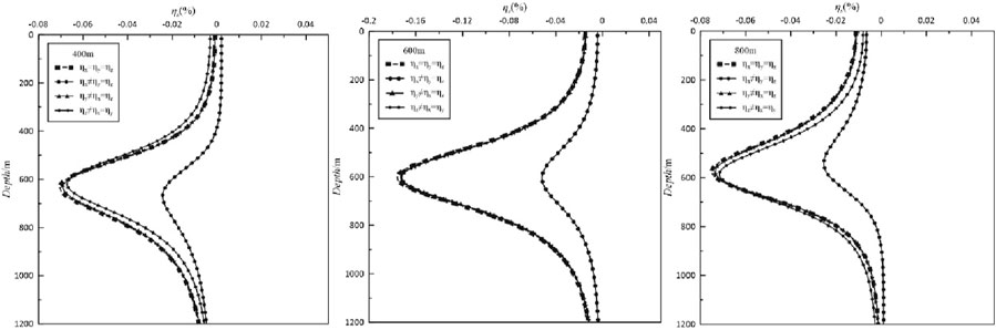
Figure 13. Curves of the anisotropic apparent polarizability for the horizontal plate-like body. The response curves with squares are the results of isotropic anomalies, the response curves with dots are the results of anisotropic anomalies of polarizability in the x-direction, the response curves with triangles are the results of anisotropic anomalies of polarizability in the y-direction, and the response curves with rhombuses are the results of anisotropic anomalies of polarizability in the z-direction.
Figure 14 presents the apparent polarizability response curves when the polarizability is anisotropic in different principal axis directions for the inclined plate. Compared with that for the horizontal plate, the apparent polarizability curves change greatly when the abnormal body is tilted. In particular, the anisotropy characteristics of the abnormal body are most obvious when excited at the upper and lower positions of the abnormal body is located at 400 and 800 m, respectively, and the response curves fluctuate strongly. Compared to the horizontal plate, the extreme position of the apparent polarizability curves of the x-direction anisotropic polarizability shifts downward and upward. The apparent polarizability curves of the y-axis anisotropic polarizability are basically the same as for the case in which the polarizability is isotropic, but the position of the extreme value is different from that for the horizontal plate-like body. When the polarizability is anisotropic in the z-direction, the extreme apparent polarizability of the emitter at 400 m is almost the same as that for the isotropic case, and the absolute values of the extreme apparent polarizability for the other two emitters decrease. Consistent with the anisotropic conductivity of the anomalous body, the inclination of the plate-like body causes the absolute value of the extreme apparent polarizability of the emitter to decrease greatly when the emitter is located at 400 m. For both the horizontal and inclined plate-like bodies, it was found that the absolute value of the apparent polarizability is the largest when the emitter is located at 600 m, that is, the response characteristics of the emitter located closest to the anomalous body are the most obvious when the emitter is located at 600 m.
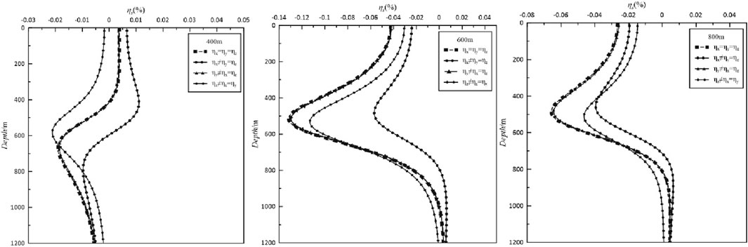
Figure 14. Curves of the anisotropic apparent polarizability anomaly for the inclined plate-like body. The response curves with squares are the results of isotropic anomalies, the response curves with dots are the results of anisotropic anomalies of polarizability in the x-direction, the response curves with triangles are the results of anisotropic anomalies of polarizability in the y-direction, and the response curves with rhombuses are the results of anisotropic anomalies of polarizability in the z-direction.
4.4 Conductivity and polarizability of abnormal body are anisotropic
To analyze the influences of the anisotropy of the conductivity and polarizability of the anomalous bodies on the apparent resistivity and apparent polarizability in the cross-well induced polarization method, the anisotropy tensors of the conductivity of the anomalous bodies in the two models are set as
Figure 15 presents the apparent polarizability response curves produced by the emitters located at different depths when the conductivity and polarizability of the horizontal plate-like body are anisotropic. Compared with the isotropic case, the responses of the apparent polarizability produced by the three different emitters for the x-direction and y-direction anisotropy exhibit similar change characteristics, and the absolute value of the apparent polarizability extremum increases, but the extreme value changes more when the x-direction anisotropy is greater than the y-direction anisotropy. When z-direction anisotropy is maintained at 600 m emission, the apparent polarizability extreme position is maintained near 600 m. Compared to the isotropic case, only the absolute value of the extreme value increases, and the variation characteristics are different at 400 and 800 m. Although both positions lead to an increase in the absolute value of the extreme value, the position of the extreme value shifts in the opposite directions. It shifts downward for the 400 m case and upward for the 800 m case. Figure 16 shows the curves of the response of the apparent polarizability produced by emitters located at different depths when the conductivity and polarizability of the inclined plate-like body are anisotropic. Compared to the horizontal plate-like body, the absolute value of the extreme value of apparent polarizability for the x-direction anisotropy increases more than that for the isotropic case, and the position of the extreme value shifts upward. For the y-axis and z-axis anisotropy, on the response curves of the emitter located at 800 m, the position of the extreme value shifts upward. When the emitter is located at 600 m, the position of the extreme value shifts upward and the absolute value of the extreme value decreases. When the emitter is located at 400 m, the change is greater. The inclination of the plate-like body controls the overall trend of change of the apparent polarizability curves. It should be noted that the electrical response curves for the y-axis anisotropy are basically consistent with the typical response curves for the isotropic case when the of the conductivity and polarizability is anisotropic in different principal axis directions or when the anomalous body is inclined.
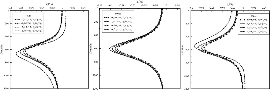
Figure 15. Curves of the anisotropic apparent conductivity and polarizability for the horizontal plate-like body. The response curves with squares are the results of isotropic anomalies, the response curves with dots are the results of anisotropic anomalies of conductivity and polarizability in the x-direction, the response curves with triangles are the results of anisotropic anomalies of conductivity and polarizability in the y-direction, the response curves with rhombuses are the results of anisotropic anomalies of conductivity and polarizability in the z-direction.
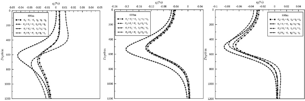
Figure 16. Curves of the anisotropic apparent conductivity and polarizability for the inclined plate-like body. The response curves with squares are the results of isotropic anomalies, the response curves with dots are the results of anisotropic anomalies of conductivity and polarizability in the x-direction, the response curves with triangles are the results of anisotropic anomalies of conductivity and polarizability in the y-direction, the response curves with rhombuses are the results of anisotropic anomalies of conductivity and polarizability in the z-direction.
5 Conclusion
(1) Through forward response calculations and analysis of the electrical anisotropic models of horizontal and inclined plate-like bodies, it was found that for the cross-well induced polarization method, when the electrical properties of plate-like bodies are isotropic in different principal axis directions, the extreme values of absolute values of the apparent resistivity and apparent polarizability of the emission source at 600 m are the maximum due to the attraction of the underground low resistivity to the current. There are many differences in the positions where the extreme values of the electrical curves appear due to the different positions of the emitters. When the plate-like body is inclined, the amplitudes of all of the curves decrease and shift upward.
(2) When the conductivity is anisotropic in different principal axis directions, for the horizontal plate-like body, the x-direction anisotropic conductivity has the greatest influence on the electrical characteristics and the apparent polarizability is more obvious than the apparent resistivity. In addition, the position of the emitter has an obvious influence on the apparent polarizability when the conductivity is anisotropic in z-direction. The inclination of the plate-like body causes the apparent resistivity and apparent polarizability curves to have different effects, but the extreme values of the absolute values of the apparent resistivity and apparent polarizability will decrease.
(3) When the polarizability is anisotropic in different principal axis directions, for the horizontal plate-like body, only the x-direction anisotropy has an obvious effect on the apparent polarizability curve. The y-direction and z-direction anisotropy has the same apparent polarizability curve as that for the isotropic case. The inclination of the plate-like body causes the apparent polarizability curve to change greatly. In particular, when excited at 400 m and 800 m, the anisotropy characteristics of the anomalous body are most obvious, and the response curves fluctuate strongly.
(4) When the conductivity and polarizability of the plate-like body are anisotropic, the responses of the apparent polarizability of the horizontal plate-like body when the x-direction and y-direction anisotropy are similar to those for the isotropic case, while z-direction anisotropy has a more complex influence. The inclination of the plate-like body causes the extreme position of the x-direction anisotropic apparent polarizability to shift upward. For y-direction and z-direction anisotropy, when the emitter is located above the inclined plate-like body, the overall change trend of the apparent polarizability curves decreases. It was found that for the induced polarization method, the response in a borehole is complex and changeable, and the inclination of the abnormal body also affects the response. The results of this study provide theoretical support for the study of the anisotropy of induced polarization in boreholes. In this paper, inversion is conducted to further verify and expand the forward work, so subsequent inversion work was very necessary for this study.
Data availability statement
The original contributions presented in the study are included in the article/supplementary material, further inquiries can be directed to the corresponding author.
Author contributions
ZJ: Writing–original draft. ZL: Writing–review and editing. WX: Writing–review and editing. XX: Writing–review and editing. MY: Writing–review and editing. YL: Writing–review and editing.
Funding
The author(s) declare that financial support was received for the research, authorship, and/or publication of this article. This study was funded by the National Natural Science Foundation of China (42030805 and 42274103).
Conflict of interest
The authors declare that the research was conducted in the absence of any commercial or financial relationships that could be construed as a potential conflict of interest.
Publisher’s note
All claims expressed in this article are solely those of the authors and do not necessarily represent those of their affiliated organizations, or those of the publisher, the editors and the reviewers. Any product that may be evaluated in this article, or claim that may be made by its manufacturer, is not guaranteed or endorsed by the publisher.
References
Arato, A., and Godio, A. (2014). Staggered grid inversion of cross hole 2-D resistivity tomography. J. Appl. Geophys. 107, 60–70. doi:10.1016/j.jappgeo.2014.05.004
Deng, B., and Li, J. Z. (2014). Application effect of borehole geophysical prospecting method in metal ore exploration. Sichuan J. Geol. 34 (02), 276–280.
Di, Q. Y., and Wang, M. Y. (1997). Preliminary study on current line tracing potential resistivity tomography. Adv. Geophys. (04), 27–35.
Dong, Q. H., and Zhu, J. S. (1999). Cross-well resistivity tomography and its application. Comput. Phys. (05), 474–480. doi:10.19596/j.cnki.1001-246x.1999.05.004
Feng, J., Liu, T. Y., Yang, Y. S., and Gao, W. L. (2010). Combined inversion technology of 3D borehole geomagnetic survey and its application. J. Adv. Geophys. 25 (05), 1685–1691.
Harold, O. S. (1959). Mathematical formulation and type curves for induced polarization. Geophysics 24 (3), 547–565. doi:10.1190/1.1438625
Hou, J., Mallan, R. K., and Torres-Verdi, N. (2006). Finite-difference simulation of borehole EM measurements in 3D anisotropic media using coupled scalar-vector potentials. Geophysics 71 (5), G225–G233. doi:10.1190/1.2245467
Hu, D., Yang, X., Yue, M., Li, Y., and Wu, X. (2021). Prediction model for advanced detection of water-rich faults using 3D anisotropic resistivity modeling and Monte Carlo methods. IEEE Access 9, 18251–18261. doi:10.1109/access.2021.3053861
Hu, D. M., Tezkan, B., Niu, H., Yue, M., Yang, X., and Wu, X. (2023). 3D time-domain induced polarization modelling considering anisotropy and topography. J. Appl. Geophys. 208, 104871. doi:10.1016/j.jappgeo.2022.104871
Kenkel, J., Hördt, A., and Kemna, A. (2012). 2D modelling of induced polarization data with anisotropic complex conductivities. Near Surf. Geophys. 10 (6), 533–544. doi:10.3997/1873-0604.2012050
Lin, S. Z. (1998). Solving finite element equations by preconditioned conjugate gradient method and programming. J. Hohai Univ. (03), 114–117.
Linde, N., and Pedersen, L. B. (2004). Evidence of electrical anisotropy in limestone formations using the RMT technique. Geophysics 69 (4), 909–916. doi:10.1190/1.1778234
Liu, G. Q., Tao, G., Ke, S. Z., Yang, H. Z., and Jiang, J. Y. (2001). A perturbation method for resistivity tomography of Frechet derivative. Seismol. Geol. (02), 314–320.
Liu, Y. Z., Yin, C. C., Cai, J., et al. (2018). Present situation and prospect of anisotropy research in electromagnetic exploration. J. Geophys. 61 (08), 3468–3487.
Lv, Y. Z., Ruan, B. Y., and Huang, J. G. (2003). The 3-D immediate Cross hole tomography with direct current. Geophys. Geochem. Comput. Tech. (01), 60–64.
Lv, Y. Z., Ruan, B. Y., and Peng, S. P. (2012). Study on anomaly characteristics of ground-well azimuth IP observation. Adv. Geophys. 27 (01), 201–216. doi:10.6038/j.Issn.1004-2903.2011.06.023
Mcmonnies, B. (2007). “Ground geophysics and borehole logging-A decade of implements,” in Exploration in the New Millennium: Proceedings of the Fifth Decennial International Conference on Mineral Exploration, pp. 39–49.
Mi, H. Z. (2019). Research status and development of underground geophysical exploration technology for metal deposits. Mineral. Explor. 10 (03), 601–605.
Pek, J., and Santos, A. M. (2006). Magnetotelluric inversion for anisotropic conductivities in layered media. Phys. Earth and Planet. Interiors 158 (2-4), 139–158. doi:10.1016/j.pepi.2006.03.023
Schmutz, M., Albouy, Y., Guérin, R., Maquaire, O., Vassal, J., Schott, J. J., et al. (2000). Joint electrical and time domain electromagnetism (TDEM) data inversion applied to the Super Sauze earthflow (France). Surv. Geophys. 21, 371–390. doi:10.1023/a:1006741024983
Shima, H. (1987). Resistivity tomography: an approach to 2-Dreistivity inverse problems. Ann.internat.mtg.soc.expl.geophys.expanded Abstr. (1), 59–61. doi:10.1190/1.1892038
Stolz, E. M. (2000). Electromagnetic methods applied to exploration for deep nickel sulphides in the Leinster area, Western Australia. Explor. Geophys. 31 (2), 222–228. doi:10.1071/eg00222
Wang, Q. Y., and Hu, Y. P. (2004). Thoughts on the shortage of metal resources and prospecting for concealed deposits. J. Geol. Explor. 2004 (06), 75–79.
Wang, T. (2002). The electromagnetic smoke ring in a transversely isotropic medium. Geophysics 67, 1779–1789. doi:10.1190/1.1527078
Wang, Z. (2015). Forward and inversion of IP in borehole and its application. Wuhan, China: China University of Geosciences.
Xiong, F., Lv, Y. Z., and Li, Y. (2016). Study on 2.5-dimensional approximate imaging of well-well resistivity. Geophys. Geochem. Calc. Technol. 38 (03), 308–313.
Xiong, P. (2004). Progress and prospect of geophysical prospecting technology in China. Pet. Geophys. Explor. (03), 354–358.
Xiong, Z. T., Tang, X. G., and Li, D. D. (2023). Arbitrarily anisotropic forward modeling of the 3D borehole-to-surface resistivity method based on unstructured grid finite element. Chin. J. Geophys. 66 (05), 2201–2218. doi:10.6038/cjg2022Q0830
Yan, Y. J., Zhou, L., Xie, X. B., and Wang, Z. G. (2014). Transient electromagnetic response of reservoir electrical anisotropy model. J. Eng. Geophys. 11 (03), 346–350. doi:10.3969/j.issn.1672-7940.2014.03.013
Yin, C. C. (2010). Geoelectrical inversion for a one-dimensional anisotropic model and inherent non-uniqueness. Geophys. J. Int. 140 (1), 11–23. doi:10.1046/j.1365-246x.2000.00974.x2000.00974.X
Yu, A. J., Huang, H., Xu, D. L., Fan, Z. J., and Chen, X. Q. (2006). Application of comprehensive electrical method in searching for concealed deposits in Haxi gold mining area, Xinjiang. Geol. Explor. (06), 57–61.
Yuan, G. Q., Xiong, S. Q., Meng, Q. M., et al. (2011). Research on geophysical exploration technology and application. J. Geol. 85 (11), 1744–1805.
Zhdanov, M. S., and Yoshioka, K. (2003). Cross-well electromagnetic imaging in three dimensions. Explor. Geophys. 34 (2), 34–40. doi:10.1071/eg03034
Zhou, P., Chen, S. L., and Zhu, L. L. (2009). Review of several underground geophysical prospecting methods for metal deposits. Geol. Bull. 28 (Z1), 224–231.
Keywords: cross-well induced polarization method, anisotropy, finite element method, conductivity and polarizability, three-dimensional forward
Citation: Junke Z, Lei Z, Xinyu W, Xingbing X, Yurong M and Liangjun Y (2024) Study of response characteristics of cross-well induced polarization method in anisotropic media. Front. Earth Sci. 12:1443764. doi: 10.3389/feart.2024.1443764
Received: 04 June 2024; Accepted: 08 August 2024;
Published: 21 August 2024.
Edited by:
Bo Yang, Zhejiang University, ChinaCopyright © 2024 Junke, Lei, Xinyu, Xingbing, Yurong and Liangjun. This is an open-access article distributed under the terms of the Creative Commons Attribution License (CC BY). The use, distribution or reproduction in other forums is permitted, provided the original author(s) and the copyright owner(s) are credited and that the original publication in this journal is cited, in accordance with accepted academic practice. No use, distribution or reproduction is permitted which does not comply with these terms.
*Correspondence: Zhou Lei, NTAxMTYxQHlhbmd0emV1LmVkdS5jbg==