 Xiao Liu
 Shijie Gao
- 1School of Hydraulic and Electric-power, Heilongjiang University, Harbin, China
- 2Institute of Geophysics, China Earthquake Administration, Beijing, China
Considering the significant impact of anisotropy on forward and inversion results, this paper presents a research study on tensor controlled-source audio magnetotellurics (CSAMT) forward modeling in axis anisotropic media. In this study, the tensor resistivity of axis anisotropic medium is introduced according to the control equation of electric field with sources. The total electric field is decomposed into primary and secondary fields, with the primary field obtained using Key’s algorithm and the secondary field calculated using the finite difference method. This approach enables three-dimensional (3D) modeling of tensor CSAMT in axis anisotropic media. The correctness of the algorithm is verified by comparing it with the results obtained using a two-dimensional (2D) finite element algorithm. Several sets of axis anisotropic 3D models are designed, and the response characteristics of anisotropic target bodies to plane waves and non-plane waves are summarized. The findings indicate that the Cagniard resistivity and tipper are sensitive to changes in the X and Y directions of the anomaly, but not sensitive to changes in resistivity in the Z direction. Additionally, in the near region, non-plane wave CSAMT signals may cause distortion in the Cagniard resistivity. The results highlight that tensor CSAMT has the capability to detect changes in resistivity in two-axis directions (X and Y), providing greater exploration advantages compared to scalar CSAMT. This study provides a foundation for the forward modeling and inversion of tensor CSAMT in arbitrary anisotropic media.
1 Introduction
Controlled-source audio magnetotellurics has the advantages of high work efficiency and high signal-to-noise ratio. CSAMT has been widely used in fields such as geological exploration, oil, natural gas, geothermal, metal mineral exploration, and hydrological and environmental engineering fields (Xue et al., 2015; Guo et al., 2019; Xu et al., 2020; Di et al., 2020).
Scalar CSAMT can be divided into equatorial and axial devices. Both use a field source to excite and collect two components (
Among the factors that directly affect the results of forward modeling and inversion, anisotropy has a significant impact. Considering that anisotropy is very common in areas with well-developed stratigraphic layers, it is necessary to develop electromagnetic data processing and inversion methods in anisotropic media to improve the accuracy of inversion and the level of geological interpretation (Liu et al., 2018). The use of electrical anisotropy information can deepen our understanding of the structure of the Earth’s lithosphere, the laws of material transport in deep Earth, and the dynamic processes in deep Earth (Kirkby et al., 2015).
Yin et al. (2014) performed a 3D forward modeling study of marine controlled-source electromagnetic method using a staggered finite difference technique to analyze the influence of seabed conductivity anisotropy on shallow sea data. Cai et al. (2015) used the scalar finite element method to obtain the response of CSAMT with anisotropic conductivity. Li et al. (2017) and He et al. (2019) applied the vector finite element method to achieve anisotropic forward modeling of CSAMT. These studies showed the significant impact of axis anisotropic tensor conductivity on the response results of CSAMT, especially the amplitude and distribution characteristics of apparent resistivity (Qiu et al., 2018).
There have been relatively few studies on tensor CSAMT forward modeling and inversion on axis anisotropic media (Wang K. P. et al., 2018; Liu and Zheng, 2024). No research results on tensor CSAMT forward modeling and inversion of arbitrary anisotropy have been published. Wang and Tan et al. (2017) and Wang et al. (2017) demonstrated through finite difference forward modeling that tensor CSAMT can identify at least two horizontal resistivities through multi-component observations, and provides some help for the preliminary qualitative interpretation of tensor CSAMT. Their research focused on how to achieve axis anisotropic inversion.
Based on the study of isotropic media, this study applies the finite difference method (Xie et al., 2016) to tensor CSAMT research on axis anisotropy, analyzes the influence of axis anisotropy on the forward modeling results of tensor CSAMT, and summarizes the response characteristics of anisotropic target bodies with plane waves and non-plane waves. The study provide a foundation for the forward modeling and inversion of tensor CSAMT in arbitrary anisotropic media.
2 Forword modeling method
2.1 Finite difference method for calculating electromagnetic fields
For isotropic media, ignoring displacement current, under the excitation condition of an electrical source, the electric field
where
The total field
In axis anisotropic media, the tensor conductivity is
Substitute Equation 3 into Equation 2 and organize it to obtain the following equation for the three components of the electric field:
The calculation method for the electric field
where
Set the secondary field values at the top boundary, four side boundaries, and underground bottom boundary of the study area to zero as the boundary condition. The quasi minimum residual (QMR) method is used to solve Equation 7, and divergence correction is introduced during the iteration process (Siripunvaraporna et al., 2002; Liu and Sun, 2024), to obtain the three component values of the electric field in the entire space. Interpolation method is used to calculate the electromagnetic field components values of measurement points on the surface.
2.2 Calculating tensor impedance and tipper
Tensor CSAMT is excited by two field sources with different polarization directions. This study uses a “+” shaped orthogonal field source to excite in two directions, that is, the forward calculation for each frequency requires solving Equation 7 twice. Collect five electromagnetic field components in the receiving area, denoted as
The expressions for the main diagonal impedance components and tipper are as follows:
The corresponding Cagniard resistivity equation is:
where
2.3 Algorithm validation
The algorithm is written in Fortran language. To verify the correctness of the algorithm, we designed a 2D model and compared it with the finite element method results of Key (2016). The background resistivity is 100
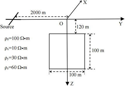
Figure 1. Sketch of 2D model.
The comparison of impedance results between the two methods is shown in Figure 2. The real and imaginary parts of
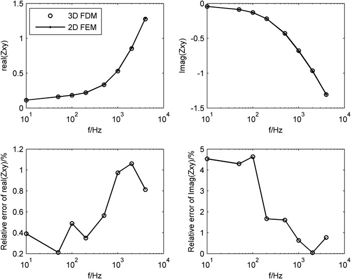
Figure 2. Comparison of the results of 3D FDM and 2D FEM results.
3 Forward modeling case
3.1 Response characteristics of low-resistance model
The 3D low-resistance prism model is shown in Figure 3, with a background resistivity of 100
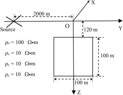
Figure 3. Sketch of the 3D model.
The centers of two intersecting ground wire sources are located at −2,000 m on the Y-axis, with a length of 100 m and angle of 45° and 135° with the Y-axis, respectively. The transmission frequency is 500 Hz. The finite difference mesh is 33 × 42 × 41 (including 12 air layers).
The forward results of the low-resistance model are shown in Figure 4. It is evident that the Cagniard resistivity
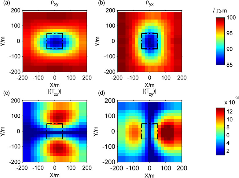
Figure 4. Response of the 3D model. (A)
3.2 Influence of anisotropy on response characteristics
The study by Wang et al. (2017) demonstrated that when the resistivity of the axis anisotropic model in the X direction is the same as that of the isotropic model, the apparent resistivity of the XY-mode is almost the same. When the resistivity of the axis anisotropic model in the Y direction is the same as that of the isotropic model, the apparent resistivity of the YX-mode in both models are almost the same. To illustrate the impact of changes in the axis anisotropy of low-resistance bodies on the forward response, we established three sets of axis anisotropy resistivity models (Table 1) to simulate the resistivity changes of anomalous bodies in the X, Y, and Z directions.
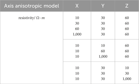
Table 1. The axis anisotropic model.
The size of the low-resistance model and the parameters of the source are the same as the example in section 3.1.
The transmission frequency of the source is 500 Hz. At this time, the CSAMT signal is approximately a plane wave. We first fix the resistivity of the low-resistance body in the Y and Z directions to 30 and 60
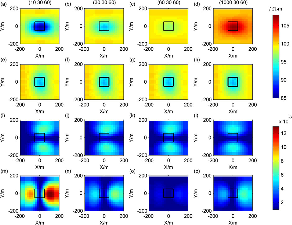
Figure 5. Contour maps of response of different resistivity in the X direction: (A–D)
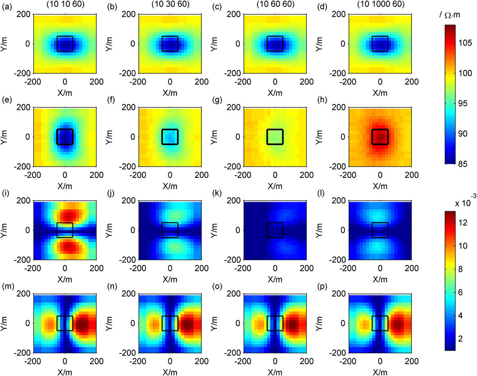
Figure 6. Contour maps of response of different resistivity in the Y direction: (A–D)
Figure 7. Contour maps of response of different resistivity in the Z direction: (A–D)
The Cagniard resistivity
Similarly,
In CSAMT, in the XY-mode, the polarization direction of the electric field is mainly in the X direction, making it sensitive to the electrical resistivity of the low-resistance body in the X direction. In the YX-mode, the polarization direction of the electric field is primarily in the Y direction, making it sensitive to the resistivity of low-resistance bodies in the Y direction.
3.3 Impact of model size on response characteristics
To illustrate the impact of changes in model size on forward response, we set up three sets of axis anisotropic resistivity models (Table 2), to represent the length, width, and height changes of anomalous bodies in the X, Y, and Z directions, respectively. The resistivity in the X, Y, and Z directions are 10, 30, and 60
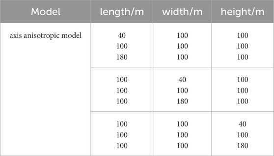
Table 2. Axis anisotropic low-resistance model.
We first fix the width and height of the low-resistance body to 100 m, with the length in the X direction of 40, 100, and 180 m, respectively, the forward results are shown in Figure 8. Next, we fix the length and height of the low-resistance body to 100 m, with the width in the Y direction of 40, 100, and 180 m, respectively, the forward results are shown in Figure 9. Finally, we fix the length and width of the low-resistance body to 100 m, with the height in the Z direction of 40, 100, and 180 m, respectively, the forward results are shown in Figure 10.
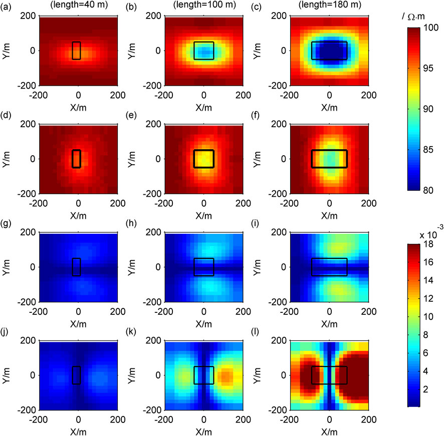
Figure 8. Contour maps of response when the length of model changes: (A–C)
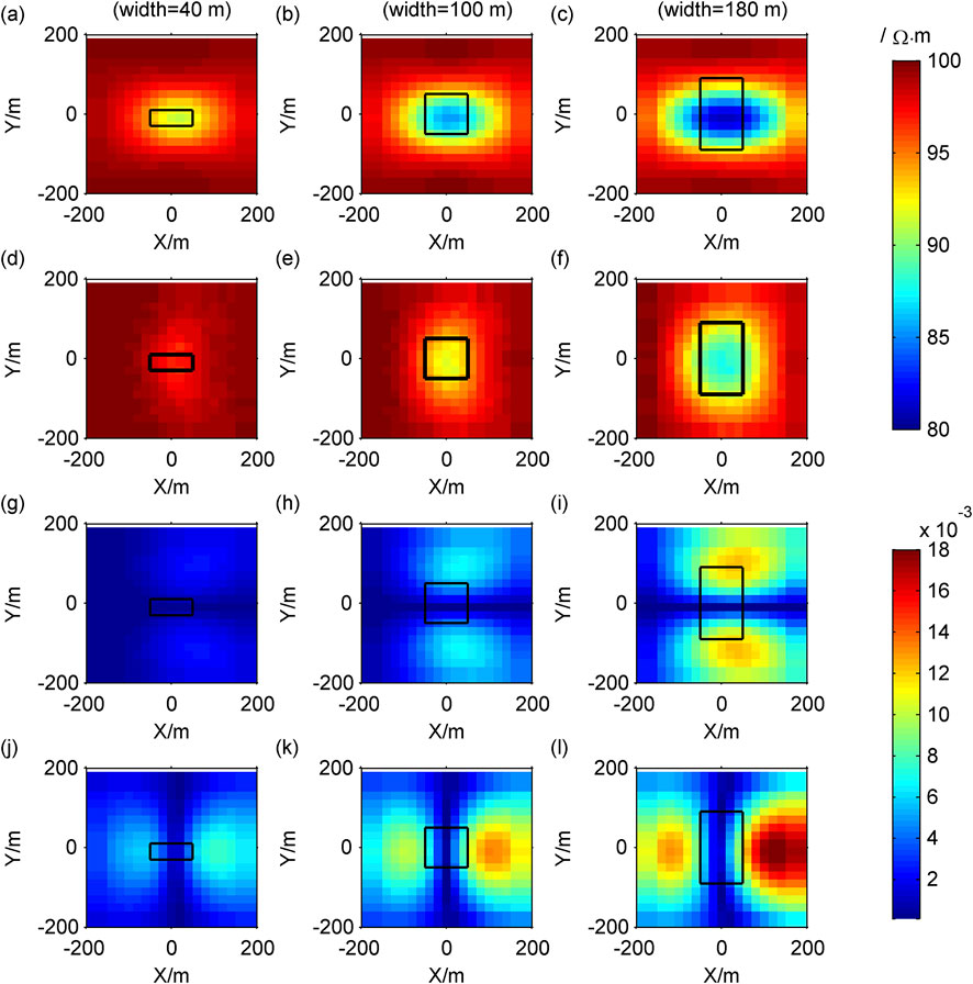
Figure 9. Contour maps of response when the width of the model changes: (A–C)
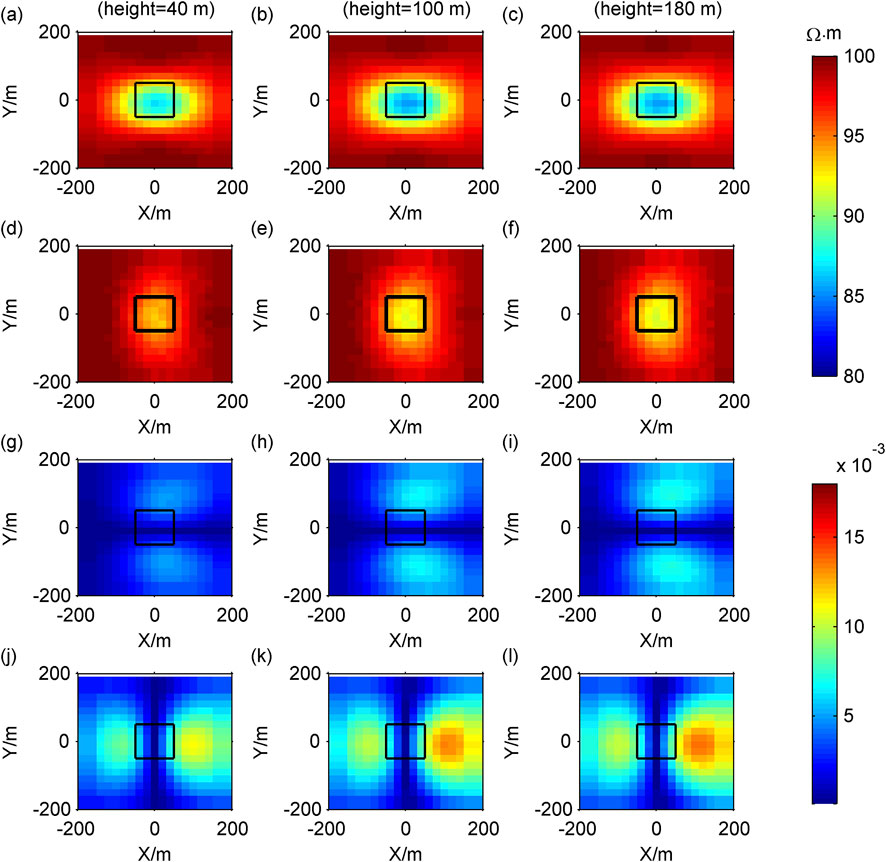
Figure 10. Contour maps of response when the width of the model changes: (A–C)
As the length, width and height of the anomalous body increase, both the modulus of Cagniard resistivity anomaly and the modulus of tipper increase, leading to an expansion of the anomalous area (Figures 8–10).
The boundary of the
3.4 Response of axis anisotropic complex prism model
Here, a prism model is established with a top burial depth of 120 m. The plan of the model is shown in Figure 11, and the resistivity in the X, Y, and Z directions is 10, 1,000, and 100
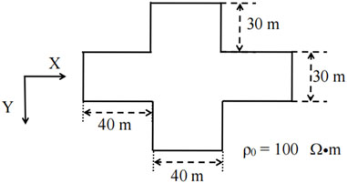
Figure 11. Sketch of 3D axis anisotropic prism model.
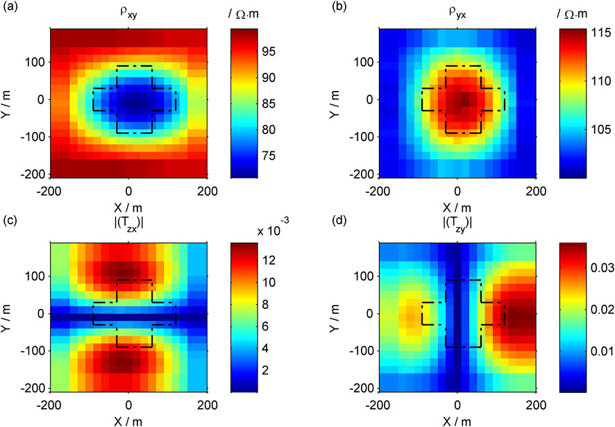
Figure 12. Response of the 3D anisotropic prism model. (A)
The low-value anomaly area in the contour map of
3.5 Response in non-plane wave areas
For case 3.2, when the transmission frequency of the source is 10 Hz, the receiving region belongs to the near-field areas, and the CSAMT signal is a non-plane wave. When the resistivity in the X direction changes, the forward modeling results are shown in Figure 13, and the curve of the Cagniard resistivity with frequency at the center point of the receiving region is shown in Figure 14. When the resistivity in the Y direction changes, the forward modeling results are shown in Figure 15, and the curve of the Cagniard resistivity with frequency at the center point of the receiving region is shown in Figure 16.
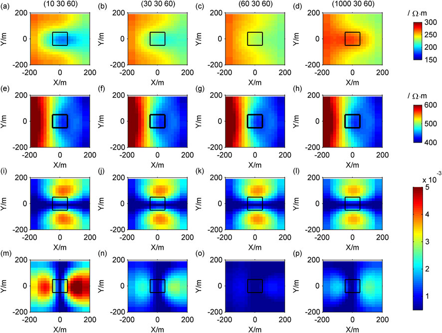
Figure 13. For non-plane waves, the contour maps of response of different resistivity in the X direction: (A–D)
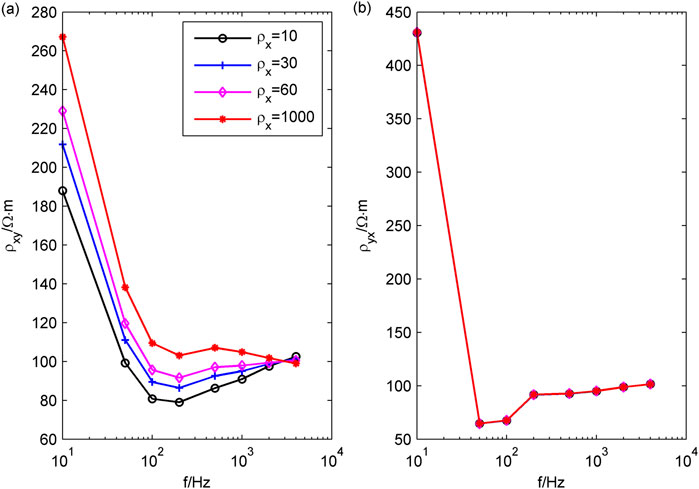
Figure 14. The curve of Cagniard resistivity with frequency at the center point of the receiving region when the resistivity changes in the X direction. (A)
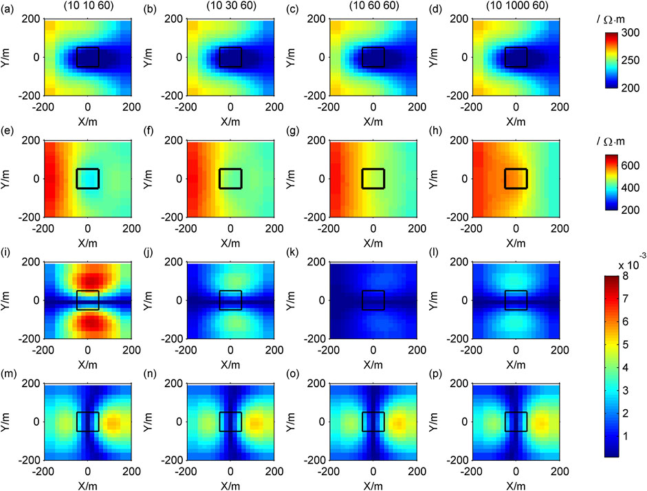
Figure 15. For non-plane waves, the contour maps of response of different resistivity in the Y direction: (A–D)
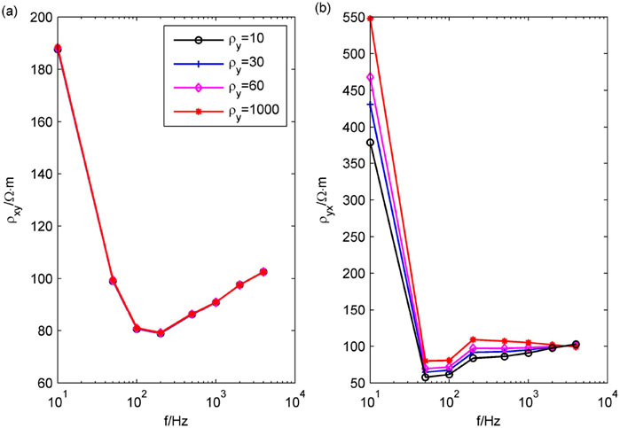
Figure 16. The curve of Cagniard resistivity with frequency at the center point of the receiving region when the resistivity changes in the Y direction. (A)
Compared with the response of plane waves (Figures 5A–D), the Cagniard resistivity
The
Whether it is an isotropic medium or an anisotropic medium, the CSAMT apparent resistivity in the near region will be distorted and needs to be corrected.
4 Conclusion
This study utilizes the 3D finite difference method to perform tensor CSAMT forward modeling in axis anisotropic media. The correctness of the algorithm is validated by comparing the results with Key’s 2D finite element algorithm. The forward modeling examples demonstrate that Cagniard resistivity exhibits low-value anomalies for low-resistance bodies and high-value anomalies for high-resistance bodies. Tippers are capable of reflecting the horizontal boundaries of anomalous bodies. The resistivity changes of the anomalous body are found to have different sensitivities in the X and Y directions, influenced by the polarization direction of the electric field. Specifically,
In the near region, the CSAMT signal of non-plane waves induces distortion in the Cagniard resistivity. The characteristics of tippers for non-plane waves are similar to those of plane waves. When exploring anisotropic media, tensor CSAMT proves advantageous in identifying changes in resistivity in two-axis (X and Y) directions compared to scalar CSAMT.
Whether utilizing the MT method (Kong et al., 2023) or the CSAMT method, the Cagniard resistivity and tipper demonstrate poor sensitivity to resistivity changes in the Z direction. Therefore, investigating methods to improve the identification of anisotropic Z direction (vertical) resistivity using electromagnetic techniques is a topic worthy of further study.
Data availability statement
The raw data supporting the conclusions of this article will be made available by the authors, without undue reservation.
Author contributions
XL: Conceptualization, Data curation, Formal Analysis, Funding acquisition, Investigation, Methodology, Project administration, Resources, Software, Validation, Visualization, Writing–original draft, Writing–review and editing. SG: Conceptualization, Supervision, Validation, Writing–review and editing.
Funding
The author(s) declare that financial support was received for the research, authorship, and/or publication of this article. This work is funded financially by Heilongjiang Province Basic Research Business Expenses for Universities Heilongjiang University Special Fund Project (Grant No. 2023-KYYWF-1494) and the Natural Science Foundation of Jiangxi Province (Grant No. 20212BAB213023).
Acknowledgments
Thank you to the reviewers for their valuable feedback on this article, Professor Siripunvaraporn, Xie Maobi, and others for their previous research work, and the editor for their enthusiastic assistance. Thank you to Wenxin Kong for his enthusiastic help.
Conflict of interest
The authors declare that the research was conducted in the absence of any commercial or financial relationships that could be construed as a potential conflict of interest.
Publisher’s note
All claims expressed in this article are solely those of the authors and do not necessarily represent those of their affiliated organizations, or those of the publisher, the editors and the reviewers. Any product that may be evaluated in this article, or claim that may be made by its manufacturer, is not guaranteed or endorsed by the publisher.
References
Boerner, D. E., Wright, J. A., Thurlow, J. G., and Reed, L. E. (1993). Tensor CSAMT studies at the buchans mine in central newfoundland. Geophysics 58 (1), 12–19. doi:10.1190/1.1443342
Cai, H. Z., Xiong, B., and Michael, Z. (2015). Three-dimensional marine controlled-source electromagnetic modelling in anisotropic medium using finite element method. Chin. J. Geophys. 58 (08), 2839–2850. doi:10.6038/cjg20150818
Caldwell, G. T., Bibby, M. H., and Brown, C. (2002). Controlled source apparent resistivity tensors and their relationship to the magnetotelluric impedance tensor. Geophys. J. Int. 151 (3), 755–770. doi:10.1046/j.1365-246X.2002.01798.x
Cao, H., Wang, K. P., Wang, X. B., Duan, C. S., Lan, X., Luo, W., et al. (2021). Tipper data forward modeling and inversion of three-dimensional tensor CSAMT. J. Appl. Geophys. 193, 104432–104441. doi:10.1016/j.jappgeo.2021.104432
Chen, X. Z., Liu, Y. H., Yin, C. C., Qiu, C. K., Zhang, J., Ren, X. Y., et al. (2020). Three-dimensional inversion of controlled-source audio-frequency magnetotelluric data based on unstructured finite-element method. Appl. Geophys. 17 (3), 349–360. doi:10.1007/s11770-020-0812-z
Di, Q. Y., Fu, C. M., An, Z. G., Wang, R., Wang, G. J., Wang, M. Y., et al. (2020). An application of CSAMT for detecting weak geological structures near the deeply buried long tunnel of the shijiazhuang-taiyuan passenger railway line in the taihang mountains. Eng. Geol. 268 (1), 105517. doi:10.1016/j.enggeo.2020.105517
Garcia, X., Boerner, D., and Pedersen, L. B. (2003). Electric and magnetic galvanic distortion decomposition of tensor CSAMT data. Application to data from the Buchans Mine (Newfoundland, Canada). Geophys. J. Int. 154 (3), 957–969. doi:10.1046/j.1365-246X.2003.02019.x
Guo, Z. W., Hu, L. T., Liu, C. M., Cao, C. H., Liu, J. X., and Liu, R. (2019). Application of the CSAMT method to Pb–Zn mineral deposits: a case study in jianshui, China. Minerals 9 (12), 726. doi:10.3390/min9120726
He, G. L., Xiao, T. J., Wang, Y., and Wang, G. J. (2019). 3D CSAMT modelling in anisotropic media using edge-based finite-element method. Explor. Geophys. 50 (1), 42–56. doi:10.1080/08123985.2019.1565914
Hui, Z. J. (2021) “3D forward modeling and inversion for time-domain marine CSEM based on unstructured finite element method,” in School of Earth exploration science and Technology. Changchun, China: Jilin University. PhD thesis.
Key, K. (2009). 1D inversion of multicomponent, multifrequency marine CSEM data: Methodology and synthetic studies for resolving thin resistive layers. Geophysics 74 (2), F9–F20. doi:10.1190/1.3058434
Key, K. (2016). MARE2DEM: a 2-D inversion code for controlled-source electromagnetic and magnetotelluric data. Geophys. J. Int. 207 (1), 571–588. doi:10.1093/gji/ggw290
Kirkby, A., Heinson, G., Holford, S., and Thiel, S. (2015). Mapping fractures using 1D anisotropic modelling of magnetotelluric data: a case study from the Otway Basin, Victoria, Australia. Geophys. J. Int. 201 (3), 1961–1976. doi:10.1093/gji/ggv116
Kong, W. X., Yu, N., Li, X., Zhang, X. J., Chen, H., Li, T. Y., et al. (2023). Three-dimensional axially anisotropic inversion of magnetotelluric phase tensor and tipper data. Chin. J. Geophys. 66 (9), 3928–3946. doi:10.6038/cjg2023R0040
Li, X. B., and Pedersen, L. B. (1991). Controlled-source tensor magnetotelluric responses of a layered earth with azimuthal anisotropy. Geophys. J. Int. 111 (1), 91–103. doi:10.1111/j.1365-246X.1992.tb00557.x
Li, Y., Wu, X. P., Lin, P. R., Han, S. X., Li, D., and Liu, W. D. (2017). Three-dimensional modeling of marine controlled-source electromagnetism using the vector finite element method for arbitrary anisotropic media. Chin. J. Geophys. 60 (5), 1955–1978. doi:10.6038/cjg20170528
Li, Y. G., and Key, K. (2007). 2D marine controlled-source electromagnetic modeling: Part 1 — an adaptive finite-element algorithm. Geophysics 72 (2), WA51–WA62. doi:10.1190/1.2432262
Liu, X., and Sun, Q.Ji (2024). A study of 3D axis anisotropic response of MT. Front. Earth Sci. 12, 1454962. doi:10.3389/feart.2024.1454962
Liu, X., Wang, M., and Chen, B. (2021). 3D tensor CSAMT modeling based on axis anisotropic media. Chin. J. Prog. Geophys. 36 (3), 1095–1102. doi:10.6038/pg2021EE0237
Liu, X., and Zheng, F. W. (2024). Axis anisotropic Occam’s 3D inversion of tensor CSAMT in data space. Appl. Geophys. doi:10.1007/s11770-024-1076-9
Liu, Y. H., Yin, C. C., Cai, J., Huang, W., Ben, F., Zhang, B., et al. (2018). Review on research of electrical anisotropy in electromagnetic prospecting. Chin. J. Geophys. 61 (8), 3468–3487. doi:10.6038/cjg2018L0004
Qiu, C. K., Yin, C. C., Liu, Y. H., Chen, H., Liu, L., and Cai, J. (2018). 3D forward modeling of controlled-source audio-frequency magnetotellurics in arbitrarily anisotropic media. Chin. J. Geophys. 61 (8), 3488–3498. doi:10.6038/cjg2018L0326
Siripunvaraporna, W., Egbertb, G., and Lenbury, Y. (2002). Numerical accuracy of magnetotelluric modeling: a comparison of finite difference approximations. Earth Planets Space 54, 721–725. doi:10.1186/BF03351724
Wang, G., Lei, D., Zhang, Z. Y., Hu, X. Y., Li, Y. B., Wang, D. Y., et al. (2018a). Tensor CSAMT and AMT studies of the Xiarihamu Ni-Cu sulfide deposit in Qinghai, China. J. Appl. Geophys. 159, 795–802. doi:10.1016/j.jappgeo.2018.09.031
Wang, K. P., and Tan, H. D. (2017). Research on the forward modeling of controlled-source audio-frequency magnetotellurics in three-dimensional axial anisotropic media. J. Appl. Geophys. 146, 27–36. doi:10.1016/j.jappgeo.2017.08.007
Wang, K. P., Tan, H. D., Lin, C. H., Yuan, J. L., Wang, C., and Tang, J. (2018b). Three-dimensional tensor controlled-source audio-frequency magnetotelluric inversion using LBFGS. Explor. Geophys. 49 (3), 268–284. doi:10.1071/EG16079
Wang, T., Wang, K. P., and Tan, H. D. (2017). Forward modeling and inversion of tensor CSAMT in 3D anisotropic media. Appl. Geophys. 14 (04), 590–605. doi:10.1007/s11770-017-0644-7
Xie, M. B., Tan, H. D., Wang, K. P., Guo, C. A., Zhang, Z. Y., and Li, Z. Q. (2016). Study on the characteristics of 3D CSAMT tensor impedance data. Chin. J. Prog. Geophys. 32 (2), 0522–0530. doi:10.6038/pg20170210
Xu, Z. M., Tang, J. T., Li, G., Xin, H. C., Xu, Z. J., Tan, X. P., et al. (2020). Groundwater resources survey of tongchuan city using the audio magnetotelluric method. Appl. Geophys. 17 (5-6), 660–671. doi:10.1007/s11770-018-0709-2
Xue, G. Q., Yan, S., Gelius, L. J., Chen, W. Y., Zhou, N. N., and Li, H. (2015). Discovery of a major coal deposit in China with the use of a modified CSAMT method. J. Environ. and Eng. Geophys. 20 (1), 47–56. doi:10.2113/JEEG20.1.47
Keywords: tensor CSAMT, axis anisotropy, Cagniard resistivity, tipper, forward algorithm
Citation: Liu X and Gao S (2024) Response characteristics of 3D tensor CSAMT in axis anisotropic media. Front. Earth Sci. 12:1449515. doi: 10.3389/feart.2024.1449515
Received: 15 June 2024; Accepted: 24 September 2024;
Published: 11 October 2024.
Edited by:
Bo Zhang, Jilin University, ChinaReviewed by:
Xiaoyue Cao, Key Laboratory of Exploration Technologies for Oil and Gas Resource (Yangtze University), ChinaCong Zhou, East China University of Technology, China
Rong Liu, Central South University, China
Copyright © 2024 Liu and Gao. This is an open-access article distributed under the terms of the Creative Commons Attribution License (CC BY). The use, distribution or reproduction in other forums is permitted, provided the original author(s) and the copyright owner(s) are credited and that the original publication in this journal is cited, in accordance with accepted academic practice. No use, distribution or reproduction is permitted which does not comply with these terms.
*Correspondence: Shijie Gao, Z3NqQGVtYWlsLmN1Z2IuZWR1LmNu