A study of 3D axis anisotropic response of MT

Electrical anisotropy has a significant impact on the observation data of the magnetotelluric (MT) method; therefore, it is necessary to develop forward and inverse methods in electrical anisotropic media. Based on the axis anisotropic electric field control equations, forming a large linear equation through staggered finite difference approximation, adding boundary conditions, and using the quasi-minimum residual method to solve the equation, this study obtained MT forward modeling results in axis anisotropic media. The correctness of the algorithm was verified by comparing it with the 2D quasi-analytic solution. By designing several sets of axis anisotropic 3D models, the characteristics of the apparent resistivity tensor and tipper were analyzed. The results indicated that the ${\rho }_{xy}^a$, ${\rho }_{yy}^a$ and $T_{zy}$ are sensitive to changes in resistivity in the X direction of the anomalous body, whereas the ${\rho }_{yx}^a$, ${\rho }_{xx}^a$ and $T_{zx}$ are sensitive to changes in resistivity in the Y direction. The apparent resistivity tensor and tipper are insensitive to changes in resistivity in the Z direction of the anomalous body. For exploration of anisotropic media, the apparent resistivity tensor and tipper of MT can identify the changes in resistivity in two horizontal axes directions and the boundaries of the anomalous body, which has the advantages for exploration.

1 Introduction

Anisotropy is commonly present in the crust and upper mantle. Fractures and rock bedding in certain specific directions, as well as the stacking combination of uniform thin layers with different properties, can cause electrical anisotropy in the lithospheric structure (Postma, 1955; Wannamaker, 2005). The practice and research of geophysical exploration have shown that electrical anisotropy has a significant impact on electromagnetic observation data and that directly using isotropic models to fit data containing electrical anisotropy can result in significant errors (Yin and Weidelt, 1999; Liu and Zheng, 2024). Therefore, to improve the accuracy of electromagnetic inversion results, including magnetotelluric methods, and the level of understanding of underground structures, it is necessary to develop electromagnetic data processing and inversion methods based on anisotropic models (Liu Y. H. et al., 2018).

Research on magnetotelluric anisotropy has been increasing (Qin et al., 2022). Based on 2D numerical forward modeling techniques (Pek and Verner, 1997; Li, 2002), 3D forward modeling research results, especially the finite volume method (Han et al., 2018), the finite element method (Cao et al., 2018; Xiao et al., 2018; Liu Y. et al, 2018; Guo et al., 2020; Ye et al., 2021; Zhou et al., 2021) and the finite difference method (Yu et al., 2018; Kong, 2021), continue to emerge. The finite element method has strong simulation ability for complex shapes and terrains, and it establishes variational equations through the Galerkin method. A weighted posterior error estimation method was constructed using the continuity condition of current density, which has been used to calculate the magnetotelluric (MT) response of arbitrary anisotropic media (Cao et al., 2018). The finite difference method ensures that the distribution of the electromagnetic field satisfies the law of energy conservation and also simplifies the derivation of the equations.

Because of the complexity of numerical simulation for arbitrary anisotropy, this study considers the case of axis anisotropy. Axis anisotropy can be understood as the difference in conductivity in the three directions of the medium caused by factors such as mineral orientation. The conductivity tensor of arbitrary anisotropy can be obtained by three Euler rotations of the axis anisotropy. Kong (2021) used direct discretization of Maxwell’s equations to achieve MT anisotropic forward modeling. In this study, the electric field control equation is solved to achieve MT axis anisotropic forward modeling. The algorithm is implemented by Fortran program. The response characteristics of the axis anisotropic target body are analyzed through three numerical examples, providing a basis for conducting MT forward and reverse modeling research with arbitrary anisotropy.

2 MT 3D forword modeling method

2.1 Finite difference method for calculating MT fields

For isotropic media, ignoring displacement current, the frequency domain control equation of the magnetotelluric method is

$\nabla \times \mathbf{E}=i\omega {\mu }_0\mathbf{H}(1)$

$\nabla \times \mathbf{H}=\sigma \mathbf{E}(2)$

where $\nabla$ represents the Nabla operator, $\mathbf{E}$ represents the electric field, $i$ represents an imaginary unit, $\omega$ represents the angular frequency, ${\mu }_0$ represents the vacuum magnetic permeability, $\mathbf{H}$ represents the magnetic field, and $\sigma$ represents the conductivity.

After organizing Equations 1, 2, the following electric field control equation is obtained:

$\nabla \times \nabla \times \mathbf{E}=i\omega {\mu }_0\sigma \mathbf{E}(3)$

For 3D axis anisotropic medial, the tensor conductivity is

$\mathbf{\sigma }=\left(\begin{array}{l}{\sigma }_{x}00\\ 0{\sigma }_{y}0\\ 00{\sigma }_z\end{array}\right)(4)$

By substituting Equation 4 into Equation 3 and organizing, the following equations can be obtained:

$\frac{\partial }{\partial y}\left[\frac{\partial E_y}{\partial x}-\frac{\partial E_x}{\partial y}\right]-\frac{\partial }{\partial z}\left[\frac{\partial E_x}{\partial z}-\frac{\partial E_z}{\partial x}\right]=\omega {\mu }_0{\sigma }_x{E}_x(5)$

$\frac{\partial }{\partial z}\left[\frac{\partial E_z}{\partial y}-\frac{\partial E_y}{\partial z}\right]-\frac{\partial }{\partial x}\left[\frac{\partial E_y}{\partial x}-\frac{\partial E_x}{\partial y}\right]=i\omega {\mu }_0{\sigma }_y{E}_y(6)$

$\frac{\partial }{\partial x}\left[\frac{\partial E_x}{\partial z}-\frac{\partial E_y}{\partial x}\right]-\frac{\partial }{\partial y}\left[\frac{\partial E_z}{\partial y}-\frac{\partial E_y}{\partial z}\right]=i\omega {\mu }_0{\sigma }_z{E}_z(7)$

Using the staggered finite difference approximation Equations 5–7, the following equation is obtained after sorting (Siripunvaraporna et al., 2005):

$\mathbf{A}\mathbf{X}=\mathbf{b}(8)$

where $\mathbf{A}$ is a symmetric large sparse coefficient matrix, $\mathbf{X}$ is a vector composed of three components of the electric field at the sampling point, and $\mathbf{b}$ is a vector composed of boundary electric field components.

When a sufficiently thick air layer is added, the influence of anomalous bodies on the top boundary of the air layer can be ignored. The four lateral boundaries can be regarded as 2D geoelectric interfaces, solved using 2D MT anisotropic finite difference codes (Kong, 2021). After introducing the boundary conditions, the three component values of the electric field in the partitioned space are obtained by solving Equation 8 using the quasi-minimum residual (QMR) method, with a preconditioner formed by an incomplete LU decomposition (Siripunvaraporna et al., 2002). To accelerate the convergence of QMR iteration, divergence correction (Smith, 1996) is also applied to the solution of the electric field. The electric and magnetic field components of each measurement point on the surface are obtained through electric field interpolation.

2.2 Calculating tensor impedance and tipper

Calculate the magnetotelluric response using TE and TM polarization simulations, denoted as $E_{x1}$, $E_{y1}$, $H_{x1}$, $H_{y1}$ and $H_{z1}$, $E_{x2}$, $E_{y2}$, $H_{x2}$, $H_{y2}$ and $H_{z2}$. So the expressions for the magnetotelluric impedance component and tipper component are obtained:

$\begin{array}{l}{Z}_{xx}=\frac{E_{x1}{H}_{y2}-E_{x2}{H}_{y1}}{H_{x1}{H}_{y2}-H_{x2}{H}_{y1}},Z_{xy}=\frac{E_{x2}{H}_{y1}-E_{x1}{H}_{x2}}{H_{x1}{H}_{y2}-H_{x2}{H}_{y1}}\\ Z_{yx}=\frac{E_{y1}{H}_{y2}-E_{y2}{H}_{y1}}{H_{x1}{H}_{y2}-H_{x2}{H}_{y1}},Z_{yy}=\frac{E_{y2}{H}_{x1}-E_{y1}{H}_{x2}}{H_{x1}{H}_{y2}-H_{x2}{H}_{y1}}\end{array}(9)$

$T_{zx}=\frac{H_{z1}{H}_{y2}-H_{z2}{H}_{y1}}{H_{x1}{H}_{y2}-H_{x2}{H}_{y1}},T_{zy}=\frac{H_{z2}{H}_{x1}-H_{z1}{H}_{x2}}{H_{x1}{H}_{y2}-H_{x2}{H}_{y1}}(10)$

The corresponding apparent resistivity tensor and apparent phase tensor are:

$\begin{array}{l}{\rho }_{ij}^a=\frac{1}{\omega {\mu }_0}{\left|Z_{ij}\right|}^2\\ {\varphi }_{ij}={\tan }^{-1}\left(\text{Im}\left(Z_{ij}\right)/\text{Re}\left(Z_{ij}\right)\right)\end{array}(11)$

where $i=x,y$, $j=x,y$. In the following text, the axial anisotropy response of MT is calculated by Equations 9–11.

2.3 Algorithm validation

To verify the correctness of the algorithm, we compared it with the quasi-analytic solution of Qin et al. (2013), who established a 2D axis anisotropic upright fault model (Figure 1). The left side of the fault is an axis anisotropic block, with resistivity values of 10, 100, and 10 $\mathrm{\Omega }·m$ in the X, Y, and Z directions, respectively. The right side of the fault is an isotropic block, with resistivity values of 1,000 $\mathrm{\Omega }·m$. A frequency of 0.1 Hz is used.

Figure 1

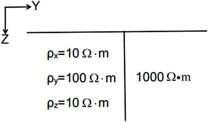
Figure 1. Sketch of the 2D axis anisotropic model.

In TM mode, the comparison results of apparent resistivity and apparent phase and curve of relative residual error of the QMR iteration are shown in Figure 2. The 3D finite difference results and 2D quasi-analytic solution fit well, with only a slight error at the fault interface (Figures 2A–D), indicating that the calculation results of the forward program are correct. The QMR iteration converges stably to the given tolerance (Figure 2E).

Figure 2

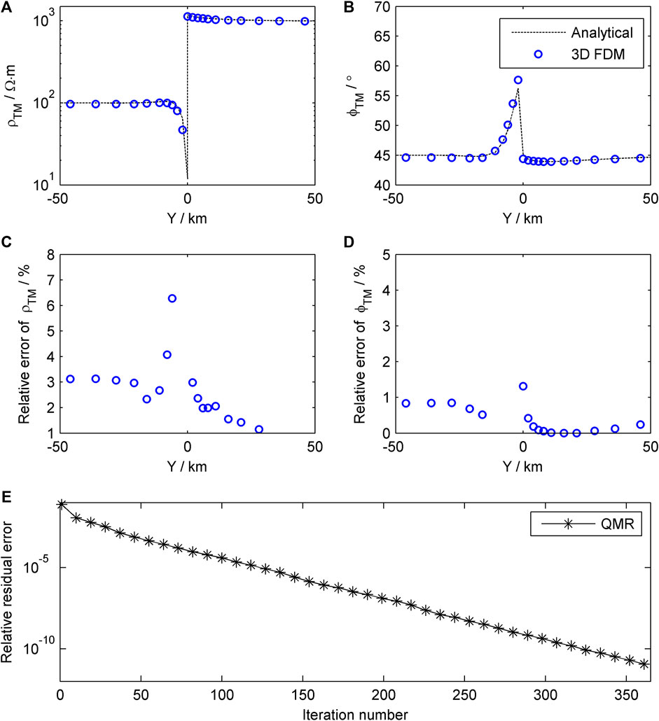
Figure 2. Comparison of the results of 3D forward modeling and 2D quasi-analytic solution (A–D) and curve of relative residual error of the QMR iteration (E).

3 3D axis anisotropic forward modeling case of MT

3.1 Response of 3D axis anisotropic low-resistance prism

The 3D prism model is shown in Figure 3. The top surface of the prism is buried at a depth of 100 m, and the prism has a size of 8 km × 8 km × 5 km. The background resistivity is 100 $\mathrm{\Omega }·m$, and the mesh size is 28 × 28 × 28, which includes 7 air layers. The frequency of the MT used is 10 Hz.

Figure 3

Figure 3. Sketch of the 3D axis anisotropic low-resistance model.

To study the impact of the axis anisotropy of low-resistance bodies on MT forward modeling, we designed several sets of examples. We first fix the resistivity of the low-resistance body in the Y and Z directions (${\rho }_y=30\mathrm{\Omega }\cdot m$ and ${\rho }_z=60\mathrm{\Omega }\cdot m$), with resistivity in the X-direction of 10, 30, and 90 $\mathrm{\Omega }·m$, respectively, and apply the algorithm proposed in this study for forward modeling. The resulting surface contour map is shown in Figure 4. Next, we fix the resistivity of the low-resistance body in the X and Z directions (${\rho }_x=30\mathrm{\Omega }\cdot m$ and ${\rho }_z=60\mathrm{\Omega }\cdot m$), with resistivity in the Y-direction of 10, 30, and 90 $\mathrm{\Omega }·m$, respectively. These forward results are shown in Figure 5. Finally, we fix the resistivity of the low-resistance body in the X and Y directions (${\rho }_x=30\mathrm{\Omega }\cdot m$ and ${\rho }_y=60\mathrm{\Omega }\cdot m$), with the resistivity in the Z-direction of 10, 30, and 90 $\mathrm{\Omega }·m$, respectively. The forward results for this example are shown in Figure 6.

Figure 4

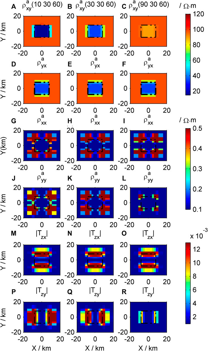
Figure 4. Contour maps of the response of the different low-resistivity models in the X direction: (A–C) ${\rho }_{xy}^a$; (D–F) ${\rho }_{yx}^a$; (G–I) ${\rho }_{xx}^a$; (J–L) ${\rho }_{yy}^a$; (M–O) $\left|T_{zx}\right|$; (P–R) $\left|T_{zy}\right|$.

Figure 5

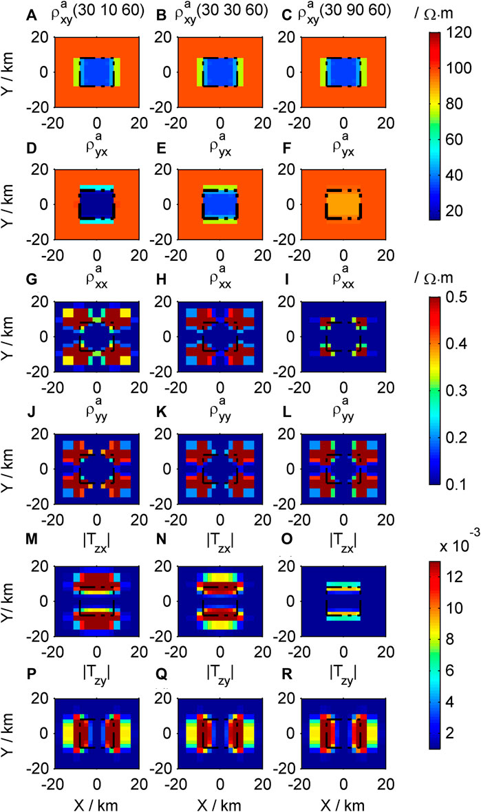
Figure 5. Contour maps of the response of the different low-resistivity models in the Y direction: (A–C) ${\rho }_{xy}^a$; (D–F) ${\rho }_{yx}^a$; (G–I) ${\rho }_{xx}^a$; (J–L) ${\rho }_{yy}^a$; (M–O) $\left|T_{zx}\right|$; (P–R) $\left|T_{zy}\right|$.

Figure 6

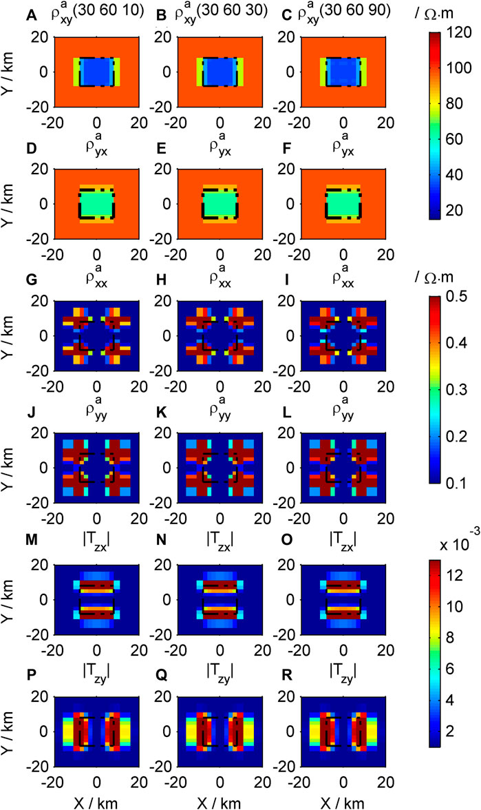
Figure 6. Contour maps of the response of the different low-resistivity models in the Z direction: (A–C) ${\rho }_{xy}^a$; (D–F) ${\rho }_{yx}^a$; (G–I) ${\rho }_{xx}^a$; (J–L) ${\rho }_{yy}^a$; (M–O) $\left|T_{zx}\right|$; (P–R) $\left|T_{zy}\right|$.

The apparent resistivity ${\rho }_{xy}^a$ and ${\rho }_{yx}^a$ reflects the horizontal position of the low-resistance body, and the apparent resistivity ${\rho }_{xx}^a$, ${\rho }_{yy}^a$, and the tipper $T_{zx}$, $T_{zy}$ clearly reflect the horizontal boundary of the low-resistance body (Figure 4). The amplitudes of ${\rho }_{yy}^a$ and ${\rho }_{yx}^a$ are much greater than those of ${\rho }_{xx}^a$ and ${\rho }_{yy}^a$ (Figures 4A–L). ${\rho }_{xy}^a$, ${\rho }_{yy}^a$, and $T_{zy}$ are sensitive to changes in resistivity in the X direction (${\rho }_x$) of the low-resistance body. When the resistivity of the low-resistance body is lower, the anomalies it produces are more obvious (Figures 4A–C, J–L, P–R). ${\rho }_{yx}^a$, ${\rho }_{xx}^a$, and $T_{zx}$ are insensitive to changes in resistivity in the X direction of the low-resistance body (Figures 4D–I, M–O), and are less affected by the resistivity in the X-direction.

${\rho }_{xy}^a$, ${\rho }_{yy}^a$, and $T_{zy}$ are insensitive to changes in resistivity in the Y direction (${\rho }_y$) of the low-resistance body, and are less affected by the resistivity in the Y direction (Figures 5A–C, J–L, P–R). ${\rho }_{yx}^a$, ${\rho }_{xx}^a$, and $T_{zx}$ are sensitive to changes in resistivity in the Y-direction of the low-resistance body. As the resistivity of the low-resistance body becomes lower, the anomalies it produces become more obvious (Figures 5D–I, M–O).

The impacts of resistivity changes in the X and Y directions of the low-resistance body on response results are different.

The apparent resistivity tensor and tipper are not sensitive to changes in resistivity in the Z direction of the low resistivity body (Figures 6A–R), indicating that ${\rho }_z$ has a weak contribution to the surface response. For MT, in TE mode, the polarization direction of the electric field is mainly in the X direction, therefore it is sensitive to changes in resistivity in the X direction; in TM mode, the polarization direction of the electric field is mainly in the Y direction, therefore it is sensitive to changes in resistivity in the Y direction (Wang et al., 2017).

A contour map of apparent resistivity based on the relationship between apparent resistivity and frequency is shown in Figure 7. The low-value anomaly areas of apparent resistivity ${\rho }_{xy}^a$ and ${\rho }_{yx}^a$ are not closed. As the detection depth of MT increases with decreasing frequency, the relatively low-value anomaly areas are equivalent to extending deeper underground (Figure 7).

Figure 7

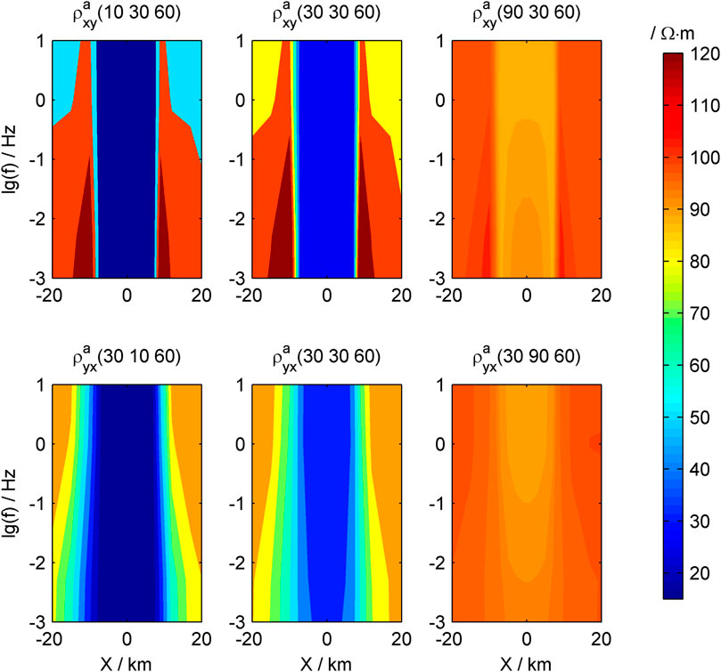
Figure 7. Pseudo-contour maps of the apparent resistivity of the low-resistivity body.

3.2 Response of 3D axis anisotropic high-resistance prism

The 3D prism model is the same as 3.1, except that the resistivity is set to high-resistance. The frequency of the MT used is 10 Hz.

We first fix ${\rho }_y=500\mathrm{\Omega }\cdot m$, ${\rho }_z=200\mathrm{\Omega }\cdot m$, with ${\rho }_x$ of 200, 500, and 1,000 $\mathrm{\Omega }·m$, respectively. The forward results are shown in Figure 8. Next, we fix ${\rho }_x=200\mathrm{\Omega }\cdot m$, ${\rho }_z=500\mathrm{\Omega }\cdot m$, with ${\rho }_y$ of 200, 500, and 1,000 $\mathrm{\Omega }·m$, respectively. The forward results are shown in Figure 9.

Figure 8

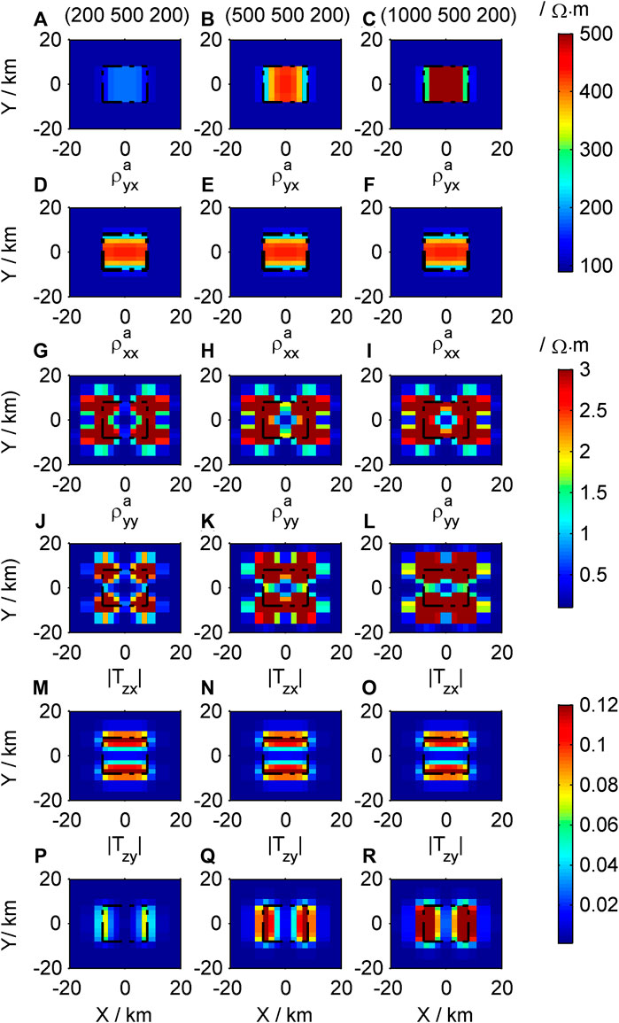
Figure 8. Contour maps of response of the different high-resistivity models in the X direction: (A–C) ${\rho }_{xy}^a$; (D–F) ${\rho }_{yx}^a$; (G–I) ${\rho }_{xx}^a$; (J–L) ${\rho }_{yy}^a$; (M–O) $\left|T_{zx}\right|$; (P–R) $\left|T_{zy}\right|$.

Figure 9

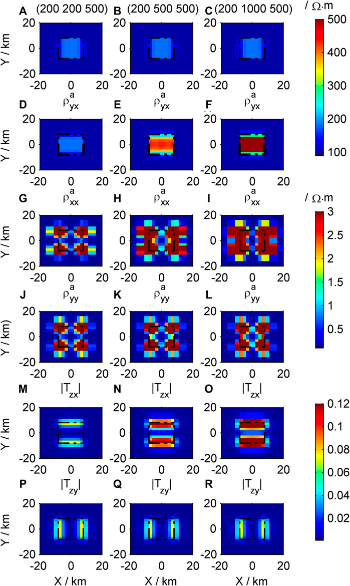
Figure 9. Contour maps of the response of different high-resistivity models in the Y direction: (A–C) ${\rho }_{xy}^a$; (D–F) ${\rho }_{yx}^a$; (G–I) ${\rho }_{xx}^a$; (J–L) ${\rho }_{yy}^a$; (M–O) $\left|T_{zx}\right|$; (P–R) $\left|T_{zy}\right|$.

The apparent resistivity ${\rho }_{xy}^a$ and ${\rho }_{yx}^a$ reflects the horizontal position of the high-resistance body, and the apparent resistivity ${\rho }_{xx}^a$, ${\rho }_{yy}^a$, and the tipper $T_{zx}$, $T_{zy}$ reflect the horizontal boundary of the high-resistance body (Figure 8). ${\rho }_{xy}^a$, ${\rho }_{yy}^a$, and $T_{zy}$ are sensitive to changes of ${\rho }_x$ of high-resistance body. When the resistivity of the high-resistance body is higher, the anomalies it produces are more obvious (Figures 8A–C, J–L, P–R). ${\rho }_{yx}^a$, ${\rho }_{xx}^a$, and $T_{zx}$ are less affected by the ${\rho }_x$ (Figures 8D–I, M–O).

The apparent resistivity ${\rho }_{xy}^a$, ${\rho }_{yy}^a$, and the tipper $T_{zy}$ are less affected by the ${\rho }_y$ of high-resistance body (Figures 9A–C, J–L, P–R). ${\rho }_{yx}^a$, ${\rho }_{xx}^a$, and $T_{zx}$ are sensitive to changes of ${\rho }_y$ of the high-resistance body and are greatly affected by it (Figures 9D–I, M–O). The apparent resistivity tensor and tipper are not sensitive to changes of ${\rho }_z$ of the high-resistivity body.

3.3 Response of 3D complex axis anisotropic prism

The plan view of the 3D complex prism model is shown in Figure 10. The top surface of the model is buried at a depth of 100 m, the size of the prisms on both sides is 5 km × 22 km × 5 km, and the main axis resistivity in the X, Y, and Z direction is 10, 1,000, and 100 $\mathrm{\Omega }\cdot m$, respectively. The total length and width of the middle prism are both 12 km, and the height is 5 km. The main axis resistivity in the X, Y, and Z direction is 30, 500, and 100 $\mathrm{\Omega }\cdot m$, respectively. The background resistivity is 100 $\mathrm{\Omega }\cdot m$, and the frequency of MT is 10 Hz. The forward modeling results are shown in Figure 11.

Figure 10

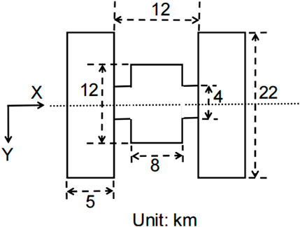
Figure 10. Plan view of the 3D complex model.

Figure 11

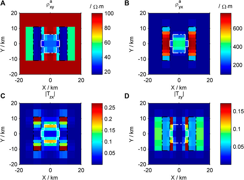
Figure 11. Contour maps of response of the 3D complex model.

Based on the previous analysis, according to Figure 11, the low-resistivity body in the X direction of the complex model caused the low value apparent resistivity anomaly zone of ${\rho }_{xy}^a$, and this anomaly zone reflects the boundary of the Y direction of the combination (Figure 11A). The high-resistivity anomaly zone of ${\rho }_{yx}^a$ is caused by the high resistivity body in the Y direction of the composite, and this anomaly zone clearly reflects the boundary of the composite in the X direction (Figure 11B). The anomalous regions of $T_{zx}$ and $T_{zy}$ respectively reflect the boundaries of the combination in the X and Y directions, respectively (Figures 11C, D).

4 Conclusion

This study applies the finite difference method to achieve 3D MT forward modeling in axis anisotropic media and verifies the correctness of the algorithm by comparing it with 2D quasi-analytic solution. The examples show that ${\rho }_{xy}^a$, ${\rho }_{yy}^a$, and $T_{zy}$ are sensitive to changes of ${\rho }_x$ of the anomalous body and are greatly affected by it, but insensitive to changes of ${\rho }_y$. ${\rho }_{yx}^a$, ${\rho }_{xx}^a$, and $T_{zx}$ are sensitive to changes of ${\rho }_y$ of the anomalous body and are greatly affected by it, but insensitive to changes of ${\rho }_x$. The apparent resistivity tensor and tipper are not sensitive to changes of ${\rho }_z$ of the anomalous body. ${\rho }_z$ has a weak contribution to the surface response of MT. For the exploration of anisotropic media, the apparent resistivity tensor and tipper can identify the changes in resistivity in two horizontal axes directions and the boundaries of the anomalous body, which has the advantage for exploration. The study provides a basis for conducting the forward modeling and inversion research of MT with arbitrary anisotropy.

Data availability statement

The original contributions presented in the study are included in the article/supplementary material, further inquiries can be directed to the corresponding author.

Author contributions

XL: Conceptualization, Data curation, Formal Analysis, Funding acquisition, Investigation, Methodology, Project administration, Resources, Software, Supervision, Validation, Visualization, Writing–original draft, Writing–review and editing. Q-JS: Methodology, Validation, Writing–review and editing.

Funding

The author(s) declare that financial support was received for the research, authorship, and/or publication of this article. This work is funded financially by Heilongjiang Province Basic Research Business Expenses for Universities Heilongjiang University Special Fund Project (Grant No. 2023-KYYWF-1494) and the Natural Science Foundation of Jiangxi Province (Grant No. 20212BAB213023).

Acknowledgments

Thank you to the reviewers for their valuable feedback on this article, Professor Siripunvaraporn, and others for their previous research work, and the editor for their enthusiastic assistance. Thank you to Wenxin Kong for his enthusiastic help. We would like to thank Editage (www.editage.cn) for English language editing.

Conflict of interest

The authors declare that the research was conducted in the absence of any commercial or financial relationships that could be construed as a potential conflict of interest.

Publisher’s note

All claims expressed in this article are solely those of the authors and do not necessarily represent those of their affiliated organizations, or those of the publisher, the editors and the reviewers. Any product that may be evaluated in this article, or claim that may be made by its manufacturer, is not guaranteed or endorsed by the publisher.

References

Cao, X. Y., Yin, C. C., Zhang, B., Huang, X., Liu, Y. H., and Cai, J. (2018). A goal-oriented adaptive finite-element method for 3D MT anisotropic modeling with topography. Chin. J. Geophys. 61 (6), 2618–2628. doi:10.6038/cjg2018L0068

CrossRef Full Text | Google Scholar

Guo, Z. Q., Egbert, G., Dong, H., and Wei, W. (2020). Modular finite volume approach for 3D magnetotelluric modeling of the Earth medium with general anisotropy. Phys. Earth Planet. Interiors 309, 106585. doi:10.1016/j.pepi.2020.106585

CrossRef Full Text | Google Scholar

Han, B., Li, Y. G., and Li, G. (2018). 3D forward modeling of magnetotelluric fields in general anisotropic media and its numerical implementation in Julia. Geophysics 83 (4), F29–F40. doi:10.1190/GEO2017-0515.1

CrossRef Full Text | Google Scholar

Kong, W. X. (2021). Research on the three-dimensional anisot ropic inversion of magnetotelluric data. Ph. D. thesis. Beijing: China University of Geosciences.

Google Scholar

Li, Y. G. (2002). A finite-element algorithm for electromagnetic induction in two-dimensional anisotropic conductivity structures. Geophys. J. Int. 148 (3), 389–401. doi:10.1046/j.1365-246x.2002.01570.x

CrossRef Full Text | Google Scholar

Liu, X., and Zheng, F. W. (2024). Axis anisotropic Occam’s 3D inversion of tensor CSAMT in data space. Appl. Geophys. doi:10.1007/s11770-024-1076-9

CrossRef Full Text | Google Scholar

Liu, Y., Xu, Z. H., and Li, Y. G. (2018). Adaptive finite element modelling of three-dimensional magnetotelluric fields in general anisotropic media. J. Appl. Geophys. 151, 113–124. doi:10.1016/j.jappgeo.2018.01.012

CrossRef Full Text | Google Scholar

Liu, Y. H., Yin, C. C., Cai, J., Huang, W., Ben, F., Zhang, B., et al. (2018). Review on research of electrical anisotropy in electromagnetic prospecting. Chin. J. Geophys. 61 (8), 3468–3487. doi:10.6038/cjg2018L0004

CrossRef Full Text | Google Scholar

Pek, J., and Verner, T. (1997). Finite -difference modelling of magnetotelluric fields in two dimensional anisotropic media. Geophys. J. Int. 128 (3), 505–521. doi:10.1111/j.1365-246X.1997.tb05314.x

CrossRef Full Text | Google Scholar

Postma, G. W. (1955). Wave propagation in a stratified medium. Geophysics 20 (4), 780–806. doi:10.1190/1.1438187

CrossRef Full Text | Google Scholar

Qin, L. J., Ding, W. F., and Yang, C. F. (2022). Magnetotelluric responses of an anisotropic 1-D earth with a layer of exponentially varying conductivity. Minerals 12 (7), 915. doi:10.3390/min12070915

CrossRef Full Text | Google Scholar

Qin, L. J., Yang, C. F., and Chen, K. (2013). Quasi analytic solution of 2-D magnetotelluric fields on an axially anisotropic infinite fault. Geophys. J. Int. 192 (1), 67–74. doi:10.1093/gji/ggs018

CrossRef Full Text | Google Scholar

Siripunvaraporna, W., Egbertb, G., and Lenbury, Y. (2002). Numerical accuracy of magnetotelluric modeling: a comparison of finite difference approximations. Earth Planets Space 54, 721–725. doi:10.1186/BF03351724

CrossRef Full Text | Google Scholar

Siripunvaraporna, W., Egbertb, G., Lenbury, Y., and Uyeshima, M. (2005). Three-dimensional magnetotelluric inversion: data-space method. Phys. Earth Planet. Interiors 150 (1–3), 3–14. doi:10.1016/j.pepi.2004.08.023

CrossRef Full Text | Google Scholar

Smith, J. T. (1996). Conservative modeling of 3D electromagnetic fields. Part II. Biconjugate gradient solution and an accelerator. Geophysics 61 (5), 1319–1324. doi:10.1190/1.1444055

CrossRef Full Text | Google Scholar

Wang, T., Wang, K. P., and Tan, H. D. (2017). Forward modeling and inversion of tensor CSAMT in 3D anisotropic media. Appl. Geophys. 14 (04), 590–605. doi:10.1007/s11770-017-0644-7

CrossRef Full Text | Google Scholar

Wannamaker, P. E. (2005). Anisotropy versus heterogeneity in continental solid earth electromagnetic studies: fundamental response characteristics and implications for physicochemical state. Surv. Geophys. 26 (6), 733–765. doi:10.1007/s10712-005-1832-1

CrossRef Full Text | Google Scholar

Xiao, T. J., Huang, X. Y., and Wang, Y. (2018). 3D MT modeling using the T-Ω method in general anisotropic media. J. Appl. Geophys. 160, 171–182. doi:10.1016/j.jappgeo.2018.11.012

CrossRef Full Text | Google Scholar

Ye, Y. X., Du, J. M., Liu, Y., Ai, A. M., and Jiang, F. Y. (2021). Three-dimensional magnetotelluric modeling in general anisotropic media using nodal-based unstructured finite element method. Comput and Geosciences 148, 104686. doi:10.1016/j.cageo.2021.104686

CrossRef Full Text | Google Scholar

Yin, C. C., and Weidelt, P. (1999). Geoelectrical fields in a layered earth with arbitrary anisotropy. Geophysics 64 (2), 426–434. doi:10.1190/1.1444547

CrossRef Full Text | Google Scholar

Yu, G., Xiao, Q. B., Zhao, G. Z., and Li, M. (2018). Three-dimensional magnetotelluric responses for arbitrary electrically anisotropic media and a practical application. Geophys. Prospect. 66 (9), 1764–1783. doi:10.1111/1365-2478.12690

CrossRef Full Text | Google Scholar

Zhou, J. J., Hu, X. Y., and Cai, H. Z. (2021). Three -dimensional finite-element analysis of magnetotelluric data using coulomb -gauged potentials in general anisotropic media. Pure Appl. Geophys. 178 (11), 4561–4581. doi:10.1007/s00024-021-02882-0

CrossRef Full Text | Google Scholar