A semantic notation for comparing global high-resolution coastal flooding studies

Introduction: Global coastal flooding maps are now achieving a level of detail suitable for local applications. The resolution of these maps, derived from widely available open data sources, is approaching that of local flooding maps (0.5–100 m), increasing the need for a standardized approach to evaluate underlying assumptions and indicators for local applications.

Methods: This study introduces the Waterlevel, Elevation, Protection, Flood, Impact, Future (WEPFIF) notation, a structured notation for documenting and comparing key methodological choices and data variations across global coastal flooding studies. This approach enhances the understanding and explanation of the fitness-for- purpose of flood maps. This notation builds on commonly used methodological choices, dataset variations, and model approaches in global flooding risk research. Analysis of these workflows identifies common elements and highlights the need for a more structured reporting approach to improve comparability.

Results: Applying the WEPFIF notation to a case study in the Netherlands reveals significant variations in flood risk assessments originating from differences in Digital Elevation Model (DEM) and water level selection, and inclusion of protective infrastructure.

Discussion: WEPFIF, by annotating these methodological variations, enables more informed comparisons between local and global flood studies. This allows researchers and practitioners to select appropriate data and models, based on their specific research objectives. The study proposes tailored approaches for three common types of flood studies: raising concern, optimizing flood protection investments, and representing the state of coastal risk.

1 Introduction

Populations often concentrate in the Lower Elevation Coastal Zone (LECZ) (Neumann et al., 2015). Anticipated sea-level rise raises concerns for the lives and livelihoods of coastal inhabitants (e.g., Lichter et al., 2011; Kummu et al., 2016; MacManus et al., 2021; Hauer et al., 2021). The United Nations initiated the global application of Integrated Coastal Zone Management (ICZM) with Agenda 21 (UNSD, 1992). Applying ICZM entails estimating the area, population, and value of the coastal zone susceptible to flooding (Borrego, 1990). Steven et al. (2023) provides an overview, van Koningsveld et al. (2005); Rosendo et al. (2018) provide reflections.

Global coastal flood maps are crucial for disseminating estimates of flood susceptibility. Their creation began in the early 1990s. Up to then, each country that assessed its coastal hazards used local methods. Estimates of accelerated sea-level rise motivated efforts towards an approach with global coverage (e.g., Tegart et al., 1990). A first structured approach, where each country had to provide datasets, resulted in the first global estimates of the population at risk (200–250 million people) (Hoozemans et al., 1993), based on the people living below the $\frac{1}{1000}$ per year storm surge level, expected to double by 2020. The Sendai Framework for Disaster Risk Reduction adopted the concept of structured risk assessment, assigning the responsibility of disseminating updated risk maps to local and national authorities and promoting the principle of building back better after disasters (see Aitsi-Selmi et al., 2015, for a discussion).

The AR6 Intergovernmental Panel for Climate Change (IPCC) report estimates the recent (2006–2018) sea-level rise at 3.7 mm yr⁻¹ (IPCC, 2022), and a current estimate of 896 million people living in the LECZ, of which Neumann et al. (2015) estimates that 30% will live in the $\frac{1}{100}$ per year floodplain. Future sea-level rise can contribute to a rapid increase in the frequency and severity of coastal flooding for unmaintained coasts due to the exponential nature of the tail of extreme value distributions.

A comprehensive workflow for global coastal flood risk studies has now been established, as demonstrated by (e.g., Vousdoukas et al., 2018a; Kirezci et al., 2020; Tiggeloven et al., 2020; Almar et al., 2021; Mortensen et al., 2024). Major contributions that made this possible include the global reanalysis and projections of weather, water and subsoil. These include: National Centers for Environmental Prediction (NCEP) (Saha et al., 2010), Global Tide and Surge Model (GTSM) (Muis et al., 2016), European Centre for Medium-Range Weather Forecasts (ECMWF) Re-Analysis version 5 (ERA5) (Hersbach et al., 2020), WAVEWATCH (Tolman, 2009), subsidence (Peltier, 2004), and Coupled Model Intercomparison Project (CMIP) climate models (Meehl et al., 2000). These datasets provide input data and boundary conditions, in line with the general trend towards open data (Murray-Rust, 2008). Better model standardization (Rew and Davis, 1990; Peckham et al., 2013) allows for more accessible and interoperable models. Improvements in model integration (e.g., Hill et al., 2004; Hoch et al., 2017) allow to integrate models that need two-way coupling. Advancements in cloud technology and scalable analysis (e.g., Gorelick et al., 2017; Hoyer and Hamman, 2017) allow for tractable data-driven computations (as used by e.g., Peter et al., 2022). With these developments, it is now possible to make global maps with global coverage at a relevant local scale, a major step forward.

The emergence of a wide variety of flood maps presents a new challenge: how to evaluate and compare these ‘flooded world’ maps? This challenge arises due to the clash between two distinct methodologies. On one hand, global models and datasets are increasingly valuable even at a local level. On the other hand, local models, enriched with abundant domain-specific knowledge and detailed datasets, currently lack global coverage. Figure 1 shows an example of the collision between a global and a local approach. It shows two completely different maps, based on the same return period flood.

Figure 1

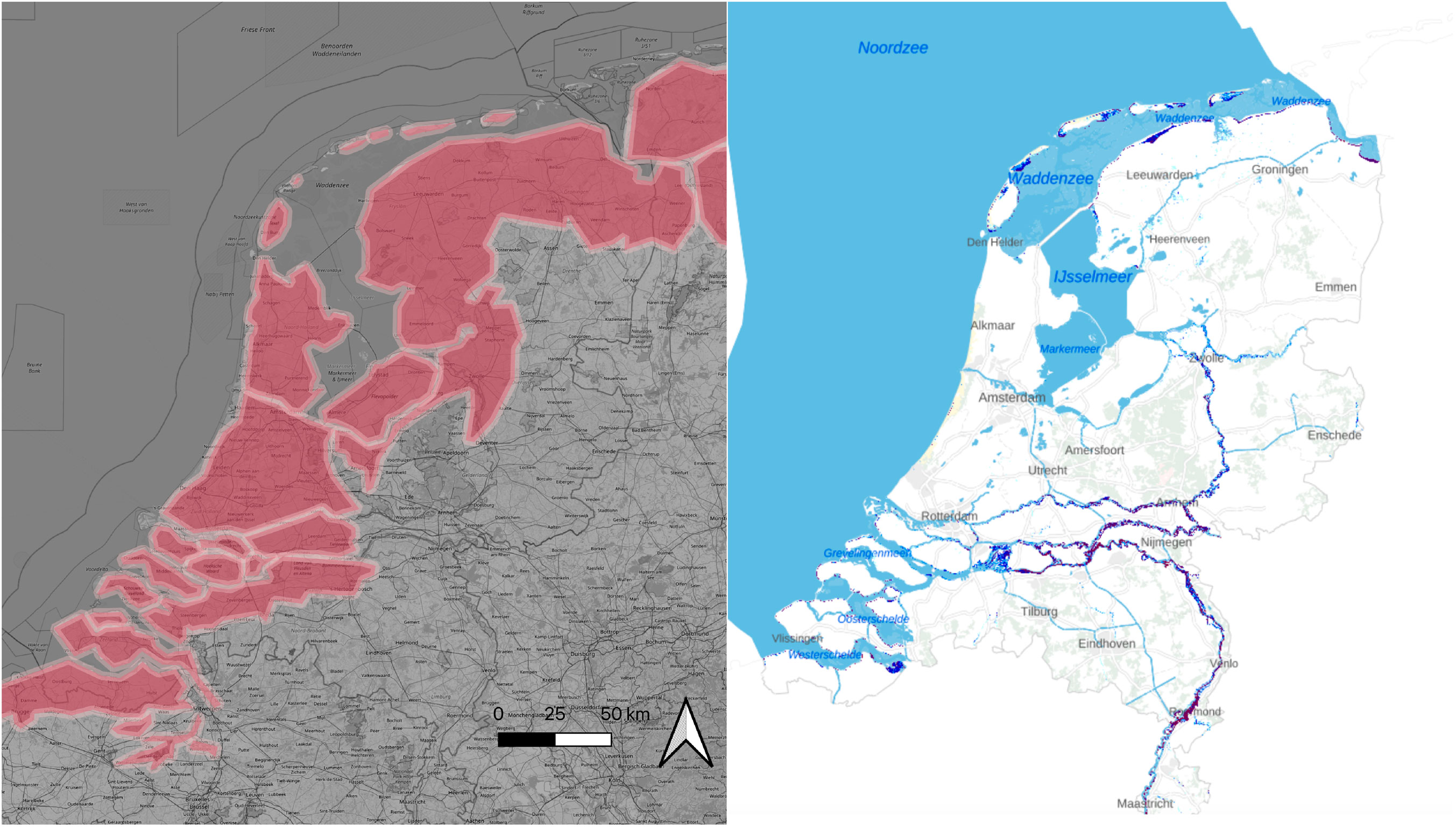
Figure 1. Two coastal flooding maps. Left: global scenario from CoastalDEM (Dataset (Kulp and Strauss, 2019), Map analogue to Climate Central (Central, 2024) (return period 10 years, sketched due to copyright restrictions, background map by OpenStreetMap), Right: local scenario from Landelijk Informatiesysteem Water en Overstromingen (LIWO), from the responsible government authority Rijkswaterstaat (mosaic of scenarios with return periods of 10 years).

In the global approach (Figure 1 - left panel), a large part of the country is flooded, while in the local approach (Figure 1 - right panel), only the river flood banks are affected. Interpreting these maps leads to vastly different conclusions, which can cause concerns as they are not only used in scientific and media contexts but also in political discussions (e.g., House Committee on Natural Resources Committee, 2020).

This raises the question of which map is “true.” How can these two maps, based on the same return period flood, vary so much? What explains the differences, and how can we quickly understand them?

Many fields have struggled with models that need an accessible and brief annotation. A common solution is to find a short, understandable notation that defines which methodology was applied. Often a simple linguistic or semiotic notation is used to provide a convention about the technical details. Table 1 provides a few examples.

Table 1

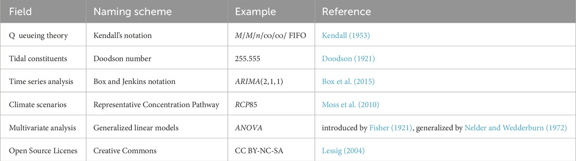
Table 1. Examples of notation conventions for various fields.

This study provides an overview of the current methodological choices for assessing susceptibility to flooding and introduces a summarizing notation that reflects these choices. To describe the current methods for assessing flood susceptibility, this study first shows the general workflow. The available methods, approaches, and corresponding datasets offer considerations for methodological choices in each component. These choices affect the resulting flood map, and thus its suitability for certain uses. The case study shows this sensitivity for an example region. The discussion section reflects on the suitability of different choices for a set of applications.

2 Methods

To define a workflow and corresponding annotation for creating coastal flood susceptibility maps, global coastal flooding studies such as (Gutenson et al., 2017; Jongman et al., 2012; Kulp and Strauss, 2019; Neumann et al., 2015) were reviewed.

The common steps in these studies provide the basis for the proposed workflow and corresponding annotation. It is important to note that not all steps are present in all studies. In some studies, the coastal defence step is absent, whereas other studies focus only on present or future scenarios, et cetera. These steps also form the name of the proposed annotation: Waterlevel, Elevation, Protection, Flood, Impact, Future (WEPFIF).

Waterlevel

A first decision is the water level to use. Coastal flooding can only occur if the water level of the sea exceeds the local land level.

Elevation

The second decision concerns which land elevation to use. Elevation determines the area susceptible to flooding and the path that the water will take.

Protection

Flooding can only occur when there are no barriers that prevent the water from overflowing the land: natural and man-made flood defences.

Flood

If the water indeed managed to pass by natural or man-made flood defences, a fourth decision concerns the way in which the water is assumed to reach the lower regions.

Impact

The societal impact step translates the hazard to risk using flood exposure and vulnerability (following Aitsi-Selmi et al., 2015).

Future

These maps are often made for the current situation but also for a potential future. This future can affect any of the steps. Section 3.6 discusses the choices for a future for all steps in the workflow. The combination of these choices for “the future” are often implemented as a scenario or storyline.

Figure 2 presents a visual format of the workflow. The directed connectivity shows that some elements are required for other elements. Water levels, bathymetry and coastal defence, are used as input to the flooding model. The flood extent generated by the flooding model is input to the societal impact assessment. As we will discuss both hard and soft protection we have used visualization of a coast with dunes, similar to the coast used in Section 4.

Figure 2

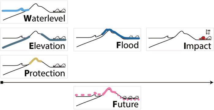
Figure 2. General workflow to generate a coastal flood map consisting of choosing how to represent Waterlevel (cyan blue), Elevation (metallic blue), Protection (tan) Flood model (denim), Impact (red) and possible Future (rose pink).

Section 3 expands the proposed WEPFIF workflow by providing notation for each of the steps using example studies, available datasets, and available models. Section 4 applies the proposed notation to a coastal town (Katwijk aan Zee, NL) and a low lying country (Netherlands).

3 The WEPFIF approach

3.1 W: Water level

The first choice in Figure 2 is which water/sea surface level to use. There are several relevant indicators for the height of the sea.

A systematic analysis by Hauer et al. (2020) shows that common sea-level indicators include (from low to high): Mean Sea Level (MSL), Mean High High Water (MHHW), or more general High Sea Level (HSL), a water level with a specific annual return period (e.g., 100 years, see Section 3.1.3 for a detailed discussion), and a fixed level of 10 m referred to as LECZ (originating from McGranahan et al., 2007).

In meso- and macro-tidal areas, tidal high water is an important precondition for flooding. That is why taking into account tide is important to evaluate the flood proneness. We refer to the sea-level including tides as HSL. There are different HSL’s. Common in the context of coastal flooding are Mean High High Water (MHHW) and Highest Astronomical Tide (HAT).

MHHW is the average height of the highest tide recorded each day over a certain observed period. The Highest Astronomical Tide (HAT) is the highest predicted astronomical tide expected to occur (in a 18.6 years cycle), which can be significantly higher than MHHW due to the amplitude magnification of the nodal tide (Baart et al., 2012).

In areas with a non-reflective gentle sloped coast the combination of storm surge and wave run-up is also an important factor for flooding. Including storm surge levels (without waves) can be referred to as Storm Surge Level (SSL). This typically includes both the inverse barometer effect (low pressure at the coast and high pressure offshore pushing the water towards the coast) and storm surges due to the wind forcing water towards the coast. Since 2020s studies (Vousdoukas et al., 2020b; Kirezci et al., 2020) have opted also to include waves. This can include wave set-up and wave run-up (see discussion Melet et al., 2018; Aucan et al., 2019). The sum of tides, storm surge and wave setup is commonly referred to as the eXtreme Sea Level (XSL). Both for surge and wave height one needs to define which surge/wave height to take into account. This is addressed in Section 3.1.3.

The motivations for selecting between different water levels can vary. Kulp and Strauss (2019) use MHHW and add a water height of 2 m as a representative water level corresponding to a “bad flood in the nearer term or an extreme sea-level scenario for 2,100”. Kirezci et al. (2020) aim to quantify the relative importance of tidal variations to potential episodic coastal flooding by 2,100. To do that they sum up surge, wave setup, and sea-level rise with event probabilities of $\frac{1}{100}$ per year.

3.1.1 Datasets

Relevant data sources for Absolute Mean Sea Level (AMSL) include the MSL product from the NASAs MEaSUREs program (Zlotnicki et al., 2019) or the similar product from Copernicus (Taburet and Pujol, 2021).

Relevant data sources for tide include the constituents datasets by the global tidal models TPXO (Egbert and Erofeeva, 2002) (available as open source/data up to version 7) and FES 2014 Carrère et al. (2016). These datasets are derived from satellite observations. Satellite observations only allow to resolve a limited number of tidal constituents due to their low revisit frequency ($O$(1 day⁻¹)), only allowing to estimate MHHW globally and not HAT. The alternative is to do tidal analysis on the water levels from coastal stations and interpolate and extrapolate these to a global dataset. For this purpose SOEST HAWAII archives high frequency tide ($<=\frac{1}{10}$min⁻¹) gauge measurements (see Piccioni et al., 2019, for an analysis of 1,145 records).

On top of the tidal water level a storm surge level can be included, and also wave setup. These are commonly denoted with their return period. A storm surge with a probability of occurring each year $\frac{1}{100}$yr⁻¹ is noted as a 100years storm surge. A global reanalysis dataset that includes coastal storm surges and also solves tidal constituents based on tidal forcings is provided by the GTSM reanalysis product (Muis et al., 2016; Dullaart et al., 2020). These, however, do not include density-driven circulations, which are important in the deeper, less mixed regions. There one would prefer ocean models. However, these models do not include tide or at least not on the same temporal scale as coastal models do. There are efforts ongoing to go towards a hybrid approach (Wang et al., 2022).

The combined effect of storm surge, wind and waves with an accurate free surface is implemented in local coastal models. In global applications waves, surge, and tides are often treated separately. Arns et al. (2020) showed that it is important not to just add the different components. Storm surge can be lower during high tide due to non-lineair interaction effects. Datasets for XSL include coastal global wave reanalysis datasets, such as Wave Watch III (Tolman, 2009). Excluding waves is sometimes referred to as the StillWater Level (SWL) (see FEMA, 2015).

A final aspect, which links this section with Section 3.2 is the choice of local reference level. There is a distinction between AMSL, the absolute sea-level relative to a geoid and Relative Mean Sea Level (RMSL), relative to a local benchmark connected to the solid earth. For coastal flooding the RMSL is important. To translate absolute sea-level to a local reference level one has to match datums. This is not always trivial. Global covering mean sea-level based on satellite measurements is referenced as an anomaly and local relative sea-level based on tide gauges is centrally collected as a revised local reference level. Although matching horizontal geospatial reference systems is well addressed by the central collection of the different projections in the European Petroleum Survey Group (EPSG) registry, connecting vertical reference levels can be quite challenging (Muis et al., 2017). One way to consistently connect global absolute sea level to local measured relative sea level is using Lowest Astronomical Tide (LAT) maps (Slobbe et al., 2013).

3.1.2 Codes

Based on the analysis of the inclusion of sea-surface height in coastal flooding models we come to the following coding for the methodological sections (see Figure 3). The wave and storm surge codes can make use of the extra subscript code discussed in Section 3.1.3.

Mean

Mean Sea Level (MSL)

Tide

MSL + Tide, High Sea Level (HSL), including high tidal level MHHW, MHHW, HAT

Surge

MSL + Ttide + Surge, Storm Surge Level (SSL) HSL including a return periods of storm surge

eXtreme

MSL + Ttide + Surge + Waves, eXtreme Sea Level (XSL), SSL including wave setup and or swash.

Fixed

Fixed heights, such as Lower Elevation Coastal Zone (LECZ), 10 m above MSL or geoid.

Figure 3

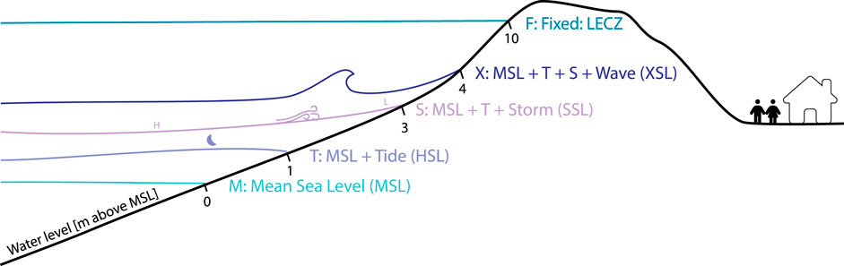
Figure 3. Waterlevel: different vertical sea surface levels used in the assessment of coastal flooding.

3.1.3 Subscript codes for probabilities of surge and waves

To estimate a representative surge or wave height, one of the challenges for a coastal flooding approach is how to deal with extreme weather events. One of the challenges with extreme events is that they are, per definition, rarely observed which makes it necessary to infer the probability of an event. There are different approaches to infer the probability:

For regions with tropical storms it is common to use a probability model based on observed or generated storm tracks (Knapp et al., 2010; Nederhoff et al., 2021). However, cyclones can miss a single location for several decades. Therefore local measurements of storm surge are not representative of the expected storm surge (see O’Grady et al., 2022, for a discussion and suggested approach). Resampling and generative techniques (e.g., Emanuel et al., 2006; Lin et al., 2012) can be employed to estimate storm surges for these specific types of storms. The extensive set of synthetic simulations generated in this process enables the utilization of both empirical and fitted extreme value distributions (Bloemendaal et al., 2020; Dullaart et al., 2021). For extra-tropical storms, it is common to use a parametric approach based on extreme value theory (de Haan, 1990), often based on local tide gauge measurements. Satellite measurements have a lower frequency (they might miss the highest storm surge) and are less accurate near the shore, where the highest storm surges occur.

There are two methods within the parametric approach. One uses a Generalized Extreme Value (GEV) distribution, with an annual maximum series (see Jenkinson (1955) for an early application; Lin et al. (2019) for a recent example). The other uses the Generalized Pareto Distribution (GPD) with a Peak Over Threshold (POT) approach (see Pickands (1975) for an early example; Vousdoukas et al. (2016a) for a recent example). Both methods can be used to infer the probability distribution of unseen extreme events. The annual maxima approach works better with historic data (Baart et al., 2011), because only the maximum of a year is needed. This makes it better suitable for using historical records. The POT method requires more measurements, hourly or higher frequency. See Caires (2016) for a recent comparison. See also Wahl et al. (2017) for an overview of the sources of variations in XSL.

Extensions can include conditional probabilities using a Bayesian approach (Calafat and Marcos, 2020), spatial dependence (the probability of an extreme event to occur in nearby locations) and temporal dependence (the probability of an event to occur twice) (Caires et al., 2011).

This overview gives us the following coding style for the choices of a probability model.

Synthetic

Generated data. For example, generated weather generator.

Annual Maximum

Fitted GEV distribution using the Annual Maxima (AM) method on observed data.

Peak Over Threshold

Fitted GPD distribution using a Peak Over Threshold (POT) method on observed data.

Similar to the fixed height we suggest to use the return period in years as a postfix to this notation. For example, $S10$ refers to a 10 years return period based on synthetic records.

3.2 E: Elevation

Topography selection is crucial for coastal flooding studies. A topographic dataset is referred to as a Digital Elevation Model (DEM). Two relevant subtypes are Digital Surface Model (DSM), which includes objects such as trees, buildings, and cars, and Digital Terrain Model (DTM), where these objects are filtered out (Hirt, 2014; Guth et al., 2021). Estimating bathymetry, sometimes called Digital Bathymetric Model (DBM), is also important for calculating how much energy reaches the coast. The intertidal bathymetry often combines topographic and bathymetric information. Many bathymetric survey efforts are part of the General Bathymetric Chart of the Oceans (GEBCO) initiative (Hall, 2006). This section focuses on the terrain aspect of elevation modelling, where there is less convergence.

3.2.1 Datasets

The first globally measured DEM at 1 arc minute resolution ($O$(30 m) at the equator) became available through the Shuttle Radar Topography Mission (SRTM) (Rabus et al., 2003) dataset. This dataset was measured in February 2000 using synthetic aperture radars aboard the NASA Space Shuttle Endeavour. It allowed to create more detailed hypsometric curves (as defined by Harrison et al., 1981), which confirmed that the lower elevated coastal areas, between (between −6 and 6 m), are less steep and therefore extra sensitive to sea-level rise. The SRTM (a DSM) served as the base for many later generations of DEMs, using ever better filtering techniques and using more ancillary datasets, moving slowly towards a global high resolution DTM. The latest reprocessing by NASA is the NASADEM, which is enhanced using ICESAT and other global DEMs (Crippen et al., 2016). Table 2 presents commonly used DEMs with their type.

Table 2

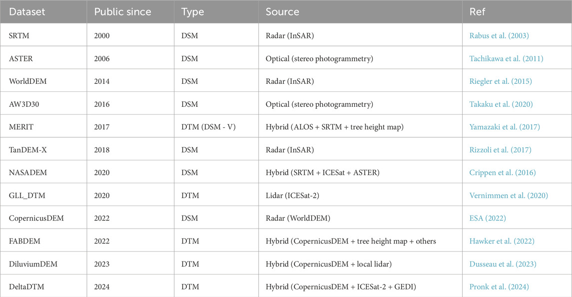
Table 2. Overview of DEM datasets (closed datasets in gray), commonly used in overland flooding computations.

There are three measurement sources for global height estimates (optical, radar and laser). A recent development is hybrid DEMs, where multiple sensors are combined. The first global covering DTMs based on ICESAT-2 appear, but the derived grids still have a coarse resolution, due to the wide interswath distance of the profile-based LIDAR measurements. For coastal flooding, it is important to take into account buildings, vegetation and trees. The Multi-Error-Removed Improved-Terrain (MERIT) dataset (Yamazaki et al., 2017) was the first to incorporate global tree height estimates.

An evaluation of datasets for coastal flooding applications (Gesch, 2018) concluded that none of these global DEMs are sufficiently accurate for modelling fine increments of Sea-Level Rise (SLR) ($<1$m) over short planning horizons ($<100$yr). The new hybrid DEMs try to evolve from a DSM to a DTM by removing vegetation, trees, and buildings. These improvements in the workflow improve the accuracy for coastal flooding to the order of 3 m (Gesch, 2018) (see also Uuemaa et al. (2020) for a detailed analysis of the accuracy), which is still a multiple of common sea-level rise scenarios (e.g., Hawker et al., 2018; Winsemius et al., 2019). The latest DEMs try to incorporate the latest global covering high resolution spaceborne lidar (Ice, Cloud, and land Elevation Satellite (ICESat)-2) to enhance the accuracy (Dusseau et al., 2023; Pronk et al., 2024).

3.2.2 Codes

For the elevation part of the workflow, the codes are defined based on which elements are included and excluded in the DEM. A coastal flooding map user should quickly discern whether a DSM or DTM is used, and in intermediate cases, what has been filtered out. This leads to the following notation for this component (see also Figure 4).

Surface

Digital Surface Model (DSM)

Surface - Vegetation

Digital Surface Model (DSM) minus canopy (tree tops) and (optional) other vegetation, also referred to as Non Vegetated Surface (NVS) (Guth et al., 2021).

Surface - Buildings

Surface minus buildings

Terrain

Digital Terrain Model (DTM), Digital Surface Model (DSM) minus vegetation and buildings and objects (e.g., infrastructure).

Figure 4

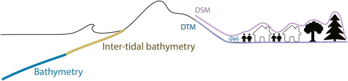
Figure 4. Elevation choice, schematic representation of the Digital Terrain Model (DTM) (green) versus Digital Surface Model (DSM) (rose) and the possible options (vegetation, objects, buildings, canopy) that can be optionally subtracted.

3.3 P: Protection

The comparison of two cases with similar water levels but different flooding levels, shown in Figure 1, illustrates that next to sea surface height and topography, ignoring features that impede the influx of water can have a significant impact on the end result. The scenario based on CoastalDEM (Kulp and Strauss, 2019; Central, 2024) did not include coastal protection measures. In countries with robust coastal protection policies (clear policy targets, strong accompanying funding arrangements, effective maintenance organisation and emergency response), low-lying areas can still have very high levels of protection. These protection levels may be the result of hard infrastructural measures, like dikes, dams, storm surge barriers, etc., or well-maintained natural protective features, such as dune areas, tidal flats, salt marshes, mangroves, reefs, etc.

Natural dunes defend a large part of the Dutch coast. Dunes are “soft” coastal protections. Den Heijer et al. (2012) showed that the Dutch dune coast mostly offers very high levels of protection. The weak sections of the coast have since been upgraded. An intricate system of dike rings provides further protection and compartmentalisation of the low-lying areas, reducing the risk even further (see for example, Eijgenraam, 2007). The peaks of coastal dunes do not show up in digital terrain models, because of the limited resolution.

The Dutch coast is also protected by “hard” coastal protection. Examples include the new hard-fixed sea wall on the Afsluitdijk and the parking garage in a dune near Katwijk that provides extra coastal protection (Al, 2022). Breakwaters near Rotterdam and IJmuiden shield the inlets from the waves. Some of these coastal protections can be seen in the topography or bathymetry, but only with sufficient resolution. Some hard protections are movable. A very visible, but only during extreme water levels, example is the Maeslantkering (Mooyaart and Jonkman, 2017). Other countries have also used movable coastal defense structures, the MOSE barriers at Venice Italy (delle Acque, 1997), the Thames barrier (Kendrick, 1988), and the concept of the Ike Dike (Torres et al., 2017) are examples. These storm surge barriers provide temporary protection during high water, but this function is not directly discernible from a DTM. Smaller scale, movable protection measures include coupures in levees and openings that can be closed by a gate or by placing segments when high water is imminent.

These two types of protection measures (soft, hard) in combination with dynamic flooding routines make all the difference in the area considered actually prone to flooding a country like the Netherlands. When you do include these it also makes sense to include the potential failure of these defense systems. Hurricane Katrina showed that dike systems are only as strong as their weakest link (Jonkman et al., 2009). Despite the presence of dyke systems in the US, and the availability of a highly skilled organisation like the United States Army Corps of Engineers, an extreme event like a hurricane still caused a large part of the region to be flooded. In the aftermath, coastal protection policies were reviewed and strengthened. There are many studies that focus on the potential of protection using structures, such as sea walls and dikes (Hinkel et al., 2014; Tiggeloven et al., 2020) and on using nature-based solutions (Beck et al., 2018; Menéndez et al., 2020; Van Coppenolle and Temmerman, 2020; de Vries et al., 2021; van Zelst et al., 2021).

Some coastal flood risk models are specifically designed to support climate adaptation decisions. These studies often compute the needed disaster risk reduction as an economic decision problem [as proposed by van Dantzig (1956)]. Due to the limited empirical data on actual implemented defence and adaptation (Hinkel et al., 2014), assuming a ‘protection level’ is a common approach. Lincke and Hinkel (2018) give an overview of where coastal adaption is a robust investment. Using a similar approach Vousdoukas et al. (2020a) show that economically efficient adaptation can reduce 83% of the coastal flooding.

3.3.1 Datasets

Depending on the type of coastal protection, different datasets are needed to take it into account. Which dataset is relevant depends on the size of the features and with which sensor they can be recognized. Submerged coastal protection (submerged breakwaters, shoreface nourishments) is only visible with detailed underwater surveys and is missing from many global covering bathymetries due to the lack of resolution. The same is true for features in the topography. Large dune areas may be detected, but more minor features such as levees or sea walls may not show up in global covering DTMs. Even more difficult are the movable protective measures, which can only be seen during the extreme high water levels that they were designed for. It is possible to accurately map intertidal vegetation and inland marshes using Sentinel 1 images (de Vries et al., 2018). Land cover maps intended for inland purposes, such as the Corine Land Cover map EEA (2018) are not always accurate enough in the nearshore. For both hard and soft coastal protection a promising approach is to use the information collected by the OpenStreetMap community. They have started to register coastal structures such as breakwaters. This type of information can be used directly or as a source of training and validation data for object detection (see e.g., Wing et al., 2019).

When detailed maps of coastal protection are not available one can assume that some coastal protection is in place. For this purpose, one can use the FLOod PROtection Standards (FLOPROS) (Scussolini et al., 2016), which builds on the earlier work of Hallegatte et al. (2013). To give a rough estimate of flood return periods Hinkel et al. (2014) provide estimates. This approach assumes that coastal defences will not fail below their design return period.

3.3.2 Codes

The codes for this section, as visualized in Figure 5, assume that you can include information on the Soft and Hard protection level directly into your flood model. The alternative is to assume that a whole region can only be flooded based on a certain Protection Level.

Soft

Soft coastal protection. This can include surface roughness that mitigates the extent of a flood or wave propagation.

Hard

Hard coastal protection. This can include flood mitigating constructions such as flood barriers.

Protection Level

Floods are assumed to not occur below a certain protection level.

Figure 5

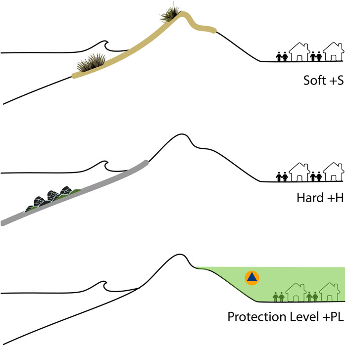
Figure 5. Protection method choices. Soft protection (e.g., surface roughness, in light brown) and hard protection (e.g., flood barriers, in grey) versus a general assumed protection level (in light green).

3.4 F: Flood

For flooding assessment a range of methods is available, ranging from pure Geographic Information System (GIS) operations to highly detailed numerical flood modelling. The earliest global analysis of flood risk (Nicholls et al., 1999) used a simple approach in 192 coastal zones globally. They assumed a coastal plane with a constant slope per assessment zone, and used that to calculate inundation. The development of global covering high-resolution topography and bathymetry (as discussed in Section 3.2) allows for a wider repertoire of flooding methods (Vousdoukas et al., 2016b).

The simplest approach to flood models are the so-called bathtub models (Williams and Lück-Vogel, 2020). They are also known as static, equilibrium or planar surface projection models and are sometimes referred to as “GIS-based”. In this context, GIS based refers to that the maps can be made using standard GIS software (for example, using GDAL, SAGA in QGIS, Google Earth Engine, or ArcGIS). These methods are based on spatial operations on vector or raster maps. The term static refers to that the flooding occurs instantaneously, and the duration is not taken into account. The advantage of these models is that they do not take dependencies between neighbouring areas into account and scale up very well, as they are suitable for map-reduce operations commonly used in the cloud. They can be considered worst-case scenarios.

The bathtub approach can also include more information on the local roughness. An example of including roughness to limit flooding is given by Vafeidis et al. (2019); Ward et al. (2020). They artificially steepened the DEM land slopes to mimic roughness that limits water fluxes. The land use determined by satellite data is used to make a spatially varying change to the local slope. The Euclidean distance of each DEM point to the sea is shortened with this factor. After this mapping, calculating the flood exposure is in the GIS domain again. They report 44% less inundation exposure, using the method sometimes referred to as the “sloped coast” method.

Because the pure “bathtub” approach does not consider connectivity between adjacent cells, a cell can flood even if not connected to the flood source. In this approach, polders and other low-lying areas near the coast get flooded. Some studies correct this by removing unconnected flood cells in a post-processing step (Muis et al., 2016), which brings us to the following approach.

To overcome the issue that water floods the area behind coastal protection (as seen in the two lower left figures in Figure 6) methods that we refer to as “connectivity” methods can be used, sometimes referred to as semi-dynamic. An example application was presented by Poulter and Halpin (2008). They compared three flooding methods, all based on geometric operations on a raster. The static bathtub method, in the connectivity world referred to as the zero-side rule, was compared to two methods that can take into account obstacles. Poulter and Halpin (2008) considered the 4-sided and 8-sided rule. In these connectivity methods, a cell can only flood if the extreme water level can reach the cell via the 4 lateral sides or also via its diagonal connections. The latter methods are said to take care of hydrological connectivity. This calculation is harder to split up as subdomains need to communicate to their neighbour if their boundary is flooded (see Breilh et al., 2013; Williams and Lück-Vogel, 2020, for discussion).

Figure 6

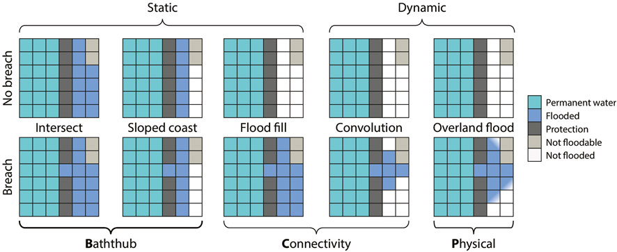
Figure 6. Five different flood methods under two conditions (closed coastal defence and open coastal defence). The sea is located on the left of the map. Blue areas are flooded. The dark grey area is coastal protection, higher than any water level. The light grey area is an inland area higher than the current water level. White areas are not flooded.

A downside of both these static methods is that they can lead to an overestimation of the flooded area of up to 200% (Vousdoukas et al., 2016b), see also Ramirez et al. (2016) for a broader discussion. Figure 6 also makes this clear. Water reaches areas that are not flood-prone (top left two). The connectivity (middle bottom) result can be reached. Here, the problem is that this ‘flood fill’ method does not take into account the limited duration of a storm and high tide. If it finds a ‘hole’ in the coastal defence, it will instantly fill the entire flood-prone area, while in reality, the peak of the event under which flooding occurs might be over in 6 hours, and to be able to reach far inland, water needs to overcome roughness (vegetation, buildings).

An example of a simple approach to including the concept of time is given by Dottori et al. (2018). They apply the assumption that the discharge of water over a dyke/weir is limited by laws of physics, described by the excess water level compared to the dyke height in an empirical formula. Using the storm duration and its water level variations therein - the design hydrograph - this leads to a cap on the volume that can flood the area. The hydrograph limits flood duration, and so the total flood water volume is limited. The second factor leading to attenuation of the flooding is resistance experienced by the flood wave, via bed roughness or obstructions of the flow path. We refer to methods that assume connectivity and limit the flood extent as “convolution” methods, as they tend to require an iteration of a convolution step.

The most realistic approach, but also the most computationally intensive and requiring the most input data, is to use a reduced complexity “physical” models based on hydrodynamics, such as LISFLOOD-FP (Bates et al., 2010). Also promising for global flooding applications is the SFINCS model Leijnse et al. (2021), which is fast, can deal with compound flooding (river + coastal) and also includes wave run-up over dunes or dykes. One can also use traditional 2D overland flooding models, such as Mike 2D overland flooding, 3Di or Delft3D Flexible Mesh. Still, these are harder to set up and require more computation hours because they also contain physics, such as advection, that are less relevant during a flood. New approaches promise to speed up computation time (van den Bout et al., 2023).

More advanced models do exist that also take into account erosion, the possibility of dune and dike failure, and flooding due to groundwater (sunny day flooding). These have been applied on a national scale but not yet on a global scale. There have been recent developments towards machine learning-based methods to compute flood extends (see Jones et al., 2023, for an overview). The creation of flood-specific datasets can help to estimate flood extents without physics-based models and without the need for oversimplification (e.g., Bonafilia et al., 2020).

Despite efforts to establish benchmarks for coastal flooding (Nederhoff et al., 2024; Néelz and Pender, 2013) and pluvial flooding (Aerts et al., 2020), a need remains for a structured, community-driven intercomparison benchmark specifically for coastal flooding. Jafarzadegan et al. (2023) also highlighted the weak and selective validation of flood inundation models and the lack of sufficient validation data. They also discuss the balance between accuracy, reliability versus computationally efficiency.

Finding the balance between applicability, scalability, explainability, computation time, and model setup is a reason why there is not one dominant method. The baththub based approach is also still evolving, Kasmalkar et al. (2024) try to address the overestimation of flooding by baththub models by including hydraulic connectivity and path-based attenuation. In Artificial intelligence (AI) based approaches the connectivity models are also used as one of the input features or as a reference (e.g., Jones et al., 2023).

3.4.1 Models

Depending on the flood model used one needs different data sources. For the bathtub model, one only needs an integrated DBM, DSM (as discussed in Section 3.2). For models that also include connectivity, it becomes more relevant to include coastal protection (as discussed in Section 3.3). The dynamic models also require roughness maps. For the nearshore and intertidal zones, these maps were discussed under the soft protection section in Section 3.3. That section also gives an overview of inland land use maps (which can be converted to roughness using model-specific tables). Here we provide an overview of hydrodynamic models suitable for global applications, using raster input, with short runtimes (in the order of minutes for a year simulation time, for a $1x1$km² area).

Examples of models that are commonly used in physics-based coastal flooding include Lisflood-FP (Bates et al., 2010), Mike21 (Warren and Bach, 1992), D-Hydro (Delft3D, SOBEK) (Kernkamp et al., 2011), SFINCS (Leijnse et al., 2021), and XBeach (Roelvink et al., 2009). Software commonly used for connectivity and bathtub simulations is GRASS (Neteler et al., 2012), QGIS (Samela et al., 2018), ArcGIS or Google Earth Engine (Gorelick et al., 2017).

3.4.2 Codes

Based on the description above we come to the following code notation for flood models.

Bathtub

Bathtub methods, also referred to as static methods.

Connectivity

Connectivity based methods that take into account coastal protection.

Phyiscal

Physics-based flooding models that limit the flood by taking into account roughness and or time resulting in a reduction of the mass and momentum of the flood.

3.5 I: Impact

Flood risk is defined as the product of hazard, exposure, and vulnerability (e.g., Aitsi-Selmi et al., 2015). Following the definitions of United Nations Office for Disaster Risk Reduction (UNDRR) hazard is “A process, phenomenon or human activity that may cause loss of life, injury or other health impacts, property damage, social and economic disruption or environmental degradation.” (Author, 2016). Exposure is “The situation of people, infrastructure, housing, production capacities and other tangible human assets located in hazard-prone areas.”. Vulnerability is “The conditions determined by physical, social, economic and environmental factors or processes which increase the susceptibility of an individual, a community, assets or systems to the impacts of hazards.”.

The hazard in coastal flooding entails the seawater over-flooding the shore, typically quantified with a probability of a certain flood extent. Exposure entails the economic assets and people in that in the flood-prone area. Vulnerability refers to the predisposition of a community to suffer harm when exposed to a hazard, based on aspects like social, economic, and environmental factors that influence the ability to cope with and recover from a flood. The hazard component is a result of the flood computations described in the previous sections. This section focuses on the societal impact of a flood and the result: exposure times vulnerability. De Moel et al. (2015) and Botzen et al. (2019) provide an extended overview of aspects to take into account while assessing exposure and vulnerability. Staupe-Delgado (2019) gives an overview on how the terminology has evolved over time and the challenges around ambiguity.

Flood exposure is typically quantified with metrics of the population, the urban area, or economic assets that are exposed (see Figure 7) to a flood with a certain probability (e.g. Muis et al., 2017). The area at risk is the easiest to determine. It is determined by the results of the flooding model defined in Section 3.4. Areas already underwater (rivers, streams, lakes, reservoirs) should be excluded from the potentially flooded area. Population maps are needed to estimate the population living in flood-prone areas (see for example, Edmonds et al., 2020). Estimating the value that is flood prone is the most laborious. This requires the express cost of the property. Some use a more simple approach by assuming that Gross Domestic Product (GDP) is uniformly distributed over the population. The population maps can then be used as a measure of asset value (e.g., Kirezci et al., 2020). One can also refine the distribution of house prices. For example, properties close to the coast tend to be more valuable, referred to as the “coastal premium” (see e.g., Conroy and Milosch, 2011; Ling, 2021).

Figure 7

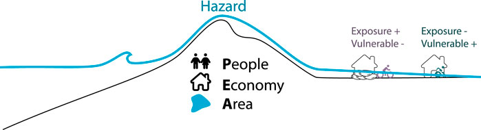
Figure 7. Impact of coastal flooding: indicators in common use (People affected, Economic damages, Area affected). Presented in the context of the hazard of a storm on the left and exposure and vulnerability of the population depicted on the right.

Flood vulnerability is a step further. Here one should consider how the flooded areas are affected by a flood. Coastal regions may become saltier after coastal flooding. That “loss of function” type of evaluation is mainly applied on a local scale (e.g., Storlazzi et al., 2015), rarely in global studies. Not all regions that get flooded are vulnerable. Many people choose to live in flood-prone areas because the land is more fertile, it is closer to economic activity (e.g., near ports), et cetera. People tend to be aware of a potential flood and are prepared, thus their vulnerability is low.

A flood can also have indirect consequences. The consequences of the consequences, such as the Fukushima disaster (Hollnagel and Fujita, 2013) show us that the indirect effects of a flood can sometimes be more severe than the direct effects. To do this on a global covering scale is not realistic at the moment, because it requires integrated information on complex systems. Rising sea levels and flooding can lead to increased groundwater levels and salinity. This rise in salinity can significantly reduce the suitability of water for agriculture and drinking purposes (as discussed by e.g., Youssef et al., 2021).

3.5.1 Datasets

Table 3 gives an overview of relevant datasets to assess impact and vulnerability.

Table 3

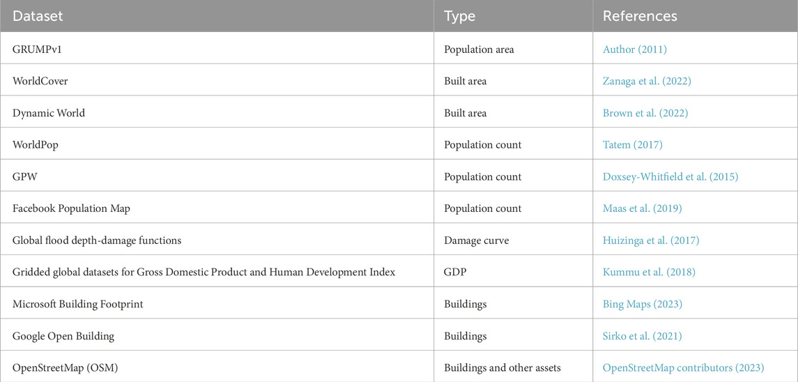
Table 3. Overview of datasets for global covering vulnerability and exposure assessment.

3.5.2 Codes

The codes for the societal impact of floods are the following:

People

People at risk. Loss of life. Number of evacuees.

Economy

Damages to assets, value. Loss of culture. Criticality effects.

Area

Area susceptible to flooding.

3.6 F: Future

The “future” label in the WEPFIF notation outlines the incorporation of future changes into the coastal flooding workflow. Typically, this process involves duplicating a workflow and adjusting the input parameters to account for various scenarios. The section comprehensively breaks down how to include future scenarios in each component.

3.6.1 Water level

Future sea surface height is typically taken into account using one of the IPCC scenarios (Pörtner et al., 2022) or their regional equivalents (e.g., Wuebbles et al., 2017). For the notation it is important to denote which scenario is used and which quantities from these scenarios are used, for example, one could use ${MSL}_{\mathit{SSP5-8.5}}$ for a scenario where future mean sea-level from the Shared Socioeconomic Pathways (SSP) with radiative forcing of 8.5 W m² is used. Or one could have ${MSL}_{\mathit{SSP5-8.5}}+W_{\mathit{SSP5-8.5}}$ if both mean sea level and wave setup are derived from SSP5-8.5 scenarios. The AR6 IPCC report (IPCC, 2022) uses the Scenario Matrix Architecture, which combines the SSPs and the Representative Concentration Pathway (RCP)s (Riahi et al., 2017). Future sea-surface height can also change due to changes in storm surge climate or tidal amplitude.

3.6.2 Elevation

Vertical land motion, driven by various factors such as groundwater or gas extraction, can also be included. Some sources have localized effects lasting years to decades (Gerardo et al., 2021). provides an overview map of these sources. An important source of subsidence is the Glacio Isostatic Adjustment (GIA), a global effect. Peltier (2004) provides the basis for commonly used maps that correct for this. There is an ongoing effort to link tide gauge records to Global Navigation Satellite System (GNSS) based estimates of vertical land motion (Woodworth et al., 2017), which allows estimates in coastal regions using methods based on broken regression models (e.g., Oelsmann et al., 2022).

3.6.3 Protection

For future sea level, it is important to also take into account that many coasts around the world are gaining land due to coastal maintenance and gaining or losing land due to sediment flows (Luijendijk et al., 2018). Sea-level rise can also lead to erosion in deltas, based on (Bruun, 1962) and follow-up studies.

Next to the current levels of protection, the projection of future policies is relevant to creating future flood maps. One can not be certain which countries will improve their coastal defence in the future, but for 90% of the people, it will be the most effective strategy (Lincke and Hinkel, 2018), even under the highest sea-level scenarios. Hinkel et al. (2014) showed how important it is to include future coastal protection. Flood damages by the end of this century are most sensitive to the applied protection strategy. Lomborg (2020) concluded that because not all coastal flood maps take protection into account, coastal impacts are often “vastly exaggerated”. Aspects to take into account for future protection are:

Future protection level

Will all parts of the coast have the same protection level, or will spatial planning result in increased or reduced protection levels? This allows for more optimized resource allocation.

Future Impact

This can change due to population and land development changes caused by migration and population increase or decrease.

Expected lifetime

Protection measures have an expected lifetime and can degrade over time.

Investment strategy

Governments can vary in how much they invest in coastal protection infrastructure. How can these strategies evolve over time?

Technological innovation

One can expect future innovations. The efficiency with which one can do coastal protection measures and the availability of solutions can increase.

McEvoy et al. (2021) found that in 75% of the European countries future sea-level rise is already taken into account in coastal maintenance and spatial planning strategies. Most of the countries use IPCC scenarios as a basis for their estimate of sea-level rise in 2,100. There is a skewness towards the use of high-end scenarios: RCP2.6 is used by 13 countries, 18 countries use RCP4.5, and 22 countries use RCP8.5.

The protection levels within a country (defined as the return period of the representative design event) tend to be consistent over time. They are often chosen based on the economic value behind the coastal protection. If the economic value changes faster or slower than the cost of improving coastal protection one could opt to reconsider the protection level. What can change is the lifetime of coastal protection if sea-level rise is higher or lower than when estimated during construction. When the sea-level rise is higher than expected, the end-of-life of coastal protection will be reached faster than anticipated.

A challenge for taking into account future scenarios is also to know the local long term protection policy. In the Netherlands, as part of the 2^nd Deltaprogramme (Kabat et al., 2009), the current levels of safety and protection are foreseen to be maintained for many years to come using a “hold the line” strategy, where coastal erosion is to be countered with sand nourishment. In the UK, with its much larger area and longer coastline, it is not feasible to apply the same level of protection everywhere. In less densely populated areas a managed retreat strategy, or managed realignment strategy, is actively considered and implemented. This also implies that in such cases, the realigned areas become more prone to flooding, in line with the local long-term protection policy. Some areas in the world are left partially open to flooding to increase the ecological function of a region (Cox et al., 2006).

3.6.4 Impact

Coastal flood risk assessments are typically forward-looking and focus on how risk may change in the future. In addition to the use of climate change scenarios to estimate future flood hazards, the use of future socio-economic scenarios is widespread. In general, the socio-economic changes have been driving increases in coastal flood risk over the last decades (Jongman et al., 2012), while for future projection the extra concern of increased hazard due to increase in extreme water levels is important (Vousdoukas et al., 2018b). Some have started towards local projections of future vulnerabilities (Hardy and Hauer, 2018). Vulnerabilities can reduce over time due to measures such as innovations in building design, evacuation plans, early warning systems or decrease if a more vulnerable part of the population moves toward the coast (see Tanoue et al., 2016, for an example in river flooding).

4 Case study

This section applies the workflow on country and town level to the Netherlands, shown in Figure 8. The town of Katwijk aan Zee is vulnerable to sea-level rise (Al, 2022), has a combination of different topographic elements (dunes, town) and a drainage lock structure which also serves as coastal defense. Netherlands is a flat polder Delta, which is sensitive to accuracy of DEM and was presented in Figure 1.

Figure 8

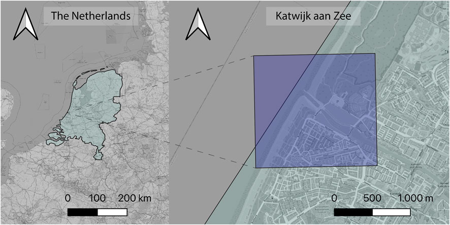
Figure 8. Regions (left: the Netherlands $O(100km)$, right: Katwijk aan Zee $O(1000m)$) that are used as a case study to show the WEPFIF approach.

The goal of zooming into the coastal town of Katwijk is to show the detailed effect of including protection in global flood studies. Zooming out to the Netherlands shows the effect of a DEM sensitive region (low lying polder) on countrywide indicators, by varying water level, elevation, and flood method.

To show the sensitivity of the WEPFIF choices Figure 9 presents three common flooding method (baththub, connected 4 sided, connected 8 sided), combined with a subset of six global DEM datasets compared with the local lidar measurements of Actueel Hoogtebestand Nederland (AHN)2 as reference, to the country of the Netherlands. The top left figure is equivalent to a hypsometric curve (area on the x-axis as a function of water level on the y-axis). The bold codes in ${\mathit{W}}_{\mathit{y}}{\mathit{E}}_{\mathit{lines}}P{\mathit{F}}_{\mathit{row}}{\mathit{I}}_{\mathit{column}}F$ varied. The variation in flooded area and population as a function of water level shows how sensitive these results are to the chosen DEM. The DEM are less reliable for lower water levels, especially below 4 m.

Figure 9

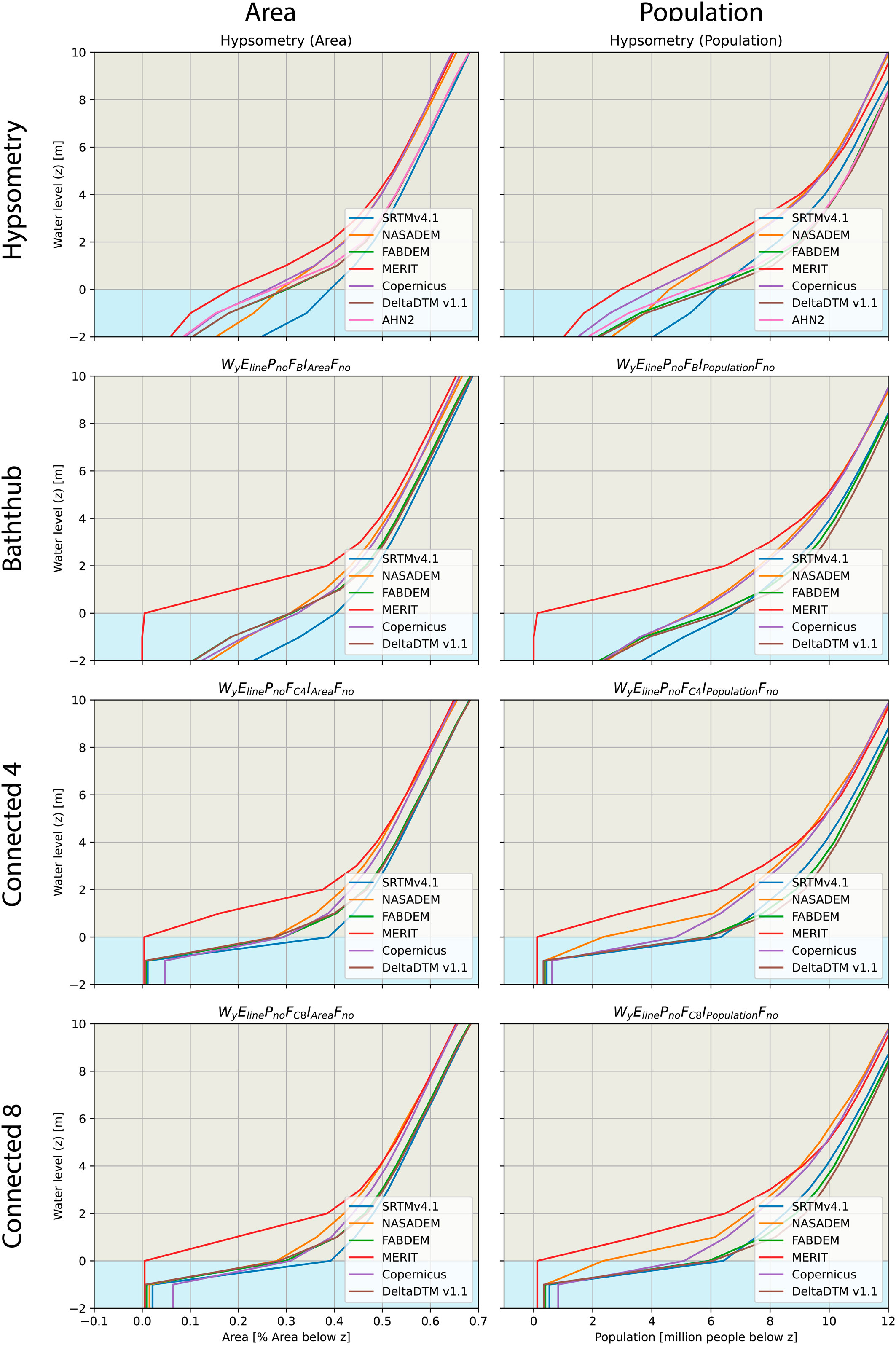
Figure 9. Variation in flooded area (left column) and flooded population (right column) as a function of water level (y-axis) and flooding method (rows).

Figure 10 shows the zoomed in perspective on the town of Katwijk aan Zee. In this analysis we compare different flood scenarios based on (Riahi et al., 2017; van Dorland et al., 2024) (SSP5-8.5 based scenario with Marine Ice Cliff Instability (MICI) (note Morlighem et al., 2024) included, here referred to as SSP5-8.5+) with the same set of DEMs as in Figure 9. The figure shows the large variation in flooded area under the parameters (design storm surge with extreme scenario). If the recently upgraded coastal defense structure (which is not detected by most of the global DEMs) is included and combined with a scenario in line with current emissions (Hausfather and Peters, 2020). The flooded areas are more moderate, more consistent between DEMs and more in line with the high resolution reference DEM of AHN2. The bold codes varied in this example: ${\mathit{W}}_{\mathit{row3vs4}}{\mathit{E}}_{\mathit{column}}{\mathit{P}}_{\mathit{row4vs5}}{\mathit{F}}_{\mathit{row3vs4}}I{\mathit{F}}_{\mathit{row3vs4vs5}}$.

Figure 10

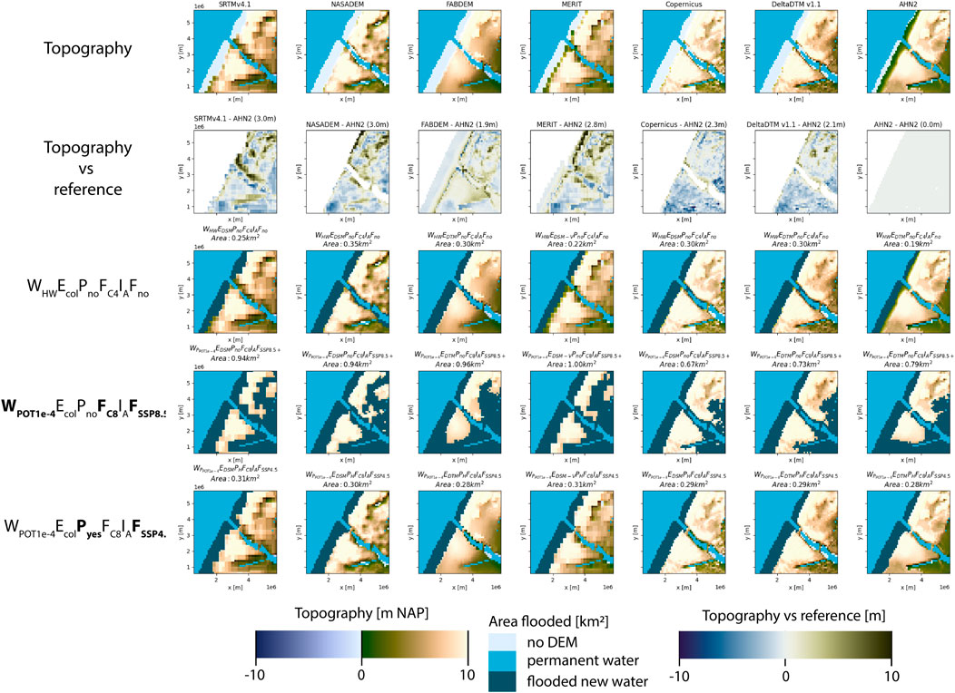
Figure 10. First row shows the topography of selected DEM’s. The second row shows the difference and RMSE compared to the reference topography (AHN2) in the last column. The third rows shows a reference scenario representing the current state $W_{HW}{E}_{\mathit{columns}}{P}_{no}{F}_{C4}{I}_{A}Fno$. The fourth row shows a $\frac{1}{10000}$ per year storm surge combined with the fossil fueled plus Antarctic collapse scenario $W_{\mathit{POT1e-4}}{E}_{\mathit{columns}}{P}_{no}{F}_{C8}{I}_A{F}_{\mathit{SSP8.5+}}$. The fifth row shows the effect of the same extreme storm surge, with hard protection included, with the road divided scenario $(W_{\mathit{POT1e-4}}{E}_{\mathit{columns}}{P}_H{F}_{C8}{I}_A{F}_{\mathit{SSP4.5}})$.

5 Discussion and conclusion

5.1 Coastal flooding method notation: a step to help compare local and global flooding models

Most of the technical challenges to generate global hyper-resolution coastal-flooding impact studies have been addressed over the last decade. It is now possible to generate maps with resolutions of 30 m or higher by combining several publicly available datasets. Thus, the new challenge is not only achieving global coverage and high resolution but also ensuring local relevance (see e.g. Gianinazzi, 2018). To be locally actionable, one needs to be able to compare results with local studies. For this, it is important to know which methodological choices have been made.

To facilitate the task of defining and determining the details of these methodological choices, this study presents a workflow with an accompanying semantic coding scheme for coastal flooding applications. This coding scheme can help to do a comparison between global and local studies or between different studies of the same spatial extent. The notation assigns codes to each of the six steps in the workflow of a coastal flood risk calculation: the land elevation (Section 3.2) that will flood (Section 3.4) from the sea (Section 3.1) if not properly protected (Section 3.3), resulting in societal impact (Section 3.5), now or in the future (Section 3.6).

For each of the steps in the workflow methodological choices can be noted using the coding scheme.

Waterlevel

$M\to$ Mean Sea Level (MSL), $T\to M+$ Tide, $S\to T+$ Storm surge, $X\to S+$ Waves, $F\to$ Fixed level.

Elevation

$S\to$ Digital Surface Model (DSM), $S-C\to$ canopy filtered out, $S-V\to$ vegetation (other than trees) filtered out, $S-B\to$ Buildings filtered out, $T\to$ Digital Terrain Model (DTM)

Protection

$S\to$ Soft, $H\to$ Hard, $PL\to$ Protection level.

Flood

$B\to$ Baththub, $C\to$ Connectivity, $P\to$ Physical.

Impact

$P\to$ People, $E\to$ Economic, $A\to$ Area.

Future

Depending on applications, for example, $SSP5-8.5_{2100}$

5.2 Method meets objective

The application of this coding scheme to a collection of coastal studies illustrates how it can be used. Table 4 shows the wide variation of choices that studies make in their methods.

Table 4

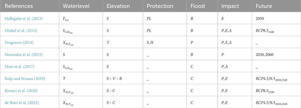
Table 4. Overview of coastal flooding studies annotated using the Waterlevel, Elevation, Protection, Flood, Impact, Future (WEPFIF) notation.

The research objective of each study in Table 4, particularly in relation to quantifying current and future impacts, elucidates the contextual differences in the applied methodologies. Hallegatte et al. (2013) quantify potential future economic loss due to climate change to provide advice on adaption policy. Hinkel et al. (2014) estimate future damages and adaptation costs to support efforts to reduce emissions. Vergouwe (2014) estimates current flood risk in the Netherlands. Muis et al. (2017) estimate the current risk of coastal flooding to assess how much risk could be avoided if flood protection standards were increased. Kulp and Strauss (2019) improve exposure estimates to inform coastal communities that the future is more difficult than previously thought. Kirezci et al. (2020) estimate future episodic floods to show the massive environmental and socio-economic impacts.

The goals of these studies and their typical methodological considerations can be summarized in a general recommendation. In all cases, employing a DTM appears more advantageous than a DSM, as reflected in the preference for a $E=T$ choice.

The state of the world

The reflective, summarizing approach to the current and future state of the world with respect to coastal flooding benefits most from a variation of methodological choices. Here, one typically looks at water levels with locally relevant (corresponding to policy) return periods to show the likelihood of certain events. The future is less relevant: one can focus on the current state of the system. To show a realistic image, one wants to include flood protection, but given the limited availability of coastal protection datasets, a protection level approach could suffice for now. One could use a dynamic flood method that considers whether water can retreat back to the coast after a flood. Impact indicators for area and people are most relevant. In summary a $S_{\mathit{AM100}}:T:S,H:P:P,A$: model ($W=S_{\mathit{AM100}}$, $E=T$, $P=P{L}_{100}$, $F=P$, $I=P,A$, $F=none$) would be an applicable example.

Optimizing investment

When choosing to replace coastal protection one often looks at a water level with a return period corresponding to a local criteria. This rarely includes waves, but often includes tidal amplitude, which can also vary over time. The main challenge is to determine which regions will not be floodable. A connectivity-based method can suffice for global studies. It is important to know the current state of coastal protection and potential future investment. Both protection and future protection should be estimated. The impact on economic value (also incorporating ecological and cultural value) is relevant. For the future, one can assume that the sea level will rise. Therefore, at least future mean sea-level changes should be estimated. One could consider leaving out scenarios deemed less plausible (Pielke Jr et al., 2022). To summarize a $T_{\mathit{AM100}}:T:S,H:C:P,E:SSP2-45$ model ($W=X_{\mathit{AM100}}$, $E=T$, $P=S,H$, $F=P$, $I=P,E$, $F=SSP2-45$) would be an applicable example.

Raising concern

Raising awareness is not enough, so more dramatic flood images should be created, some argue (e.g., Luccioni et al., 2021). Here one can also use an XSL, with waves including. One can further dramatize the flood images by presenting the future state under the assumption of “inactivity”, with or without the current flood protection. Combining these assumptions with a bathtub-based flooding model gives the greatest potential flooded maps. The population affected is then the most common output indicator. For this purpose, the SSP5-8.5 future scenario is most often used. There are ethical dilemmas to consider: Will people have a realistic level of concern when presented with a selective subset of information? Is it the scientists’ role to influence people’s level of concern? In summary a $X_{\mathit{AM100}}:T::B:P:SSP5-85$ model ($W=X_{\mathit{AM100}}$, $E=T$, $P=none$, $F=B$, $I=P$, $F=SSP5-85$) would fit this purpose.

This overview shows different considerations for the choices based on the different objectives of the global coastal flooding studies. This large variation corresponds to the large variation in methods, which points out how important it is to elaborate and notate these choices but also the corresponding goal clearly.

5.3 Data, models and tools

Not only does the research goal determine the choices made, but also the availability of open and Findable Accessible Interoperable Reusable (FAIR) datasets and computing resources influences which choices can be made within the time available for a study. Unfortunately, many of the tools, models, and model schematizations are still not available under an open-source license. This makes it difficult to build upon the work of others. Examples from the studies above include the CoastalDEM dataset, the tidal model TPXO, the model schematization of the GTSM, and the Dynamic Interactive Vulnerability Assessment (DIVA) impact model; none of these are available under an open-source license. When data is open, it is not always easy to use. For example. For example, the GTSM reanalysis data is available through the Copernicus portal, but it can not be downloaded as a whole. One has to make several small requests to access the data, which violates the FAIR principles.

Physics-based flooding models that can be used for global applications are available, but there is a lack of a public global schematization that can be used. This is why most studies fall back to the bathtub or connectivity methods; they need large amounts of data to set up an alternative approach. Some of the data just has not been collected on a global scale. There is no high resolution ($O(30)$m) global covering reproducible DTM available. There have been some efforts to make a dataset of protection levels, but no dataset that covers hard and soft coastal defence is available. There is no dataset available on current and future protection investment strategies. This makes it impossible to create future scenarios based on the realistic assumption that people will defend their coasts as the sea level rises.

5.4 Concluding remarks

This paper provides an overview of methodological approaches in recent global coastal flooding impact studies. To enhance comparability, it introduces the WEPFIF coding scheme. Applying this scheme, the study demonstrates the reasons for inconsistencies between results. Achieving consistent and explainable results is crucial as we stand on the brink of shifting from theoretical global evaluations to actionable local-level information.

This is the first approach to a coding scheme for coastal flooding studies. It encourages others to improve upon it, create variations, or extend it based on studies not included in this analysis or when new methodological choices are introduced. Like other coding schemes, it will need to adapt as methodology progresses. Scientists are encouraged to extend or simplifythe suggested approach.

Data availability statement

Publicly available datasets were analyzed in this study. The datasets were used from the copies at the following locations. AHN: https://developers.google.com/earth-engine/datasets/catalog/AHN_AHN2_05M_INT; MERIT: https://developers.google.com/earth-engine/datasets/catalog/MERIT_DEM_v1_0_3; Copernicus DEM: https://developers.google.com/earth-engine/datasets/catalog/COPERNICUS_DEM_GLO30; NASA SRTM: https://developers.google.com/earth-engine/datasets/catalog/USGS_SRTMGL1_003; DeltaDTM: https://data.4tu.nl/datasets/1da2e70f-6c4d-4b03-86bd-b53e789cc629; FABDEM GEE: https://gee-community-catalog.org/projects/fabdem/; GDEM GEE project: https://gee-community-catalog.org/projects/aster/.

Author contributions

FB: Investigation, Data curation, Software, Validation, Visualization, Writing–original draft, Writing–review and editing. GB: Investigation, Data curation, Software, Validation, Visualization, Writing–original draft, Writing–review and editing. MP: Investigation, Data curation, Software, Validation, Writing–review and editing. MK: Investigation, Writing–review and editing. SM: Investigation, Writing–review and editing.

Funding

The author(s) declare that financial support was received for the research, authorship, and/or publication of this article. This research was partially funded by the subsidy for Institutes for Applied Research (BWBR0040605).

Conflict of interest

Authors GB and MK were employed by Van Oord.

The remaining authors declare that the research was conducted in the absence of any commercial or financial relationships that could be construed as a potential conflict of interest.

Publisher’s note

All claims expressed in this article are solely those of the authors and do not necessarily represent those of their affiliated organizations, or those of the publisher, the editors and the reviewers. Any product that may be evaluated in this article, or claim that may be made by its manufacturer, is not guaranteed or endorsed by the publisher.

References

Aerts, J. P. M., Uhlemann-Elmer, S., Eilander, D., and Ward, P. J. (2020). Comparison of estimates of global flood models for flood hazard and exposed gross domestic product: a China case study. Nat. Hazards Earth Syst. Sci. 20, 3245–3260. doi:10.5194/nhess-20-3245-2020

CrossRef Full Text | Google Scholar

Aitsi-Selmi, A., Egawa, S., Sasaki, H., Wannous, C., and Murray, V. (2015). The sendai framework for disaster risk reduction: renewing the global commitment to people’s resilience, health, and well-being. Int. J. Disaster Risk Sci. 6, 164–176. doi:10.1007/s13753-015-0050-9

CrossRef Full Text | Google Scholar

Al, S. (2022). Multi-functional urban design approaches to manage floods: examples from Dutch cities. J. Urban Des. 27, 270–278. doi:10.1080/13574809.2021.1977112

CrossRef Full Text | Google Scholar

Almar, R., Ranasinghe, R., Bergsma, E. W. J., Diaz, H., Melet, A., Papa, F., et al. (2021). A global analysis of extreme coastal water levels with implications for potential coastal overtopping. Nat. Commun. 12, 3775. doi:10.1038/s41467-021-24008-9

PubMed Abstract | CrossRef Full Text | Google Scholar

Arns, A., Wahl, T., Wolff, C., Vafeidis, A. T., Haigh, I. D., Woodworth, P., et al. (2020). Non-linear interaction modulates global extreme sea levels, coastal flood exposure, and impacts. Nat. Commun. 11, 1918. doi:10.1038/s41467-020-15752-5

PubMed Abstract | CrossRef Full Text | Google Scholar

Aucan, J., Hoeke, R. K., Storlazzi, C. D., Stopa, J., Wandres, M., and Lowe, R. (2019). Waves do not contribute to global sea-level rise. Nat. Clim. Change 9, 2. doi:10.1038/s41558-018-0377-5

CrossRef Full Text | Google Scholar

Author, U. (2011). Global rural-urban mapping project, version 1 (grumpv1): Population count grid

Google Scholar

Author, U. (2016). Report of the open-ended intergovernmental expert working group on indicators and terminology relating to disaster risk reduction. report

Google Scholar

Baart, F., Bakker, M. A. J., van Dongeren, A., den Heijer, C., van Heteren, S., Smit, M. W. J., et al. (2011). Using 18th century storm-surge data from the Dutch coast to improve the confidence in flood-risk estimates. Nat. Hazards Earth Syst. Sci. 11, 2791–2801. doi:10.5194/nhess-11-2791-2011

CrossRef Full Text | Google Scholar

Baart, F., van Gelder, P. H. A. J. M., de Ronde, J., van Koningsveld, M., and Wouters, B. (2012). The effect of the 18.6-year lunar nodal cycle on regional sea-level rise estimates. J. Coast. Res. 28, 511–516. doi:10.2112/JCOASTRES-D-11-00169.1

CrossRef Full Text | Google Scholar

Bates, P. D., Horritt, M. S., and Fewtrell, T. J. (2010). A simple inertial formulation of the shallow water equations for efficient two-dimensional flood inundation modelling. J. Hydrology 387, 33–45. doi:10.1016/j.jhydrol.2010.03.027

CrossRef Full Text | Google Scholar

Beck, M. W., Losada, I. J., Menéndez, P., Reguero, B. G., Díaz-Simal, P., and Fernández, F. (2018). The global flood protection savings provided by coral reefs. Nat. Commun. 9, 2186. doi:10.1038/s41467-018-04568-z

PubMed Abstract | CrossRef Full Text | Google Scholar

Bloemendaal, N., de Moel, H., Muis, S., Haigh, I. D., and Aerts, J. C. J. H. (2020). Estimation of global tropical cyclone wind speed probabilities using the storm dataset. Sci. Data 7, 377. doi:10.1038/s41597-020-00720-x

PubMed Abstract | CrossRef Full Text | Google Scholar

Bonafilia, D., Tellman, B., Anderson, T., and Issenberg, E. (2020). “Sen1floods11: a georeferenced dataset to train and test deep learning flood algorithms for sentinel-1,” in 2020 IEEE/CVF conference on computer vision and pattern recognition workshops (CVPRW), 835–845. doi:10.1109/CVPRW50498.2020.00113

CrossRef Full Text | Google Scholar

Borrego, C. (1990). Integrated coastal zone strategy: need for a more quantitative approach, 15. WIT Transactions on Ecology and the Environment.

Google Scholar

Botzen, W. J. W., Deschenes, O., and Sanders, M. (2019). The economic impacts of natural disasters: a review of models and empirical studies. Rev. Environ. Econ. Policy 13, 167–188. doi:10.1093/reep/rez004

CrossRef Full Text | Google Scholar

Box, G. E., Jenkins, G. M., Reinsel, G. C., and Ljung, G. M. (2015). Time series analysis: forecasting and control. John Wiley and Sons.

Google Scholar

Breilh, J. F., Chaumillon, E., Bertin, X., and Gravelle, M. (2013). Assessment of static flood modeling techniques: application to contrasting marshes flooded during xynthia (western France). Nat. Hazards Earth Syst. Sci. 13, 1595–1612. doi:10.5194/nhess-13-1595-2013

CrossRef Full Text | Google Scholar

Brown, C. F., Brumby, S. P., Guzder-Williams, B., Birch, T., Hyde, S. B., Mazzariello, J., et al. (2022). Dynamic world, near real-time global 10 m land use land cover mapping. Sci. Data 9, 251. doi:10.1038/s41597-022-01307-4

CrossRef Full Text | Google Scholar

Bruun, P. (1962). Sea-level rise as a cause of shore erosion. J. Waterw. Harb. Div. 88, 117–130. doi:10.1061/jwheau.0000252

CrossRef Full Text | Google Scholar

Caires, S. (2016). A comparative simulation study of the annual maxima and the peaks-over-threshold methods. J. Offshore Mech. Arct. Eng. 138. doi:10.1115/1.4033563

CrossRef Full Text | Google Scholar

Caires, S., De Haan, L., and Smith, R. (2011). On the determination of the temporal and spatial evolution of extreme events. Deltares Rep. 1202120-001-HYE-0004 Rijkswaterstaat, Waterdienst

Google Scholar

Calafat, F. M., and Marcos, M. (2020). Probabilistic reanalysis of storm surge extremes in europe. Proc. Natl. Acad. Sci. 117, 1877–1883. doi:10.1073/pnas.1913049117

PubMed Abstract | CrossRef Full Text | Google Scholar

Carrère, L., Lyard, F., Cancet, M., and Guillot, A. (2016). “Fes 2014, a new tidal model—validation results and perspectives for improvements,” in Proceedings of the ESA living planet symposium, 9–13.

Google Scholar

Central, C. (2024). Interactive global map showing areas threatened by sea level rise and coastal flooding. Map.

Google Scholar

Conroy, S. J., and Milosch, J. L. (2011). An estimation of the coastal premium for residential housing prices in san diego county. J. Real Estate Finance Econ. 42, 211–228. doi:10.1007/s11146-009-9195-x

CrossRef Full Text | Google Scholar

Cox, T., Maris, T., De Vleeschauwer, P., De Mulder, T., Soetaert, K., and Meire, P. (2006). Flood control areas as an opportunity to restore estuarine habitat. Ecol. Eng. 28, 55–63. doi:10.1016/j.ecoleng.2006.04.001

CrossRef Full Text | Google Scholar

Crippen, R., Buckley, S., Agram, P., Belz, E., Gurrola, E., Hensley, S., et al. (2016). Nasadem global elevation model: methods and progress. Int. Archives Photogrammetry, Remote Sens. Spatial Inf. Sci. XLI-B4, 125–128. doi:10.5194/isprs-archives-XLI-B4-125-2016

CrossRef Full Text | Google Scholar

van Dorland, R., Beersma, J., Bessembinder, J., Bloemendaal, N., van Den Brink, H., Brotons Blanes, H., et al. (2024). KNMI national climate scenarios 2023 for The Netherlands. report [dataset]

Google Scholar

de Boer, G., Oudman, E., Danebjer, L., Jawaid, Z., Tosun, G., Terry, R., et al. (2022). Climate risk overview. Rapid Glob. Sel. Clim. Adapt. Oppor.

Google Scholar

de Haan, L. (1990). Fighting the arch–enemy with mathematics. Stat. Neerl. 44, 45–68. doi:10.1111/j.1467-9574.1990.tb01526.x

CrossRef Full Text | Google Scholar

delle, A. (1997). Interventi alle bocche lagunari per la regolazione dei flussi di marea# studio di impatto ambientale del progetto di massima

Google Scholar

de Moel, H., Jongman, B., Kreibich, H., Merz, B., Penning-Rowsell, E., and Ward, P. J. (2015). Flood risk assessments at different spatial scales. Mitig. Adapt. Strategies Glob. Change 20, 865–890. doi:10.1007/s11027-015-9654-z

PubMed Abstract | CrossRef Full Text | Google Scholar

den Heijer, C., Baart, F., and van Koningsveld, M. (2012). Assessment of dune failure along the Dutch coast using a fully probabilistic approach. Geomorphology 143-144, 95–103. doi:10.1016/j.geomorph.2011.09.010

CrossRef Full Text | Google Scholar

de Vries, M., van der Wal, D., Möller, I., van Wesenbeeck, B., Peralta, G., and Stanica, A. (2018). Earth Observation Coast. Zone Glob. images local Inf. FP7 FAST Proj. syntesis Rep. (Zenodo). doi:10.5281/zenodo.1158437

CrossRef Full Text | Google Scholar

de Vries, M., van Koningsveld, M., Aarninkhof, S., and de Vriend, H. (2021). Objectifying building with nature strategies: towards scale-resolving policies. Res. Urbanism Ser. 7, 51–72. doi:10.47982/rius.7.128

CrossRef Full Text | Google Scholar

Doodson, A. T. (1921). The harmonic development of the tide-generating potential. Proc. R. Soc. Lond. Ser. A-Containing Pap. a Math. Phys. Character 100, 305–329.

Google Scholar

Dottori, F., Martina, M. L. V., and Figueiredo, R. (2018). A methodology for flood susceptibility and vulnerability analysis in complex flood scenarios. J. Flood Risk Manag. 11, S632–S645. doi:10.1111/jfr3.12234

CrossRef Full Text | Google Scholar

Doxsey-Whitfield, E., MacManus, K., Adamo, S. B., Pistolesi, L., Squires, J., Borkovska, O., et al. (2015). Taking advantage of the improved availability of census data: a first look at the gridded population of the world, version 4. Pap. Appl. Geogr. 1, 226–234. doi:10.1080/23754931.2015.1014272

CrossRef Full Text | Google Scholar

Dullaart, J. C. M., Muis, S., Bloemendaal, N., and Aerts, J. C. J. H. (2020). Advancing global storm surge modelling using the new era5 climate reanalysis. Clim. Dyn. 54, 1007–1021. doi:10.1007/s00382-019-05044-0

CrossRef Full Text | Google Scholar

Dullaart, J. C. M., Muis, S., Bloemendaal, N., Chertova, M. V., Couasnon, A., and Aerts, J. C. J. H. (2021). Accounting for tropical cyclones more than doubles the global population exposed to low-probability coastal flooding. Commun. Earth and Environ. 2, 135. doi:10.1038/s43247-021-00204-9

CrossRef Full Text | Google Scholar

Dusseau, D., Zobel, Z., and Schwalm, C. R. (2023). Diluviumdem: enhanced accuracy in global coastal digital elevation models. Remote Sens. Environ. 298, 113812. doi:10.1016/j.rse.2023.113812

CrossRef Full Text | Google Scholar

Edmonds, D. A., Caldwell, R. L., Brondizio, E. S., and Siani, S. M. O. (2020). Coastal flooding will disproportionately impact people on river deltas. Nat. Commun. 11, 4741. doi:10.1038/s41467-020-18531-4

PubMed Abstract | CrossRef Full Text | Google Scholar

EEA (2018). Corine land cover (clc) 2018, version 20b2. Release Date 21-12-2018. doi:10.2909/960998c1-1870-4e82-8051-6485205ebbac

CrossRef Full Text | Google Scholar

Egbert, G. D., and Erofeeva, S. Y. (2002). Efficient inverse modeling of barotropic ocean tides. J. Atmos. Ocean. Technol. 19, 183–204. doi:10.1175/1520-0426(2002)019<0183:eimobo>2.0.co;22.0

CrossRef Full Text | Google Scholar

Eijgenraam, C. J. J. (2007). From optimal to practical safety standards for dike-ring areas. Water Sci. Technol. 56, 113–124. doi:10.2166/wst.2007.543

PubMed Abstract | CrossRef Full Text | Google Scholar

Emanuel, K., Ravela, S., Vivant, E., and Risi, C. (2006). A statistical deterministic approach to hurricane risk assessment. Bull. Am. Meteorological Soc. 87, 299–314. doi:10.1175/BAMS-87-3-299

CrossRef Full Text | Google Scholar

ESA (2022). Copernicus dem - global and european digital elevation model (cop-dem). Dataset. doi:10.5270/ESA-c5d3d65

CrossRef Full Text | Google Scholar

FEMA (2015). Guidance for flood risk analysis and mapping. Tech. Rep. FEMA.

Google Scholar

Fisher, R. A. (1921). Studies in crop variation. i. an examination of the yield of dressed grain from broadbalk. J. Agric. Sci. 11, 107–135. doi:10.1017/S0021859600003750

CrossRef Full Text | Google Scholar

Gerardo, H.-G., Pablo, E., Roberto, T., Marta, B.-P., Juan, L.-V., Mauro, R., et al. (2021). Mapping the global threat of land subsidence. Science 371, 34–36. doi:10.1126/science.abb8549

CrossRef Full Text | Google Scholar

Gesch, D. B. (2018). Best practices for elevation-based assessments of sea-level rise and coastal flooding exposure. Front. Earth Sci. 6, 230. doi:10.3389/feart.018.00230

CrossRef Full Text | Google Scholar

Gianinazzi, W. (2018). Penser global, agir local. histoire d’une idée. EcoRev’ 46, 19–30. doi:10.3917/ecorev.046.0019

CrossRef Full Text | Google Scholar

Gorelick, N., Hancher, M., Dixon, M., Ilyushchenko, S., Thau, D., and Moore, R. (2017). Google earth engine: planetary-scale geospatial analysis for everyone. Remote Sens. Environ. 202, 18–27. doi:10.1016/j.rse.2017.06.031

CrossRef Full Text | Google Scholar

Gutenson, J. L., Follum, M. L., Snow, A. D., and Wahl, M. D. (2017). Large-scale flood inundation modeling in data sparse environments using tandem-x terrain data. Open Water J. 4 (4).

Google Scholar

Guth, P. L., Van Niekerk, A., Grohmann, C. H., Muller, J.-P., Hawker, L., Florinsky, I. V., et al. (2021). Digital elevation models: terminology and definitions. Remote Sens. 13, 3581. doi:10.3390/rs13183581

CrossRef Full Text | Google Scholar

Hall, J. K. (2006). Gebco centennial special issue –charting the secret world of the ocean floor: the gebco project 1903–2003. Mar. Geophys. Res. 27, 1–5. doi:10.1007/s11001-006-8181-4

CrossRef Full Text | Google Scholar

Hallegatte, S., Green, C., Nicholls, R. J., and Corfee-Morlot, J. (2013). Future flood losses in major coastal cities. Nat. Clim. Change 3, 802–806. doi:10.1038/climate1979

CrossRef Full Text | Google Scholar

Hardy, R. D., and Hauer, M. E. (2018). Social vulnerability projections improve sea-level rise risk assessments. Appl. Geogr. 91, 10–20. doi:10.1016/j.apgeog.2017.2.019

CrossRef Full Text | Google Scholar

Harrison, C., Brass, G., Saltzman, E., Sloan, J., Southam, J., and Whitman, J. (1981). Sea level variations, global sedimentation rates and the hypsographic curve. Earth Planet. Sci. Lett. 54, 1–16. doi:10.1016/0012-821x(81)90064-9

CrossRef Full Text | Google Scholar

Hauer, M., Hardy, D., Kulp, S., Mueller, V., Wrathall, D., Clark, P., et al. (2020). A framework for classifying and assessing sea level rise risk. SocArXiv Pap. doi:10.31235/osf.io/tf6rj

CrossRef Full Text | Google Scholar

Hauer, M. E., Hardy, D., Kulp, S. A., Mueller, V., Wrathall, D. J., and Clark, P. U. (2021). Assessing population exposure to coastal flooding due to sea level rise. Nat. Commun. 12, 6900. doi:10.1038/s41467-021-27260-1

PubMed Abstract | CrossRef Full Text | Google Scholar

Hausfather, Z., and Peters, G. P. (2020). Emissions – the ‘business as usual’ story is misleading. Nature 577, 618–620. doi:10.1038/d41586-020-00177-3

PubMed Abstract | CrossRef Full Text | Google Scholar

Hawker, L., Bates, P., Neal, J., and Rougier, J. (2018). Perspectives on digital elevation model (dem) simulation for flood modeling in the absence of a high-accuracy open access global dem. Front. Earth Sci. 6, 233. doi:10.3389/feart.2018.00233

CrossRef Full Text | Google Scholar

Hawker, L., Uhe, P., Paulo, L., Sosa, J., Savage, J., Sampson, C., et al. (2022). A 30 m global map of elevation with forests and buildings removed. Environ. Res. Lett. 17, 024016. doi:10.1088/1748-9326/ac4d4f

CrossRef Full Text | Google Scholar

Hersbach, H., Bell, B., Berrisford, P., Hirahara, S., Horányi, A., Muñoz-Sabater, J., et al. (2020). The era5 global reanalysis. Q. J. R. Meteorological Soc. 146, 1999–2049. doi:10.1002/qj.3803

CrossRef Full Text | Google Scholar

Hill, C., DeLuca, C., Suarez, M., and Da Silva, A. (2004). The architecture of the earth system modeling framework. Comput. Sci. Eng. 6, 18–28. doi:10.1109/MCISE.2004.1255817

CrossRef Full Text | Google Scholar

Hinkel, J., Lincke, D., Vafeidis, A. T., Perrette, M., Nicholls, R. J., Tol, R. S. J., et al. (2014). Coastal flood damage and adaptation costs under 21st century sea-level rise. Proc. Natl. Acad. Sci. 111, 3292–3297. doi:10.1073/pnas.1222469111

PubMed Abstract | CrossRef Full Text | Google Scholar

Hirt, C. (2014). “Digital terrain models,”. Cham: Springer International Publishing. chap. 11. 1–6. doi:10.1007/978-3-319-02370-0_31-1

CrossRef Full Text | Google Scholar

Hoch, J. M., Neal, J. C., Baart, F., van Beek, R., Winsemius, H. C., Bates, P. D., et al. (2017). Glofrim v1. 0–a globally applicable computational framework for integrated hydrological–hydrodynamic modelling. Geosci. Model Dev. 10, 3913–3929. doi:10.5194/gmd-10-3913-2017

CrossRef Full Text | Google Scholar

Hollnagel, E., and Fujita, Y. (2013). The fukushima disaster – systemic failures as the lack of resilience. Nucl. Eng. Technol. 45, 13–20. doi:10.5516/NET.03.2011.078

CrossRef Full Text | Google Scholar

Hoozemans, F., Marchand, M., and Pennekamp, H. (1993). A global vulnerability analysis: vulnerability assessment for population, coastal wetlands and rice production on a global scale. Tech. Rep. H1588, Waterloopkundig Lab.

Google Scholar

House Committee on Natural Resources Committee (2020). “Ocean climate action: solutions to the climate crisis,” in Tech. rep. Washington, D. C.: Congress: House Committee on Natural Resources Committee.

Google Scholar

Hoyer, S., and Hamman, J. (2017). xarray: Nd labeled arrays and datasets in python. J. Open Res. Softw. 5, 10. doi:10.5334/jors.148

CrossRef Full Text | Google Scholar

Huizinga, J., de Moel, H., and Szewczyk, W. (2017). “Global flood depth-damage functions: methodology and the database with guidelines,” in JRC working papers JRC105688. Brussels, Belgium: Joint Research Centre (Seville site).

Google Scholar

IPCC (2022). “Climate change 2022: impacts, adaptation and vulnerability,” in Summary for policymakers. Cambridge, UK and New York, USA: CambridgeUniversity Press.

Google Scholar

Jafarzadegan, K., Moradkhani, H., Pappenberger, F., Moftakhari, H., Bates, P., Abbaszadeh, P., et al. (2023). Recent advances and new frontiers in riverine and coastal flood modeling. Rev. Geophys. 61, e2022RG000788. doi:10.1029/2022RG000788

CrossRef Full Text | Google Scholar

Jenkinson, A. F. (1955). The frequency distribution of the annual maximum (or minimum) values of meteorological elements. Q. J. R. Meteorological Soc. 81, 158–171. doi:10.1002/qj.49708134804

CrossRef Full Text | Google Scholar

Jones, A., Kuehnert, J., Fraccaro, P., Meuriot, O., Ishikawa, T., Edwards, B., et al. (2023). Ai for climate impacts: applications in flood risk. npj Clim. Atmos. Sci. 6, 63. doi:10.1038/s41612-023-00388-1

CrossRef Full Text | Google Scholar

Jongman, B., Ward, P. J., and Aerts, J. C. J. H. (2012). Global exposure to river and coastal flooding: long term trends and changes. Glob. Environ. Change 22, 823–835. doi:10.1016/j.gloenvcha.2012.07.004

CrossRef Full Text | Google Scholar

Jonkman, S. N., Maaskant, B., Boyd, E., and Levitan, M. L. (2009). Loss of life caused by the flooding of new orleans after hurricane katrina: analysis of the relationship between flood characteristics and mortality. Risk Anal. 29, 676–698. doi:10.1111/j.1539-6924.2008.01190.x

PubMed Abstract | CrossRef Full Text | Google Scholar

Kabat, P., Fresco, L. O., Stive, M. J. F., Veerman, C. P., van Alphen, J. S. L. J., Parmet, B. W. A. H., et al. (2009). Dutch coasts in transition. Nat. Geosci. 2, 450–452. doi:10.1038/ngeo572

CrossRef Full Text | Google Scholar

Kasmalkar, I., Wagenaar, D., Bill-Weilandt, A., Choong, J., Manimaran, S., Lim, T. N., et al. (2024). Flow-tub model: a modified bathtub flood model with hydraulic connectivity and path-based attenuation. MethodsX 12, 102524. doi:10.1016/j.mex.2023.102524

PubMed Abstract | CrossRef Full Text | Google Scholar

Kendall, D. G. (1953). Stochastic processes occurring in the theory of queues and their analysis by the method of the imbedded Markov chain. Ann. Math. Statistics 24, 338–354. doi:10.1214/aoms/1177728975

CrossRef Full Text | Google Scholar

Kendrick, M. (1988). The thames barrier. Landsc. Urban Plan. 16, 57–68. doi:10.1016/0169-2046(88)90034-5

CrossRef Full Text | Google Scholar

Kernkamp, H., Van Dam, A., Stelling, G., and de Goede, E. (2011). Efficient scheme for the shallow water equations on unstructured grids with application to the continental shelf. Ocean. Dyn. 61, 1175–1188. 1007/s10236-011-0423-6. doi:10.1007/s10236-011-0423-6

CrossRef Full Text | Google Scholar

Kirezci, E., Young, I. R., Ranasinghe, R., Muis, S., Nicholls, R. J., Lincke, D., et al. (2020). Projections of global-scale extreme sea levels and resulting episodic coastal flooding over the 21st century. Sci. Rep. 10, 11629. doi:10.1038/s41598-020-67736-6

PubMed Abstract | CrossRef Full Text | Google Scholar

Knapp, K. R., Kruk, M. C., Levinson, D. H., Diamond, H. J., and Neumann, C. J. (2010). The international best track archive for climate stewardship (ibtracs): unifying tropical cyclone data. Bull. Am. Meteorological Soc. 91, 363–376. doi:10.1175/2009BAMS2755.1

CrossRef Full Text | Google Scholar

Kulp, S. A., and Strauss, B. H. (2019). New elevation data triple estimates of global vulnerability to sea-level rise and coastal flooding. Nat. Commun. 10, 4844. doi:10.1038/s41467-019-12808-z

PubMed Abstract | CrossRef Full Text | Google Scholar

Kummu, M., de Moel, H., Salvucci, G., Viviroli, D., Ward, P. J., and Varis, O. (2016). Over the hills and further away from coast: global geospatial patterns of human and environment over the 20th–21st centuries. Environ. Res. Lett. 11, 034010. doi:10.1088/1748-9326/11/3/034010

CrossRef Full Text | Google Scholar

Kummu, M., Taka, M., and Guillaume, J. H. (2018). Gridded global datasets for gross domestic product and human development index over 1990–2015. Sci. data 5, 180004–180015. doi:10.1038/sdata.2018.4

PubMed Abstract | CrossRef Full Text | Google Scholar

Leijnse, T., van Ormondt, M., Nederhoff, K., and van Dongeren, A. (2021). Modeling compound flooding in coastal systems using a computationally efficient reduced-physics solver: including fluvial, pluvial, tidal, wind- and wave-driven processes. Coast. Eng. 163, 103796. doi:10.1016/j.coastaleng.2020.103796

CrossRef Full Text | Google Scholar

Lessig, L. (2004). The creative commons. Mont. L. Rev. 65, 1.

Google Scholar

Lichter, M., Vafeidis, A. T., Nicholls, R. J., and Kaiser, G. (2011). Exploring data-related uncertainties in analyses of land area and population in the “low-elevation coastal zone” (LECZ). J. Coast. Res. 27, 757–768. doi:10.2112/JCOASTRES-D-10-00072.1

CrossRef Full Text | Google Scholar

Lin, N., Emanuel, K., Oppenheimer, M., and Vanmarcke, E. (2012). Physically based assessment of hurricane surge threat under climate change. Nat. Clim. Change 2, 462–467. doi:10.1038/nclimate1389

CrossRef Full Text | Google Scholar

Lin, N., Marsooli, R., and Colle, B. A. (2019). Storm surge return levels induced by mid-to-late-twenty-first-century extratropical cyclones in the northeastern United States. Clim. Change 154, 143–158. doi:10.1007/s10584-019-02431-8

CrossRef Full Text | Google Scholar

Lincke, D., and Hinkel, J. (2018). Economically robust protection against 21st century sea-level rise. Glob. Environ. Change 51, 67–73. doi:10.1016/j.gloenvcha.2018.05.003

CrossRef Full Text | Google Scholar

Ling, Y. (2021). Estimating coastal premiums for apartment prices: towards a new multilevel modelling approach. Environ. Plan. B Urban Anal. City Sci. 49, 188–205. doi:10.1177/23998083211000343

CrossRef Full Text | Google Scholar

Lomborg, B. (2020). Welfare in the 21st century: increasing development, reducing inequality, the impact of climate change, and the cost of climate policies. Technol. Forecast. Soc. Change 156, 119981. doi:10.1016/j.techfore.2020.119981

CrossRef Full Text | Google Scholar

Luccioni, A., Schmidt, V., Vardanyan, V., and Bengio, Y. (2021). Using artificial intelligence to visualize the impacts of climate change. IEEE Comput. Graph. Appl. 41, 8–14. doi:10.1109/MCG.2020.3025425

PubMed Abstract | CrossRef Full Text | Google Scholar

Luijendijk, A., Hagenaars, G., Ranasinghe, R., Baart, F., Donchyts, G., and Aarninkhof, S. (2018). The state of the world’s beaches. Sci. Rep. 8, 6641. doi:10.1038/s41598-018-24630-6

PubMed Abstract | CrossRef Full Text | Google Scholar

Maas, P. (2019). “Facebook disaster maps: aggregate insights for crisis response & recovery,” in Proceedings of the 25th ACM SIGKDD International Conference on Knowledge Discovery & Data Mining (New York, NY: Association for Computing Machinery), KDD, 19. 3173. doi:10.1145/3292500.3340412

CrossRef Full Text | Google Scholar

MacManus, K., Balk, D., Engin, H., McGranahan, G., and Inman, R. (2021). Estimating population and urban areas at risk of coastal hazards, 1990–2015: how data choices matter. Earth Syst. Sci. Data 13, 5747–5801. doi:10.5194/essd-13-5747-2021

CrossRef Full Text | Google Scholar

[Dataset] Maps, B. (2023). Globalmlbuildingfootprints. Dataset.

Google Scholar

McEvoy, S., Haasnoot, M., and Biesbroek, R. (2021). How are european countries planning for sea level rise? Ocean and Coast. Manag. 203, 105512. doi:10.1016/j.ocecoaman.2020.105512

CrossRef Full Text | Google Scholar

McGranahan, G., Balk, D., and Anderson, B. (2007). The rising tide: assessing the risks of climate change and human settlements in low elevation coastal zones. Environ. Urbanization 19, 17–37. doi:10.1177/0956247807076960

CrossRef Full Text | Google Scholar

Meehl, G. A., Boer, G. J., Covey, C., Latif, M., and Stouffer, R. J. (2000). The coupled model intercomparison project (cmip). Bull. Am. Meteorological Soc. 81, 313–318. doi:10.1175/1520-0477(2000)081<0313:tcmipc>2.3.co;2

CrossRef Full Text | Google Scholar

Melet, A., Meyssignac, B., Almar, R., and Le Cozannet, G. (2018). Under-estimated wave contribution to coastal sea-level rise. Nat. Clim. Change 8, 234–239. doi:10.1038/s41558-018-0088-y

CrossRef Full Text | Google Scholar

Menéndez, P., Losada, I. J., Torres-Ortega, S., Narayan, S., and Beck, M. W. (2020). The global flood protection benefits of mangroves. Sci. Rep. 10, 4404. doi:10.1038/s41598-020-61136-6

PubMed Abstract | CrossRef Full Text | Google Scholar

Mooyaart, L. F., and Jonkman, S. N. (2017). Overview and design considerations of storm surge barriers. J. Waterw. Port, Coast. Ocean Eng. 143, 06017001. doi:10.1061/(ASCE)WW.1943-5460.0000383

CrossRef Full Text | Google Scholar

Morlighem, M., Goldberg, D., Barnes, J. M., Bassis, J. N., Benn, D. I., Crawford, A. J., et al. (2024). The west antarctic ice sheet may not be vulnerable to marine ice cliff instability during the 21st century. Sci. Adv. 10, eado7794. doi:10.1126/sciadv.ado7794

PubMed Abstract | CrossRef Full Text | Google Scholar

Mortensen, E., Tiggeloven, T., Haer, T., van Bemmel, B., Le Bars, D., Muis, S., et al. (2024). The potential of global coastal flood risk reduction using various drr measures. Nat. Hazards Earth Syst. Sci. 24, 1381–1400. doi:10.5194/nhess-24-1381-2024

CrossRef Full Text | Google Scholar

Moss, R. H., Edmonds, J. A., Hibbard, K. A., Manning, M. R., Rose, S. K., van Vuuren, D. P., et al. (2010). The next generation of scenarios for climate change research and assessment. Nature 463, 747–756. doi:10.1038/nature08823

PubMed Abstract | CrossRef Full Text | Google Scholar

Muis, S., Verlaan, M., Nicholls, R. J., Brown, S., Hinkel, J., Lincke, D., et al. (2017). A comparison of two global datasets of extreme sea levels and resulting flood exposure. Earth’s Future 5, 379–392. doi:10.1002/2016EF000430

CrossRef Full Text | Google Scholar

Muis, S., Verlaan, M., Winsemius, H. C., Aerts, J. C. J. H., and Ward, P. J. (2016). A global reanalysis of storm surges and extreme sea levels. Nat. Commun. 7, 11969. doi:10.1038/ncomms11969

PubMed Abstract | CrossRef Full Text | Google Scholar

Murray-Rust, P. (2008). Open data in science. Nat. Preced. doi:10.1038/npre.2008.1526.1

CrossRef Full Text | Google Scholar

Nederhoff, K., Crosby, S. C., Van Arendonk, N. R., Grossman, E. E., Tehranirad, B., Leijnse, T., et al. (2024). Dynamic modeling of coastal compound flooding hazards due to tides, extratropical storms, waves, and sea-level rise: a case study in the salish sea, Washington (USA). Water 16, 346. doi:10.3390/w16020346

CrossRef Full Text | Google Scholar

Nederhoff, K., Hoek, J., Leijnse, T., van Ormondt, M., Caires, S., and Giardino, A. (2021). Simulating synthetic tropical cyclone tracks for statistically reliable wind and pressure estimations. Nat. Hazards Earth Syst. Sci. 21, 861–878. doi:10.5194/nhess-21-861-2021

CrossRef Full Text | Google Scholar

Néelz, S., and Pender, G. (2013). Benchmarking the latest generation of 2d hydraulic flood modelling packages. report

Google Scholar

Nelder, J. A., and Wedderburn, R. W. M. (1972). Generalized linear models. J. R. Stat. Soc. Ser. A General. 135, 370–384. doi:10.2307/2344614

CrossRef Full Text | Google Scholar

Neteler, M., Bowman, M. H., Landa, M., and Metz, M. (2012). Grass gis: a multi-purpose open source gis. Environ. Model. and Softw. 31, 124–130. doi:10.1016/j.envsoft.2011.11.014

CrossRef Full Text | Google Scholar

Neumann, B., Vafeidis, A. T., Zimmermann, J., and Nicholls, R. J. (2015). Future coastal population growth and exposure to sea-level rise and coastal flooding - a global assessment. PLOS ONE 10. doi:10.1371/journal.pone.0118571

PubMed Abstract | CrossRef Full Text | Google Scholar

Nicholls, R. J., Hoozemans, F. M. J., and Marchand, M. (1999). Increasing flood risk and wetland losses due to global sea-level rise: regional and global analyses. Glob. Environ. Change 9, S69–S87. doi:10.1016/S0959-3780(99)00019-9

CrossRef Full Text | Google Scholar

Oelsmann, J., Passaro, M., Sánchez, L., Dettmering, D., Schwatke, C., and Seitz, F. (2022). Bayesian modelling of piecewise trends and discontinuities to improve the estimation of coastal vertical land motion. J. Geodesy 96, 62. doi:10.1007/s00190-022-01645-6

CrossRef Full Text | Google Scholar

O’Grady, J. G., Stephenson, A. G., and McInnes, K. L. (2022). Gauging mixed climate extreme value distributions in tropical cyclone regions. Sci. Rep. 12, 4626. doi:10.1038/s41598-022-08382-y

PubMed Abstract | CrossRef Full Text | Google Scholar

OpenStreetMap contributors (2023). Openstreetmap. dataset.

Google Scholar

Peckham, S. D., Hutton, E. W., and Norris, B. (2013). A component-based approach to integrated modeling in the geosciences: the design of CSDMSCSDMS. Comput. Geosciences 53, 3–12. Modeling for Environmental Change. doi:10.1016/j.cageo.2012.04.002

CrossRef Full Text | Google Scholar

Peltier, W. (2004). Global glacial isostasy and the surface of the ice-age earth: the ICE-5G (VM2) Model and GRACE. Annu. Rev. Earth Planet. Sci. 32, 111–149. doi:10.1146/annurev.earth.32.082503.144359

CrossRef Full Text | Google Scholar

Peter, B. G., Cohen, S., Lucey, R., Munasinghe, D., Raney, A., and Brakenridge, G. R. (2022). Google earth engine implementation of the floodwater depth estimation tool (fwdet-gee) for rapid and large scale flood analysis. IEEE Geoscience Remote Sens. Lett. 19, 1–5. doi:10.1109/LGRS.2020.3031190

CrossRef Full Text | Google Scholar

Piccioni, G., Dettmering, D., Bosch, W., and Seitz, F. (2019). Ticon: tidal constants based on gesla sea-level records from globally located tide gauges. Geoscience Data J. 6, 97–104. doi:10.1002/gdj3.72

CrossRef Full Text | Google Scholar

Pickands, I. I. I. J. (1975). Statistical inference using extreme order statistics. Ann. Statistics 3, 119–131. doi:10.1214/aos/1176343003

CrossRef Full Text | Google Scholar

Pielke Jr, R., Burgess, M. G., and Ritchie, J. (2022). Plausible 2005–2050 emissions scenarios project between 2 °C and 3 °C of warming by 2100c and 3 c of warming by 2100. Environ. Res. Lett. 17, 024027. doi:10.1088/1748-9326/ac4ebf

CrossRef Full Text | Google Scholar

Pörtner, H.-O., Roberts, D., Adams, H., Adelekan, I., Adler, C., Adrian, R., et al. (2022). “Climate change 2022: impacts, adaptation and vulnerability,” in Technical summary (Cambridge, UK and New York, USA: Cambridge University Press).

Google Scholar

Poulter, B., and Halpin, P. N. (2008). Raster modelling of coastal flooding from sea-level rise. Int. J. Geogr. Inf. Sci. 22, 167–182. doi:10.1080/1365880701371858

CrossRef Full Text | Google Scholar

Pronk, M., Hooijer, A., Eilander, D., Haag, A., de Jong, T., Vousdoukas, M., et al. (2024). Deltadtm: a global coastal digital terrain model. Sci. Data 11, 273. doi:10.1038/s41597-024-03091-9

PubMed Abstract | CrossRef Full Text | Google Scholar

Rabus, B., Eineder, M., Roth, A., and Bamler, R. (2003). The shuttle radar topography mission—a new class of digital elevation models acquired by spaceborne radar. ISPRS J. Photogrammetry Remote Sens. 57, 241–262. doi:10.1016/S0924-271(02)00124-7

CrossRef Full Text | Google Scholar

Ramirez, J. A., Lichter, M., Coulthard, T. J., and Skinner, C. (2016). Hyper-resolution mapping of regional storm surge and tide flooding: comparison of static and dynamic models. Nat. Hazards 82, 571–590. doi:10.1007/s11069-016-2198-z

CrossRef Full Text | Google Scholar

Rew, R., and Davis, G. (1990). Netcdf: an interface for scientific data access. Comput. Graph. Appl. IEEE 10, 76–82. doi:10.1109/38.56302

CrossRef Full Text | Google Scholar

Riahi, K., van Vuuren, D. P., Kriegler, E., Edmonds, J., O’Neill, B. C., Fujimori, S., et al. (2017). The shared socioeconomic pathways and their energy, land use, and greenhouse gas emissions implications: an overview. Glob. Environ. Change 42, 153–168. doi:10.1016/j.gloenvcha.2016.05.009

CrossRef Full Text | Google Scholar

Riegler, G., Hennig, S. D., and Weber, M. (2015). Worlddem – a novel global foundation layer. Int. Archives Photogrammetry, Remote Sens. Spatial Inf. Sci. XL-3/W2, 183–187. doi:10.5194/isprsarchives-XL-3-W2-183-2015

CrossRef Full Text | Google Scholar

Rizzoli, P., Martone, M., Gonzalez, C., Wecklich, C., Borla Tridon, D., Bräutigam, B., et al. (2017). Generation and performance assessment of the global tandem-x digital elevation model. ISPRS J. Photogrammetry Remote Sens. 132, 119–139. doi:10.1016/j.isprsjprs.2017.08.008

CrossRef Full Text | Google Scholar

Roelvink, D., Reniers, A., van Dongeren, A., de Vries, J. v. T., McCall, R., and Lescinski, J. (2009). Modelling storm impacts on beaches, dunes and barrier islands. Coast. Eng. 56, 1133–1152. doi:10.1016/j.coastaleng.2009.08.006

CrossRef Full Text | Google Scholar

Rosendo, S., Celliers, L., and Mechisso, M. (2018). Doing more with the same: a reality-check on the ability of local government to implement integrated coastal management for climate change adaptation. Mar. Policy 87, 29–39. doi:10.1016/j.marpol.2017.10.001

CrossRef Full Text | Google Scholar

Saha, S., Moorthi, S., Pan, H.-L., Wu, X., Wang, J., Nadiga, S., et al. (2010). The ncep climate forecast system reanalysis. Bull. Am. Meteorological Soc. 91, 1015–1058. doi:10.1175/2010BAMS3001.1

CrossRef Full Text | Google Scholar

Samela, C., Albano, R., Sole, A., and Manfreda, S. (2018). A gis tool for cost-effective delineation of flood-prone areas. Comput. Environ. Urban Syst. 70, 43–52. doi:10.1016/j.compenvurbsys.2018.01.013

CrossRef Full Text | Google Scholar

Scussolini, P., Aerts, J. C. J. H., Jongman, B., Bouwer, L. M., Winsemius, H. C., de Moel, H., et al. (2016). Flopros: an evolving global database of flood protection standards. Nat. Hazards Earth Syst. Sci. 16, 1049–1061. doi:10.5194/nhess-16-1049-2016

CrossRef Full Text | Google Scholar

Sirko, W., Kashubin, S., Ritter, M., Annkah, A., Bouchareb, Y. S. E., Dauphin, Y. N., et al. (2021). Continental-scale building detection from high resolution satellite imagery. Corr. abs/2107, 12283. doi:10.48550/arXiv.2107.12283

CrossRef Full Text | Google Scholar

Slobbe, D., Klees, R., Verlaan, M., Dorst, L., and Gerritsen, H. (2013). Lowest astronomical tide in the north sea derived from a vertically referenced shallow water model, and an assessment of its suggested sense of safety. Mar. Geod. 36, 31–71. doi:10.1080/01490419.2012.743493

CrossRef Full Text | Google Scholar

Staupe-Delgado, R. (2019). Analysing changes in disaster terminology over the last decade. Int. J. Disaster Risk Reduct. 40, 101161. doi:10.1016/j.ijdrr.2019.101161

CrossRef Full Text | Google Scholar

Steven, A., Addo, K. A., Llewellyn, G., Ca, V. T., Boateng, I., Bustamante, R., et al. (2023). “Coastal development: resilience, restoration and infrastructure requirements,” in The blue compendium: from knowledge to action for a sustainable ocean economy. Editors J. Lubchenco, and P. M. Haugan (Cham: Springer International Publishing), 213–277. doi:10.1007/978-3-031-16277-0_7

CrossRef Full Text | Google Scholar

Storlazzi, C. D., Elias, E. P. L., and Berkowitz, P. (2015). Many atolls may be uninhabitable within decades due to climate change. Sci. Rep. 5, 14546 EP. doi:10.1038/srep14546

PubMed Abstract | CrossRef Full Text | Google Scholar

Taburet, G., and Pujol, M.-I. (2021). Global ocean gridded l4 sea surface heights and derived variables. Dataset. doi:10.48670/moi-00148

CrossRef Full Text | Google Scholar

Tachikawa, T., Kaku, M., Iwasaki, A., Gesch, D. B., Oimoen, M. J., Zhang, Z., et al. (2011). ASTER global digital elevation model version 2 - summary of validation results. Report. La Cañada Flintridge, CA: USGS.

Google Scholar

Takaku, J., Tadono, T., Doutsu, M., Ohgushi, F., and Kai, H. (2020). Updates of ‘aw3d30’alos global digital surface model with other open access datasets. Int. Archives Photogrammetry, Remote Sens. Spatial Inf. Sci. 43, 183–189. doi:10.5194/isprs-archives-xliii-b4-2020-183-2020

CrossRef Full Text | Google Scholar

Tanoue, M., Hirabayashi, Y., and Ikeuchi, H. (2016). Global-scale river flood vulnerability in the last 50 years. Sci. Rep. 6, 36021. doi:10.1038/srep36021

PubMed Abstract | CrossRef Full Text | Google Scholar

Tatem, A. J. (2017). Worldpop, open data for spatial demography. Sci. Data 4, 170004. doi:10.1038/sdata.2017.4

PubMed Abstract | CrossRef Full Text | Google Scholar

Tegart, W. J., Sheldon, G. W., and Griffiths, D. C. (1990). “Climate change,” in The IPCC impacts assessment. Report. Canberra, Australia: Intergovernmental Panel on Climate Change.

Google Scholar

Tiggeloven, T., de Moel, H., Winsemius, H. C., Eilander, D., Erkens, G., Gebremedhin, E., et al. (2020). Global-scale benefit–cost analysis of coastal flood adaptation to different flood risk drivers using structural measures. Nat. Hazards Earth Syst. Sci. 20, 1025–1044. doi:10.5194/nhess-20-1025-2020

CrossRef Full Text | Google Scholar

Tolman, H. L. (2009). User manual and system documentation of WAVEWATCH-IIITM version 3.14. Technical note, MMAB Contribution 276, Environmental Modeling Center

Google Scholar

Torres, J. M., Bass, B., Irza, J. N., Proft, J., Sebastian, A., Dawson, C., et al. (2017). Modeling the hydrodynamic performance of a conceptual storm surge barrier system for the galveston bay region. J. Waterw. Port, Coast. Ocean Eng. 143, 05017002. doi:10.1061/(ASCE)WW.1943-5460.0000389

CrossRef Full Text | Google Scholar

UNSD (1992). United Nations conference on environment and development. Agenda 21 United Nations Sustain. Dev., 170.

Google Scholar

Uuemaa, E., Ahi, S., Montibeller, B., Muru, M., and Kmoch, A. (2020). Vertical accuracy of freely available global digital elevation models (aster, aw3d30, merit, tandem-x, srtm, and nasadem). Remote Sens. 12, 3482. doi:10.3390/rs12213482

CrossRef Full Text | Google Scholar

Vafeidis, A. T., Schuerch, M., Wolff, C., Spencer, T., Merkens, J. L., Hinkel, J., et al. (2019). Water-level attenuation in global-scale assessments of exposure to coastal flooding: a sensitivity analysis. Nat. Hazards Earth Syst. Sci. 19, 973–984. doi:10.5194/nhess-19-973-2019

CrossRef Full Text | Google Scholar

Van Coppenolle, R., and Temmerman, S. (2020). Identifying global hotspots where coastal wetland conservation can contribute to nature-based mitigation of coastal flood risks. Glob. Planet. Change 187, 103125. doi:10.1016/j.gloplacha.2020.103125

CrossRef Full Text | Google Scholar

van Dantzig, D. (1956). Economic decision problems for flood prevention. Econometrica 24, 276–287. doi:10.2307/1911632

CrossRef Full Text | Google Scholar

van den Bout, B., Jetten, V. G., van Westen, C. J., and Lombardo, L. (2023). A breakthrough in fast flood simulation. Environ. Model. and Softw. 168, 105787. doi:10.1016/j.envsoft.2023.105787

CrossRef Full Text | Google Scholar

van Koningsveld, M., Davidson, M. A., and Huntley, D. A. (2005). Matching science with coastal management needs: the search for appropriate coastal state indicators. J. Coast. Res. 213, 399–411doi. doi:10.2112/03-0076.1

CrossRef Full Text | Google Scholar

van Zelst, V. T. M., Dijkstra, J. T., van Wesenbeeck, B. K., Eilander, D., Morris, E. P., Winsemius, H. C., et al. (2021). Cutting the costs of coastal protection by integrating vegetation in flood defences. Nat. Commun. 12, 6533. doi:10.1038/s41467-021-26887-4

PubMed Abstract | CrossRef Full Text | Google Scholar

Vergouwe, R. (2014). De veiligheid van Nederland in kaart: eindrapportage VNK. Eindverslag, Doc. HB2540621.

Google Scholar

Vernimmen, R., Hooijer, A., and Pronk, M. (2020). New icesat-2 satellite lidar data allow first global lowland dtm suitable for accurate coastal flood risk assessment. Remote Sens. 12, 2827. doi:10.3390/rs12172827

CrossRef Full Text | Google Scholar

Vousdoukas, M. I., Mentaschi, L., Hinkel, J., Ward, P. J., Mongelli, I., Ciscar, J.-C., et al. (2020a). Economic motivation for raising coastal flood defenses in europe. Nat. Commun. 11, 2119. doi:10.1038/s41467-020-15665-3

PubMed Abstract | CrossRef Full Text | Google Scholar

Vousdoukas, M. I., Mentaschi, L., Voukouvalas, E., Bianchi, A., Dottori, F., and Feyen, L. (2018a). Climatic and socioeconomic controls of future coastal flood risk in europe. Nat. Clim. Change 8, 776–780. doi:10.1038/s41558-018-0260-4

CrossRef Full Text | Google Scholar

Vousdoukas, M. I., Mentaschi, L., Voukouvalas, E., Verlaan, M., Jevrejeva, S., Jackson, L. P., et al. (2018b). Global probabilistic projections of extreme sea levels show intensification of coastal flood hazard. Nat. Commun. 9, 2360. doi:10.1038/s41467-018-04692-w

PubMed Abstract | CrossRef Full Text | Google Scholar

Vousdoukas, M. I., Ranasinghe, R., Mentaschi, L., Plomaritis, T. A., Athanasiou, P., Luijendijk, A., et al. (2020b). Sandy coastlines under threat of erosion. Nat. Clim. Change 10, 260–263. doi:10.1038/s41558-020-0697-0

CrossRef Full Text | Google Scholar

Vousdoukas, M. I., Voukouvalas, E., Annunziato, A., Giardino, A., and Feyen, L. (2016a). Projections of extreme storm surge levels along europe. Clim. Dyn. 47, 3171–3190. doi:10.1007/s00382-016-3019-5

CrossRef Full Text | Google Scholar

Vousdoukas, M. I., Voukouvalas, E., Mentaschi, L., Dottori, F., Giardino, A., Bouziotas, D., et al. (2016b). Developments in large-scale coastal flood hazard mapping. Nat. Hazards Earth Syst. Sci. 16, 1841–1853. doi:10.5194/nhess-16-1841-2016

CrossRef Full Text | Google Scholar

Wahl, T., Haigh, I. D., Nicholls, R. J., Arns, A., Dangendorf, S., Hinkel, J., et al. (2017). Understanding extreme sea levels for broad-scale coastal impact and adaptation analysis. Nat. Commun. 8, 16075. doi:10.1038/ncomms16075

PubMed Abstract | CrossRef Full Text | Google Scholar

Wang, P., Bernier, N. B., and Thompson, K. R. (2022). Adding baroclinicity to a global operational model for forecasting total water level: approach and impact. Ocean. Model. 174, 102031. doi:10.1016/j.ocemod.2022.102031

CrossRef Full Text | Google Scholar

Ward, P. J., Winsemius, H. C., Kuzma, S., Bierkens, M. F., Bouwman, A., De Moel, H., et al. (2020). “Aqueduct floods methodology,” in Tech. rep. Washington, D. C.: World Resources Institute.

Google Scholar

Warren, I. R., and Bach, H. K. (1992). Mike 21: a modelling system for estuaries, coastal waters and seas. Environ. Softw. 7, 229–240. doi:10.1016/0266-9838(92)0006-P

CrossRef Full Text | Google Scholar

Williams, L. L., and Lück-Vogel, M. (2020). Comparative assessment of the gis based bathtub model and an enhanced bathtub model for coastal inundation. J. Coast. Conservation 24, 23. doi:10.1007/s11852-020-00735-x

CrossRef Full Text | Google Scholar

Wing, O. E. J., Bates, P. D., Neal, J. C., Sampson, C. C., Smith, A. M., Quinn, N., et al. (2019). A new automated method for improved flood defense representation in large-scale hydraulic models. Water Resour. Res. 55, 11007–11034. doi:10.1029/2019WR025957

CrossRef Full Text | Google Scholar

Winsemius, H. C., Ward, P. J., Gayton, I., ten Veldhuis, M.-C., Meijer, D. H., and Iliffe, M. (2019). Commentary: the need for a high-accuracy, open-access global dem. Front. Earth Sci. 7, 33. doi:10.3389/feart.2019.00033

CrossRef Full Text | Google Scholar

Woodworth, P., Wöppelmann, G., Marcos, M., Gravelle, M., and Bingley, R. (2017). Why we must tie satellite positioning to tide gauge data. Eos 98, 13–15. doi:10.1029/2017eo064037

CrossRef Full Text | Google Scholar

Wuebbles, D. J., Fahey, D. W., and Hibbard, K. A. (2017). Clim. Sci. special Rep. fourth Natl. Clim. Assess. Vol. i. doi:10.7930/j0j964j6

CrossRef Full Text | Google Scholar

Yamazaki, D., Ikeshima, D., Tawatari, R., Yamaguchi, T., O’Loughlin, F., Neal, J. C., et al. (2017). A high-accuracy map of global terrain elevations. Geophys. Res. Lett. 44, 5844–5853. doi:10.1002/2017GL072874

CrossRef Full Text | Google Scholar

Youssef, Y. M., Gemail, K. S., Sugita, M., AlBarqawy, M., Teama, M. A., Koch, M., et al. (2021). Natural and anthropogenic coastal environmental hazards: an integrated remote sensing, gis, and geophysical-based approach. Surv. Geophys. 42, 1109–1141. doi:10.1007/s10712-021-09660-6

CrossRef Full Text | Google Scholar

Zanaga, D., Van De Kerchove, R., Daems, D., De Keersmaecker, W., Brockmann, C., Kirches, G., et al. (2022). ESA worldcover 10 m 2021 v200. dataset. doi:10.5281/zenodo.7254221

CrossRef Full Text | Google Scholar

Zlotnicki, V., Qu, Z., and Willis, J. (2019). Measures gridded sea surface height anomalies version 1812. doi:10.5067/SLREF-CDRV2

CrossRef Full Text | Google Scholar

Glossary

AHN Actueel Hoogtebestand Nederland

AI Artificial intelligence

AMSL Absolute Mean Sea Level

AM Annual Maxima

CMIP Coupled Model Intercomparison Project

DBM Digital Bathymetric Model

DEM Digital Elevation Model

DIVA Dynamic Interactive Vulnerability Assessment

DSM Digital Surface Model.

DTM Digital Terrain Model

ECMWF European Centre for Medium-Range Weather Forecasts

EPSG European Petroleum Survey Group

ERA5 ECMWF Re-Analysis version 5

FAIR Findable Accessible Interoperable Reusable

FLOPROS FLOod PROtection Standards

GDP Gross Domestic Product

GEBCO General Bathymetric Chart of the Oceans

GEE Google Earth Engine

GEV Generalized Extreme Value

GIA Glacio Isostatic Adjustment

GIS Geographic Information System

GNSS Global Navigation Satellite System

GPD Generalized Pareto Distribution

GTSM Global Tide and Surge Model

HAT Highest Astronomical Tide

HSL High Sea Level

ICESat Ice, Cloud, and land Elevation Satellite

ICZM Integrated Coastal Zone Management

IPCC Intergovernmental Panel for Climate Change

LAT Lowest Astronomical Tide

LECZ Lower Elevation Coastal Zone

LIWO Landelijk Informatiesysteem Water en Overstromingen

MERIT Multi-Error-Removed Improved-Terrain

MEaSURE Making Earth Science Data Records for Use in Research Environments

MHHW Mean High High Water

MICI Marine Ice Cliff Instability

MSL Mean Sea Level

NASA National Aeronautics and Space Administration

NCEP National Centers for Environmental Prediction

NVS Non Vegetated Surface

OSM OpenStreetMap

POT Peak Over Threshold

RCP Representative Concentration Pathway

RMSE Root Mean Square Error

RMSL Relative Mean Sea Level

SLR Sea-Level Rise

SRTM Shuttle Radar Topography Mission

SSL Storm Surge Level

SSP Shared Socioeconomic Pathways

SWL StillWater Level

UNDRR United Nations Office for Disaster Risk Reduction

WEPFIF Waterlevel, Elevation, Protection, Flood, Impact, Future

XSL eXtreme Sea Level