 Saâd Soulaimani1,2*
 Ayoub Soulaimani3
 Kamal Abdelrahman4*
 Abdelhalim Miftah5*
 Mohammed S. Fnais4
 Biraj Kanti Mondal6
- 1Resources Valorization, Environment and Sustainable Development Research Team (RVESD), Department of Mines, Mines School of Rabat, Rabat, Morocco
- 2Geology and Sustainable Mining Institute, Mohammed VI Polytechnic University, Ben Guerir, Morocco
- 3Natural resources and sustainable development Laboratory, Department of Earth Sciences, Faculty of Sciences, Ibn Tofaïl University, Kénitra, Morocco
- 4Department of Geology and Geophysics, College of Science, King Saud University, Riyadh, Saudi Arabia
- 5Hassan First University of Settat, Faculty of Sciences and Technology, Laboratory Physico-Chemistry of Processes and Materials, Research Team Geology of the Mining and Energetics Resources, Settat, Morocco
- 6Department of Geography, Netaji Subhas Open University, Kolkata, India
Experimental variogram modelling is an essential process in geostatistics. The use of artificial intelligence (AI) is a new and advanced way of automating experimental variogram modelling. One part of this AI approach is the use of population search algorithms to fine-tune hyperparameters for better prediction performing. We use Bayesian optimization for the first time to find the optimal learning parameters for more precise neural network regressor for experimental variogram modelling. The goal is to leverage the capability of Bayesian optimization to consider previous regression results to improve the output of an experimental variogram using three experimental variograms as inputs and one as output for network training, calculated from ore grades of four orebodies, characterised by the same genetic aspect. In comparison to artificial neural network architectures, the Bayesian-optimized artificial neural network demonstrably achieved the superior Coefficient of determination in validation of 78.36%. This significantly outperformed a non-optimized wide, bilayer, and tri-layer network configurations, which yielded 32.94%, 14.00%, and −46.03% for Coefficient of determination, respectively. The improved reliability of the Bayesian-optimized regressor demonstrates its superiority over traditional, non-optimized regressors, indicating that incorporating Bayesian optimization can significantly advance experimental variogram modelling, thus offering a more accurate and intelligent solution, combining geostatistics and artificial intelligence specifically machine learning for experimental variogram modelling.
1 Introduction
Geostatistics is a fundamental domain in the field of earth sciences and mining engineering, providing critical methods for spatial data analysis and mineral resource estimation (Abildin et al., 2022). Among the various techniques employed, the modelling of experimental variograms plays a vital role. An experimental variogram, which plots the semi-variance of a regionalized variable against the distance between sample points, helps in understanding the spatial continuity and correlation of geological phenomena. Usually, the route of experimental variograms modelling has been manual, requiring personal decisions, and extensive trial-and-error by experienced geostatisticians. This often leads to significant variances in the results, depending on the individual’s expertise and the complexity of the data (Pardo-Igúzquiza and Dowd, 2001; Saikia and Sarkar, 2013; de Carvalho and da Costa, 2021; Liu et al., 2022).
With the advent of Artificial Intelligence (AI) (Ali et al., 2024a; Ashraf et al., 2024b), especially sophisticated machine learning methods, there is a hopeful shift towards automating geostatistical modelling routes (Valakas et al., 2023). Machine learning is recognized for its power to learn from data and attain predictions or decisions without being obviously programmed (Ashraf et al., 2024a). In geostatistics (Hooten et al., 2024), machine learning can be utilized to automate the cumbersome and subjective task of experimental variogram modelling, thereby standardizing the process and enhancing the accuracy of the models (Nakamura, 2023).
One of the greatest critical sides of employing machine learning (Liao et al., 2024) in this field is the tuning of hyperparameters, which significantly influences the performance of the algorithms. Hyperparameters (Tilahun and Korus, 2023) are the parameters of the model that are set prior to the learning route, and are not absolutely learned from the data. Conventional techniques of hyperparameter setting, such as grid search and random search, are often sweeping and do not warrant obtaining the optimal solution within a wise time frame (Dutta et al., 2010).
Bayesian optimization (Asante-Okyere et al., 2022) appears as an impressive alternative for hyperparameter tuning in complex models, involving neural networks (Alférez et al., 2021; Chen et al., 2024). This approach engages a probabilistic model to map the hyperparameters to a probability of a score on the objective function (Houshmand et al., 2022; Djimadoumngar, 2023), usually, trying to minimize loss or maximize accuracy (Tilahun and Korus, 2023). Bayesian optimization not only meets on searching the parameter space more efficiently but also uses the results of past calculations to refine the exploration, making it faster and more operational than conventional methods (Zhang et al., 2024).
In this study, we introduce a new attempt that uses Bayesian optimization (Asante-Okyere et al., 2022) to fine-tune the hyperparameters of a neural network (Ali et al., 2024b) conceived to model experimental variogram. The purpose is to harness the potential of Bayesian optimization to not only automate the process, but also to improve the precision of the neural network regressor (Ystroem et al., 2023). The regressor is trained using three experimental variograms as inputs, representing a defined spatial orientation and sampling densities (Souza et al., 2023), and predicts an output experimental variogram (the experimental variogram with the minimum variance) (Phelps and Cronkite-Ratcliff, 2023), assessed from the ore grades of four orebodies characterized by the same geological background.
The application of a Bayesian-optimized neural network regressor to experimental variogram modelling is a pioneering step in the integration of AI with geostatistics (Fronterrè et al., 2018). This approach promises to reduce the subjectivity associated with traditional variogram modelling, offering a more reproducible and accurate method. By systematically comparing the performance of Bayesian-optimized and non-optimized neural network architectures (Houshmand et al., 2022; Djimadoumngar, 2023) wide, bilayer, and tri-layer configurations (Figure 1), the study showcases the advantages of optimization in neural network design for geostatistical applications.
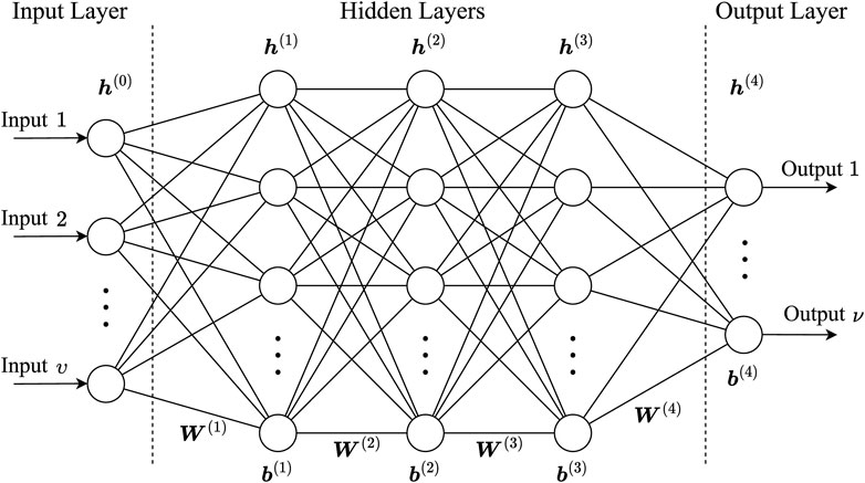
Figure 1. Example of neural network architecture.
This integration of Bayesian optimization (Asante-Okyere et al., 2022) with neural network-based regression represents a significant advancement in the field of geostatistics (Ejigu et al., 2020), potentially setting a new standard for how experimental variograms are modelled. By combining sophisticated machine learning methods (Alférez et al., 2021; Chen et al., 2024) with usual geostatistical techniques, this research opens up new avenues for more precise and reliable resource estimation and spatial data analysis, crucial for the effective exploitation and management of mineral resources.
2 Material and methods
2.1 Data description
The first step in our methodology involved the collection and preprocessing of spatial data (Bai and Tahmasebi, 2021) relevant to experimental variogram modelling (Pesquer et al., 2011). For this study, we obtained data from four orebodies characterized by similar genetic aspects (geological background). These orebodies were chosen to ensure consistency in the spatial characteristics of the data (Li Z. et al., 2018), facilitating meaningful comparisons in our analysis. The spatial data included measurements of ore grades at various locations within each orebody (Liu et al., 2022). These measurements were used to compute experimental variograms (Pardo-Igúzquiza and Dowd, 2001), which quantify the spatial dependence between pairs of data points (Fouedjio, 2016). To warrant the data reliability and accuracy, we performed careful quality control processes, including outlier detection and data cleaning. The used dataset in this research includes a medium-sized database containing 243,808 composite samples from four orebodies, all sharing the same geological characteristics (McCormick and Heaven, 2023) as the misinformed orebody, extracted from 477 drillholes. The assays encompass 16 variables, including sample coordinates (northing, easting, and elevation), ore grades and sample length. Sampling was performed at both regular and irregular intervals, with composite data at a 5 m sampling interval (Figure 2).
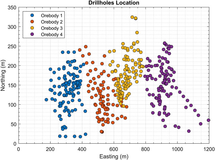
Figure 2. Drillholes spatial location.
2.2 Experimental variogram modelling
Once the spatial data were collected and preprocessed, we proceeded to model experimental variograms (Pardo-Igúzquiza et al., 2013) for each orebody. Experimental variograms were computed using the traditional method of pairwise differences, where the variance of the differences between data points, at different distances is calculated (Rivoirard, 2007). This procedure grants helpful perceptions into the data spatial structure and variability, which are fundamental for successive predictive modeling (Niu et al., 2024). It’s essentially half the anticipated square deviation among pair off random functions (Lui et al., 2022),
To compute experimental variograms, we followed standard procedures outlined in the geostatistics literature (Atkinson and Lloyd, 2007). Specifically, we calculated the semivariance between pairs of data points at various lag distances, using a predefined lag tolerance to ensure enough data pairs for reliable estimation (Afeni et al., 2021). The resulting experimental variograms were then plotted and analyzed to identify spatial trends and patterns. Instead of continuous variables, the “experimental semi-variance” stays described as quasi of the mean square off variation among quantities that are a certain lag
A mathematical model can be applied to the variogram, and its coefficients can find the best weights for spatial prediction through Kriging. The model must be conditionally negative semi-definite, as emphasized by (Atkinson and Lloyd, 2007). Typically, the model is selected from a set of approved or valid models that meet this criterion, as discussed in a review by (Li Z. et al., 2018) of commonly used valid models as spherical model Equation 3 (
2.3 Neural network regression
With the experimental variograms computed, we proceeded to develop neural network regressors (Li X. et al., 2018) for predicting variogram based on input data using conceived MATLAB scripts. Neural networks are impressive machine learning models (Friedman, 2001; Manouchehrian et al., 2012) able of catching complex relationships in data (LeCun et al., 2015), through interconnected layers of neurons. In our case, we used feedforward neural networks (Nwaila et al., 2024), which involve of an interconnected layers divided into three input layers, one or many hidden layers, and one output layeryperparameters to evalua Figure 1.
The architecture of the neural network regressors (Heaton, 2018) was carefully designed to optimize predictive performance while minimizing computational complexity (Lozano et al., 2011; Adeniran et al., 2019; Lundberg et al., 2020). We tested with many configurations, counting different numbers of hidden layers, activation functions, neurons per layer, and regularization techniques (Kim et al., 2023). These configurations were chosen based on practical evidence and domain expertise to confirm the neural networks efficiency in experimental variogram modelling.
2.4 Bayesian optimization
To fine-tune the hyperparameters (Ystroem et al., 2023) of the neural network regressor, we engaged Bayesian optimization (Zhang et al., 2020), an overwhelming optimization method that powers probabilistic models to guide the quest for optimal hyperparameters (Asante-Okyere et al., 2022). Bayesian optimization runs iteratively, operating previous valuations to update its probabilistic model and select the next set of hyperparameters to evaluate (Xie et al., 2022; Rong et al., 2023).
In our implementation of Bayesian optimization (Shahriari et al., 2016), we used Gaussian process regression (Arabpour et al., 2019; Phelps and Cronkite-Ratcliff, 2023) to model the objective function, which in this case was the performance of the neural network regressor in predicting experimental variogram. We defined appropriate acquisition functions (Zhang et al., 2020; Hallam et al., 2022), such as expected improvement or probability of improvement, to guide the search for optimal hyperparameters efficiently.
2.5 Model evaluation
To evaluate the performance of the Bayesian-optimized and the others neural network regressors, we conducted rigorous validation experiments using a holdout dataset (Adeniran et al., 2019). The dataset was randomly split into training and validation groups, ensuring that each set comprised a representative data sample (Guo et al., 2022).
The neural network regressors were trained on the training set using the best hyperparameters achieved among Bayesian optimization (Zhang et al., 2021). The accomplished models were afterward, evaluated on the validation set, using proper performance metrics (Wu and Zhou, 1993), like: Mean squared error (MSE), Coefficient of determination (R2), Mean absolute error (MAE).
2.6 Comparative analysis
Finally, we conducted a comparative analysis (Soltanmohammadi and Faroughi, 2023) to assess the performance of the Bayesian-optimized neural network regressor against non-optimized configurations (Pavlov et al., 2024). We compared the predictive accuracy of Bayesian-optimized neural network regressor with wide, bilayer, and tri-layer networks (Lauzon and Marcotte, 2022; Kim et al., 2023).
The comparative assessment engaged quantitative valuation of the performance metrics (Li Z. et al., 2018; Liu et al., 2022), as well as qualitative assessment of the predictive models accuracy and robustness (Dutta et al., 2010). By comparison of different models performance, we aimed to prove the lead of Bayesian-optimized neural network regressor (Fasnacht et al., 2020; Houshmand et al., 2022; Costa et al., 2023) in experimental variogram modelling.
3 Results
3.1 Geostatistical assessment
Statistical assessment of the composites (Pardo-Igúzquiza et al., 2013) indicated a notably low difference in ore grades, with a mean of 0.44% and a standard deviation of 0.76%. However, the coefficient of variation exceeded one. To ease training of the artificial neural network (ANN) (Hu and Shu, 2015), the data was normalized using log transformation. Figure 3 illustrates histograms of normalized and clustered data for grades of four deposits. Chart inspection of the histograms indicates that the data predominantly consists of medium-grade values, with only a small percentage of very high-grade across all deposits Figure 3.

Figure 3. Histograms of orebodies grade.
Following data analysis, we investigated spatial continuity by creating variogram models (Phelps and Cronkite-Ratcliff, 2023). Both omni-directional and directional variograms and are crucial in spatial analyses (Shi and Wang, 2021). However, in our case, we focused on constructing a downhole variogram for each orebody, using a conceived macro in Datamine Studio RM and Supervisor. The dominant direction for each orebody was found, and it was found that the four obtained directions were nearly identical due to the shared genetic context. The spatial structures (Mueller et al., 2020; Souza et al., 2023), as depicted in Figure 4, showed substantial impacts from the nugget effect, implying challenging conditions for variogram modelling (Das et al., 2020).
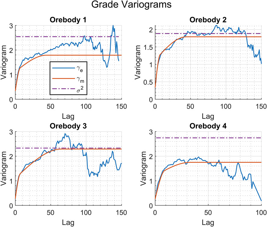
Figure 4. Experimental variograms
The obtained variogram models offered improved insight into the deposit, helping in model fitting (de Carvalho and da Costa, 2021). Figure 4 displays the downhole variogram models fitted using a spherical model. A significant portion of the spatial irregularity arising from the nugget effect suggests a medium spatial correlation structure across the study area, as indicated by the variogram plot, demonstrating good spatial correlation (Sharifzadeh Lari et al., 2021).
3.2 Detailed comparison of neural network models for experimental variogram modelling
Experimental variogram modelling is a crucial aspect of geostatistics (Allotey and Harel, 2023), providing insights into the spatial dependence (Fouedjio, 2016) of ore grades within mining environments. In this study, we evaluated four different neural network models for their effectiveness in predicting experimental variograms based on spatial data from multiple orebodies. Here, we provide a complete comparison of assessed models founded on many characteristics and performance metrics Table 1.
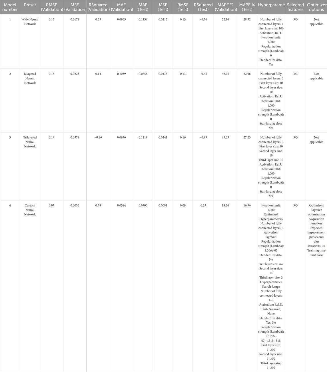
Table 1. Summary results table of the trained Neural Networks.
The wide neural network (Model 1) (He et al., 2015), with a single fully connected layer comprising 100 neurons and ReLU activation, exhibits moderate performance in experimental variogram modelling. On the validation dataset, it gets an R2 of 0.3294 and an RMSE of 0.1318, then proving an adequate data fit. Nevertheless, it is performing on the test dataset is relatively lower, with an RMSE of 0.1461 and a negative R2 of −0.7646, advocating overfitting or inadequacy in capturing the principal spatial relationships. Additionally, the model’s Mean Absolute Percentage Error for both validation (52.1646%) and test (28.5176%) datasets show an important discrepancy between predicted and actual values. The absence of regularization in this model may contribute to its susceptibility to overfitting, particularly given the limited architecture complexity Figure 5A.
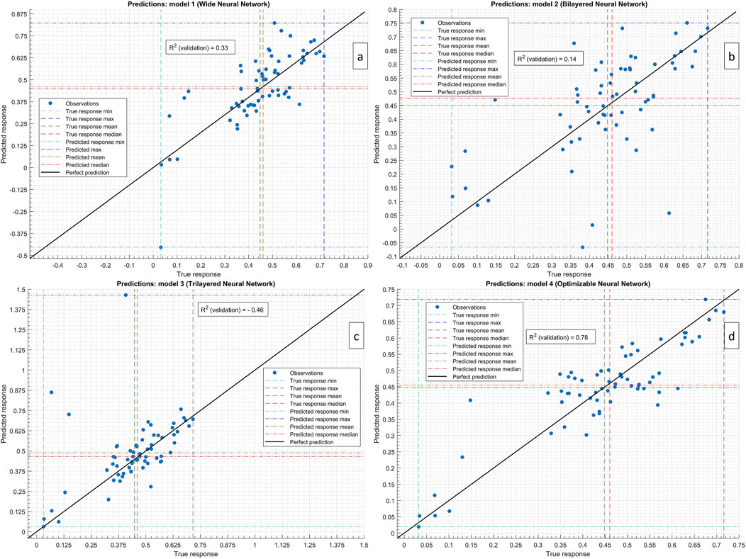
Figure 5. True response vs. Predicted response of the used Neural Networks during validation.
The bilayered neural network (Model 2), featuring two fully connected layers with 10 neurons each and ReLU activation (He et al., 2015), demonstrates slightly inferior performance compared to the wide neural network. Though it reaches the same RMSE on the validation dataset (0.1492), its R2 value is remarkably lower (0.1400), suggesting weaker predictive capability. On the test dataset, however, the bilayered network outperforms the wide network with a lower RMSE (0.1323) and a less negative R-squared value (−0.4468). This suggests that the bilayered architecture may generalize better to unseen data despite its simpler structure. The MAPE values for both validation (42.9603%) and test (22.9784%) datasets remain high, indicating notable prediction errors (Kim et al., 2023) Figure 5B.
The trilayered neural network (Model 3), featuring three fully connected layers with 10 neurons each and ReLU activation, exhibits the weakest performance among the neural network models evaluated. It attains the greatest RMSE on both validation (0.1945) and test (0.1553) datasets, revealing the smallest accurate predictions. The negative R2 values on both datasets (−0.4603 on validation, −0.9939 on test) further signify poor model fit. Additionally, the high MAPE values for both validation (45.0308%) and test (27.2294%) datasets highlight substantial discrepancies between predicted and actual values. The trilayered architecture’s increased complexity does not translate to improved performance, suggesting potential issues with model capacity or training convergence (Figure 5C).
The custom neural network (Model 4), optimized through Bayesian optimization (Figure 5D), emerges as the top-performing model for experimental variogram modelling. It achieves the least RMSE on validation and test datasets, 0.0749 and 0.0898, indicating superior predictive accuracy. With three fully connected layers, sigmoid activation, and optimized layer sizes (267, 14, and 3 neurons), Likewise, the model presents a high R2 on the validation dataset (0.7836), signifying a strong fit to the data. On the test dataset, although the R2 of 0.3335 is lower, it stays positive, implying satisfactory model performance. The MAPE values for both validation (18.2583%) and test (16.9594%) datasets are significantly lower than those of other models, indicating improved prediction accuracy and reduced errors. The absence of data standardization in this model suggests that it effectively handles the input data without requiring normalization, further simplifying the modelling process Figure 6.
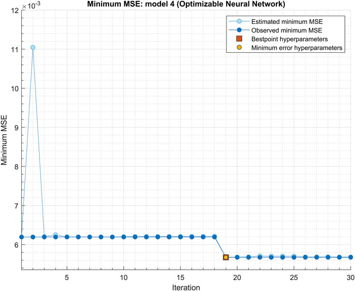
Figure 6. Minimum classification error plot of the Optimizable Neural Network (model 4).
In summary, the custom neural network (Model 4) outperforms the wide, bilayered, and trilayered neural network models in experimental variogram modelling. Its greater performance is ascribed to the hyperparameters optimization through Bayesian optimization, resulting in an architecture that effectively captures the underlying spatial patterns in the data. Compared to the other models, the custom neural network demonstrates higher predictive accuracy, stronger model fit, and reduced prediction errors, making it the preferred choice for experimental variogram modelling in mining applications.
4 Discussion
4.1 Inferences, limits, and future directions in AI-driven experimental variogram modelling
Whereas, the study investigates the use of optimized artificial neural networks models, through Bayesian optimization, for experimental variogram modelling in geostatistics, which discussion can cover an investigation of the results, inferences, limits, and future directions of the research.
4.1.1 Effectiveness of neural network models
The results demonstrate that neural network models, particularly the custom configuration optimized through Bayesian optimization, offer promising performance in experimental variogram modelling. Compared to traditional variogram modelling techniques and other neural network configurations, the custom neural network exhibits superior predictive accuracy and model fit. This underscores the potential of machine learning approaches, specifically neural networks, in capturing the complex spatial dependencies inherent in mining datasets.
4.1.2 Bayesian optimization benefits
The employment of Bayesian optimization is confirmed to be a key factor in improving the performance of neural network models for experimental variogram modelling. By systematically exploring the hyperparameter space and leveraging probabilistic models to guide the search for optimal configurations, Bayesian optimization facilitates the identification of architectures that effectively capture spatial patterns. This automated optimization process not only improves predictive accuracy but also streamlines model development, reducing the need for manual tuning and iteration.
4.1.3 Geostatistics and implications
The results of this study have major implications for geostatistical assessment, by using innovative machine learning methods, such as neural networks and Bayesian optimization, mining companies can improve their comprehension of spatial heterogeneity in ore grades. Accurate experimental variogram modelling enables more informed decision-making in resource estimation, mine planning, and optimization, ultimately leading to improved operational efficiency and profitability.
4.1.4 Limitations and challenges
Although the encouraging results, numerous limitations and challenges should be acknowledged. The computational complexity of neural network models, especially when optimized through Bayesian optimization, may present challenges for execution in resource-constrained situations. Additionally, the dependence on historical data for model training may introduce prejudices or errors, underlining the importance of data quality and typicality in geostatistical modelling.
4.1.5 Future directions
Future research directions could focus on addressing the limitations identified in this study and further refining neural network models for experimental variogram modelling. This may imply searching another optimization algorithms, such as genetic algorithms or reinforcement learning, to enhance model performance and efficiency. Also, adding other features, like geology, can enhance the model’s strength and generalization capabilities.
5 Conclusion
In this study, we have investigated the use of advanced machine learning techniques, explicitly neural networks optimized through Bayesian optimization, for experimental variogram modelling in geostatistics. Through a comprehensive analysis of four different neural network configurations and traditional experimental variogram modelling techniques, we have demonstrated the effectiveness of the custom neural network architecture in capturing the complex spatial dependencies inherent in mining datasets. The results highlight the superior predictive accuracy, model fitness, and reduced prediction errors achieved by the custom neural network, underscoring the significance of optimization methodologies in enhancing model performance.
Our results promote the extending body of work at the intersection of geostatistics and machine learning, displaying the potential of data-driven advances in attending complicated spatial challenges in mining and resource management. By utilizing sophisticated machine learning methods, mining companies can get deeper understandings into the spatial heterogeneity of ore grades, conducting to more informed decision-making in resource estimation, mine planning, and optimization. The approval of neural network models optimized through Bayesian optimization offers a hopeful avenue for refining the efficiency and accuracy of experimental variogram modelling, eventually driving operational efficiency and profitability in mining operations.
However, this study gives valued perceptions into the use of machine learning techniques for experimental variogram modelling, various openings for imminent research occur. Further searching of another optimization algorithms and model architectures can boost the robustness and generalization of the model’s capabilities. Also, the incorporation of supplementary informations, such as geology, geophysical or remote sensing data, might provide additional background and increase the accuracy of predictive models. Generally, this work places the foundation for future research intended at progressing the usage of machine learning in geostatistical analysis and mining applications, eventually contributing to sustainable resource managing and environmental custodianship in the mining industry.
Data availability statement
The raw data supporting the conclusions of this article will be made available by the authors, without undue reservation.
Author contributions
SS: Conceptualization, Data curation, Formal Analysis, Funding acquisition, Investigation, Methodology, Project administration, Software, Resources, Supervision, Validation, Visualization, Writing - original draft, Writing - review and editing. AS: Conceptualization, Data curation, Formal Analysis, Funding acquisition, Investigation, Methodology, Project administration, Resources, Software, Supervision, Validation, Visualization, Writing–original draft, Writing–review and editing. KA: Conceptualization, Data curation, Formal Analysis, Funding acquisition, Investigation, Methodology, Project administration, Resources, Software, Supervision, Validation, Visualization, Writing–original draft, Writing–review and editing. AM: Conceptualization, Data curation, Formal Analysis, Funding acquisition, Investigation, Methodology, Project administration, Resources, Software, Supervision, Validation, Visualization, Writing–review and editing, Writing–original draft. MF: Conceptualization, Data curation, Formal Analysis, Funding acquisition, Investigation, Methodology, Project administration, Resources, Software, Supervision, Validation, Visualization, Writing–review and editing. BM: Conceptualization, Data curation, Formal Analysis, Funding acquisition, Investigation, Methodology, Project administration, Resources, Software, Supervision, Validation, Visualization, Writing–review and editing.
Funding
The author(s) declare that financial support was received for the research, authorship, and/or publication of this article. This research was funded by the Researchers Supporting Project Number (RSP2024R249), King Saud University, Riyadh, Saudi Arabia.
Acknowledgments
We would like to thank MathWorks and Datamine software for their assistance during the development of the work. Deep thanks and gratitude to the Researchers Supporting Project Number (RSP2024R249), King Saud University, Riyadh, Saudi Arabia, for funding this research article.
Conflict of interest
The authors declare that the research was conducted in the absence of any commercial or financial relationships that could be construed as a potential conflict of interest.
Publisher’s note
All claims expressed in this article are solely those of the authors and do not necessarily represent those of their affiliated organizations, or those of the publisher, the editors and the reviewers. Any product that may be evaluated in this article, or claim that may be made by its manufacturer, is not guaranteed or endorsed by the publisher.
References
Abildin, Y., Xu, C., Dowd, P., and Adeli, A. (2022). A hybrid framework for modelling domains using quantitative covariates. Appl. Comput. Geosci. 16, 100107. doi:10.1016/j.acags.2022.100107
Adeniran, A. A., Adebayo, A. R., Salami, H. O., Yahaya, M. O., and Abdulraheem, A. (2019). A competitive ensemble model for permeability prediction in heterogeneous oil and gas reservoirs. Appl. Comput. Geosci. 1, 100004. doi:10.1016/j.acags.2019.100004
Afeni, T. B., Akeju, V. O., and Aladejare, A. E. (2021). A comparative study of geometric and geostatistical methods for qualitative reserve estimation of limestone deposit. Geosci. Front. 12, 243–253. doi:10.1016/j.gsf.2020.02.019
Alférez, G. H., Vázquez, E. L., Martínez Ardila, A. M., and Clausen, B. L. (2021). Automatic classification of plutonic rocks with deep learning. Appl. Comput. Geosci. 10, 100061. doi:10.1016/j.acags.2021.100061
Ali, M., Zhu, P., Huolin, M., Jiang, R., Zhang, H., Ashraf, U., et al. (2024a). Data-driven machine learning approaches for precise lithofacies identification in complex geological environments. Geo-Spat. Inf. Sci., 1–21. doi:10.1080/10095020.2024.2405635
Ali, M., Zhu, P., Jiang, R., Huolin, M., Ashraf, U., Zhang, H., et al. (2024b). Data-driven lithofacies prediction in complex tight sandstone reservoirs: a supervised workflow integrating clustering and classification models. Geomech. Geophys. Geo-Energy Geo-Resour. 10, 70. doi:10.1007/s40948-024-00787-5
Allotey, P. A., and Harel, O. (2023). Modeling geostatistical incomplete spatially correlated survival data with applications to COVID-19 mortality in Ghana. Spat. Stat. 54, 100730. doi:10.1016/j.spasta.2023.100730
Arabpour, A., Asghari, O., and Mirnejad, H. (2019). Supergene mass-balance study assuming zero lateral copper flux using geostatistics to recognize metal source zones in exotic copper deposits. Nat. Resour. Res. 28, 1353–1370. doi:10.1007/s11053-018-09449-2
Asante-Okyere, S., Shen, C., and Osei, H. (2022). Enhanced machine learning tree classifiers for lithology identification using Bayesian optimization. Appl. Comput. Geosci. 16, 100100. doi:10.1016/j.acags.2022.100100
Ashraf, U., Anees, A., Zhang, H., Ali, M., Thanh, H. V., and Yuan, Y. (2024a). Identifying payable cluster distributions for improved reservoir characterization: a robust unsupervised ML strategy for rock typing of depositional facies in heterogeneous rocks. Geomech. Geophys. Geo-Energy Geo-Resour. 10, 131. doi:10.1007/s40948-024-00848-9
Ashraf, U., Shi, W., Zhang, H., Anees, A., Jiang, R., Ali, M., et al. (2024b). Reservoir rock typing assessment in a coal-tight sand based heterogeneous geological formation through advanced AI methods. Sci. Rep. 14, 5659. doi:10.1038/s41598-024-55250-y
Atkinson, P. M., and Lloyd, C. D. (2007). Non-stationary variogram models for geostatistical sampling optimisation: an empirical investigation using elevation data. Comput. Geosci. 33, 1285–1300. doi:10.1016/j.cageo.2007.05.011
Bai, T., and Tahmasebi, P. (2021). Accelerating geostatistical modeling using geostatistics-informed machine Learning. Comput. Geosci. 146, 104663. doi:10.1016/j.cageo.2020.104663
Chen, Z., Yuan, F., Li, X., Zhang, M., and Zheng, C. (2024). A novel few-shot learning framework for rock images dually driven by data and knowledge. Appl. Comput. Geosci. 21, 100155. doi:10.1016/j.acags.2024.100155
Costa, F. R., Carneiro, C. de C., and Ulsen, C. (2023). Imputation of gold recovery data from low grade gold ore using artificial neural network. Minerals 13, 340. doi:10.3390/min13030340
Das, P. P., Mohapatra, P. P., Goswami, S., Mishra, M., and Pattanaik, J. K. (2020). A geospatial investigation of interlinkage between basement fault architecture and coastal aquifer hydrogeochemistry. Geosci. Front. 11, 1431–1440. doi:10.1016/j.gsf.2019.12.008
de Carvalho, P. R. M., and da Costa, J. F. C. L. (2021). Automatic variogram model fitting of a variogram map based on the Fourier integral method. Comput. Geosci. 156, 104891. doi:10.1016/j.cageo.2021.104891
Djimadoumngar, K.-N. (2023). Parallel investigations of remote sensing and ground-truth Lake Chad’s level data using statistical and machine learning methods. Appl. Comput. Geosci. 20, 100135. doi:10.1016/j.acags.2023.100135
Dutta, S., Bandopadhyay, S., Ganguli, R., and Misra, D. (2010). Machine learning algorithms and their application to ore reserve estimation of sparse and imprecise data. J. Intell. Learn. Syst. Appl. 02, 86–96. doi:10.4236/jilsa.2010.22012
Ejigu, B. A., Wencheko, E., Moraga, P., and Giorgi, E. (2020). Geostatistical methods for modelling non-stationary patterns in disease risk. Spat. Stat. 35, 100397. doi:10.1016/j.spasta.2019.100397
Fasnacht, L., Renard, P., and Brunner, P. (2020). Robust input layer for neural networks for hyperspectral classification of data with missing bands. Appl. Comput. Geosci. 8, 100034. doi:10.1016/j.acags.2020.100034
Fouedjio, F. (2016). A hierarchical clustering method for multivariate geostatistical data. Spat. Stat. 18, 333–351. doi:10.1016/j.spasta.2016.07.003
Friedman, J. H. (2001). Greedy function approximation: a gradient boosting machine. Ann. Stat. 29, 1189–1232. doi:10.1214/aos/1013203451
Fronterrè, C., Giorgi, E., and Diggle, P. (2018). Geostatistical inference in the presence of geomasking: a composite-likelihood approach. Spat. Stat. 28, 319–330. doi:10.1016/j.spasta.2018.06.004
Guo, J., Wang, Z., Li, C., Li, F., Jessell, M. W., Wu, L., et al. (2022). Multiple-point geostatistics-based three-dimensional automatic geological modeling and uncertainty analysis for borehole data. Nat. Resour. Res. 31, 2347–2367. doi:10.1007/s11053-022-10071-6
Hallam, A., Mukherjee, D., and Chassagne, R. (2022). Multivariate imputation via chained equations for elastic well log imputation and prediction. Appl. Comput. Geosci. 14, 100083. doi:10.1016/j.acags.2022.100083
He, K., Zhang, X., Ren, S., and Sun, J. (2015). “Delving deep into rectifiers: surpassing human-level performance on imagenet classification,” in Proceedings of the IEEE international conference on computer vision (IEEE), 1026–1034. doi:10.1109/ICCV.2015.123
Heaton, J. (2018). Ian goodfellow, yoshua bengio, and aaron courville: deep learning. Genet. Program. Evolvable Mach. 19, 305–307. doi:10.1007/s10710-017-9314-z
Hooten, M. B., Schwob, M. R., Johnson, D. S., and Ivan, J. S. (2024). Geostatistical capture–recapture models. Spat. Stat. 59, 100817. doi:10.1016/j.spasta.2024.100817
Houshmand, N., GoodFellow, S., Esmaeili, K., and Ordóñez Calderón, J. C. (2022). Rock type classification based on petrophysical, geochemical, and core imaging data using machine and deep learning techniques. Appl. Comput. Geosci. 16, 100104. doi:10.1016/j.acags.2022.100104
Hu, H., and Shu, H. (2015). An improved coarse-grained parallel algorithm for computational acceleration of ordinary Kriging interpolation. Comput. Geosci. 78, 44–52. doi:10.1016/J.CAGEO.2015.02.011
Kim, S., Hong, Y., Lim, J. T., and Kim, K. H. (2023). Improved prediction of shale gas productivity in the Marcellus shale using geostatistically generated well-log data and ensemble machine learning. Comput. Geosci. 181, 105452. doi:10.1016/j.cageo.2023.105452
Lauzon, D., and Marcotte, D. (2022). Statistical comparison of variogram-based inversion methods for conditioning to indirect data. Comput. Geosci. 160, 105032. doi:10.1016/j.cageo.2022.105032
LeCun, Y., Bengio, Y., and Hinton, G. (2015). Deep learning. Nature 521, 436–444. doi:10.1038/nature14539
Li, X., Zhang, L., and Zhang, S. (2018a). Efficient Bayesian networks for slope safety evaluation with large quantity monitoring information. Geosci. Front. 9, 1679–1687. doi:10.1016/j.gsf.2017.09.009
Li, Z., Zhang, X., Clarke, K. C., Liu, G., and Zhu, R. (2018b). An automatic variogram modeling method with high reliability fitness and estimates. Comput. Geosci. 120, 48–59. doi:10.1016/j.cageo.2018.07.011
Liao, Z., Zhu, P., Zhang, H., Li, Z., Li, Z., and Ali, M. (2024). A deep learning-based seismic horizon tracking method with uncertainty encoding and vertical constraint. IEEE Trans. Geosci. Remote Sens. 62, 1–13. doi:10.1109/TGRS.2024.3424467
Liu, G., Fang, H., Chen, Q., Cui, Z., and Zeng, M. (2022). A feature-enhanced mps approach to reconstruct 3D deposit models using 2D geological cross sections: a case study in the luodang Cu deposit, southwestern China. Nat. Resour. Res. 31, 3101–3120. doi:10.1007/s11053-022-10113-z
Lozano, A. C., Świrszcz, G., and Abe, N. (2011). Group orthogonal matching pursuit for logistic regression. J. Mach. Learn. Res. 15, 452–460.
Lui, T. C. C., Gregory, D. D., Anderson, M., Lee, W.-S., and Cowling, S. A. (2022). Applying machine learning methods to predict geology using soil sample geochemistry. Appl. Comput. Geosci. 16, 100094. doi:10.1016/j.acags.2022.100094
Lundberg, S. M., Erion, G., Chen, H., DeGrave, A., Prutkin, J. M., Nair, B., et al. (2020). From local explanations to global understanding with explainable AI for trees. Nat. Mach. Intell. 2, 56–67. doi:10.1038/s42256-019-0138-9
Manouchehrian, A., Sharifzadeh, M., and Moghadam, R. H. (2012). Application of artificial neural networks and multivariate statistics to estimate UCS using textural characteristics. Int. J. Min. Sci. Technol. 22, 229–236. doi:10.1016/j.ijmst.2011.08.013
McCormick, T., and Heaven, R. E. (2023). The British Geological Survey Rock Classification Scheme, its representation as linked data, and a comparison with some other lithology vocabularies. Appl. Comput. Geosci. 20, 100140. doi:10.1016/j.acags.2023.100140
Mueller, U., Tolosana Delgado, R., Grunsky, E. C., and McKinley, J. M. (2020). Biplots for compositional data derived from generalized joint diagonalization methods. Appl. Comput. Geosci. 8, 100044. doi:10.1016/j.acags.2020.100044
Nakamura, K. (2023). A practical approach for discriminating tectonic settings of basaltic rocks using machine learning. Appl. Comput. Geosci. 19, 100132. doi:10.1016/j.acags.2023.100132
Niu, Y., Lindsay, M., Coghill, P., Scalzo, R., and Zhang, L. (2024). A Bayesian hierarchical model for the inference between metal grade with reduced variance: case studies in porphyry Cu deposits. Geosci. Front. 15, 101767. doi:10.1016/j.gsf.2023.101767
Nwaila, G. T., Zhang, S. E., Bourdeau, J. E., Frimmel, H. E., and Ghorbani, Y. (2024). Spatial interpolation using machine learning: from patterns and regularities to block models. Springer US. doi:10.1007/s11053-023-10280-7
Pardo-Igúzquiza, E., and Dowd, P. A. (2001). VARIOG2D: a computer program for estimating the semi-variogram and its uncertainty. Comput. Geosci. 27, 549–561. doi:10.1016/S0098-3004(00)00165-5
Pardo-Igúzquiza, E., Dowd, P. A., Baltuille, J. M., and Chica-Olmo, M. (2013). Geostatistical modelling of a coal seam for resource risk assessment. Int. J. Coal Geol. 112, 134–140. doi:10.1016/j.coal.2012.11.004
Pavlov, M., Peshkov, G., Katterbauer, K., and Alshehri, A. (2024). Geosteering based on resistivity data and evolutionary optimization algorithm. Appl. Comput. Geosci. 22, 100162. doi:10.1016/j.acags.2024.100162
Pesquer, L., Cortés, A., and Pons, X. (2011). Parallel ordinary kriging interpolation incorporating automatic variogram fitting. Comput. Geosci. 37, 464–473. doi:10.1016/j.cageo.2010.10.010
Phelps, G. A., and Cronkite-Ratcliff, C. (2023). Near surface sediments introduce low frequency noise into gravity models. Appl. Comput. Geosci. 19, 100131. doi:10.1016/j.acags.2023.100131
Rivoirard, J. (2007). Concepts and methods of geostatistics. Space Struct. Randomness, 17–37. doi:10.1007/0-387-29115-6_2
Rong, G., Li, K., Tong, Z., Liu, X., Zhang, J., Zhang, Y., et al. (2023). Population amount risk assessment of extreme precipitation-induced landslides based on integrated machine learning model and scenario simulation. Geosci. Front. 14, 101541. doi:10.1016/j.gsf.2023.101541
Saikia, K., and Sarkar, B. C. (2013). Coal exploration modelling using geostatistics in Jharia coalfield, India. Int. J. Coal Geol. 112, 36–52. doi:10.1016/j.coal.2012.11.012
Shahriari, B., Swersky, K., Wang, Z., Adams, R. P., and de Freitas, N. (2016). Taking the human out of the loop: a review of bayesian optimization. Proc. IEEE 104, 148–175. doi:10.1109/JPROC.2015.2494218
Sharifzadeh Lari, M., Straubhaar, J., and Renard, P. (2021). Efficiency of template matching methods for Multiple-Point Statistics simulations. Appl. Comput. Geosci. 11, 100064. doi:10.1016/j.acags.2021.100064
Shi, C., and Wang, Y. (2021). Non-parametric machine learning methods for interpolation of spatially varying non-stationary and non-Gaussian geotechnical properties. Geosci. Front. 12, 339–350. doi:10.1016/j.gsf.2020.01.011
Soltanmohammadi, R., and Faroughi, S. A. (2023). A comparative analysis of super-resolution techniques for enhancing micro-CT images of carbonate rocks. Appl. Comput. Geosci. 20, 100143. doi:10.1016/j.acags.2023.100143
Souza, J. P. P., Matheus, G. F., Basso, M., Chinelatto, G. F., and Vidal, A. C. (2023). Generation of μCT images from medical CT scans of carbonate rocks using a diffusion-based model. Appl. Comput. Geosci. 18, 100117. doi:10.1016/j.acags.2023.100117
Tilahun, T., and Korus, J. (2023). 3D hydrostratigraphic and hydraulic conductivity modelling using supervised machine learning. Appl. Comput. Geosci. 19, 100122. doi:10.1016/j.acags.2023.100122
Valakas, G., Seferli, M., and Modis, K. (2023). Co-simulation of hydrofacies and piezometric data in the West Thessaly basin, Greece: a geostatistical application using the GeoSim R package. Appl. Comput. Geosci. 20, 100139. doi:10.1016/j.acags.2023.100139
Wu, X., and Zhou, Y. (1993). Reserve estimation using neural network techniques. Comput. Geosci. 19, 567–575. doi:10.1016/0098-3004(93)90082-G
Xie, C., Nguyen, H., Choi, Y., and Jahed Armaghani, D. (2022). Optimized functional linked neural network for predicting diaphragm wall deflection induced by braced excavations in clays. Geosci. Front. 13, 101313. doi:10.1016/j.gsf.2021.101313
Ystroem, L. H., Vollmer, M., Kohl, T., and Nitschke, F. (2023). AnnRG - an artificial neural network solute geothermometer. Appl. Comput. Geosci. 20, 100144. doi:10.1016/j.acags.2023.100144
Zhang, H., Song, X., Zhu, P., Ali, M., Liao, Z., Ruan, D., et al. (2024). A two-stage convolutional neural network for interactive channel segmentation from 3-D seismic data. IEEE Trans. Geosci. Remote Sens. 62, 1–15. doi:10.1109/TGRS.2024.3401867
Zhang, W., Wu, C., Zhong, H., Li, Y., and Wang, L. (2021). Prediction of undrained shear strength using extreme gradient boosting and random forest based on Bayesian optimization. Geosci. Front. 12, 469–477. doi:10.1016/j.gsf.2020.03.007
Keywords: geostatistics, experimental variogram, machine learning, neural network, Bayesian optimization
Citation: Soulaimani S, Soulaimani A, Abdelrahman K, Miftah A, Fnais MS and Mondal BK (2024) Geostatistics and artificial intelligence coupling: advanced machine learning neural network regressor for experimental variogram modelling using Bayesian optimization. Front. Earth Sci. 12:1474586. doi: 10.3389/feart.2024.1474586
Received: 01 August 2024; Accepted: 27 November 2024;
Published: 12 December 2024.
Edited by:
Umar Ashraf, Yunnan University, ChinaReviewed by:
Muhammad Ali, Chinese Academy of Sciences (CAS), ChinaVasily Golubev, Moscow Institute of Physics and Technology, Russia
Copyright © 2024 Soulaimani, Soulaimani, Abdelrahman, Miftah, Fnais and Mondal. This is an open-access article distributed under the terms of the Creative Commons Attribution License (CC BY). The use, distribution or reproduction in other forums is permitted, provided the original author(s) and the copyright owner(s) are credited and that the original publication in this journal is cited, in accordance with accepted academic practice. No use, distribution or reproduction is permitted which does not comply with these terms.
*Correspondence: Saâd Soulaimani, c291bGFpbWFuaUBlbmltLmFjLm1h; Kamal Abdelrahman, a2hhc3NhbmVpbkBrc3UuZWR1LnNh; Abdelhalim Miftah, YS5taWZ0YWhAdWhwLmFjLm1h