Estimation of the depth-variant seismic wavelet based on the modified unscaled S-transform

Seismic inversion is one of the key techniques used for reservoir characterization. Depth-domain seismic inversion eliminates the cumulative errors associated with depth-to-time and time-to-depth conversions, thus providing geologists and reservoir engineers with an intuitive basis for geological interpretation. The method has received increasing attention in the field of reservoir characterization. Extracting accurate depth-domain seismic wavelets is a prerequisite for successful depth-domain seismic inversion. However, the depth-domain wavelet is velocity-dependent and exhibits significant non-stationarity, which leads to the failure of seismic wavelet estimation methods based on the stationary convolutional model. To this end, we propose a modified wavenumber-domain unscaled S-transform (MWUST) method to accomplish accurate estimation of depth-domain seismic wavelets. The proposed method enhances the accuracy of wavenumber components by removing the linear wavenumber-dependent term from the S-transform. Furthermore, it introduces slope and intercept parameters to improve the depth resolution at low wavenumbers, thereby yielding a more reliable depth–wavenumber spectrum. Subsequently, the relationship between the non-stationary depth-domain seismic wavelet and the depth–wavenumber spectrum is established, allowing for the accurate extraction of non-stationary wavelets under the assumption that the depth-domain reflectivity is a random sequence. Synthetic and real data applications have been used to verify the effectiveness of the proposed method.

1 Introduction

With continuous advancements in oil and gas exploration, the demands for accurate reservoir characterization are becoming increasingly stringent. Seismic inversion is a key technique used for obtaining elastic parameters for reservoir characterization (Zhang et al., 2021b; Zhou et al., 2021; Wang P. et al., 2022; Zhang et al., 2022c; Wang et al., 2024). Many depth migration methods have been developed and are widely used to generate depth-domain seismic images, leading to a growing need for depth-domain seismic inversion of subsurface elastic properties for reservoir characterization (Li et al., 2020; Li et al., 2022; Paxton et al., 2022; Shadlow et al., 2022; Wang N. et al., 2022; Zhang and Deng, 2023). Depth-domain seismic inversion avoids the cumulative errors associated with depth-to-time and time-to-depth conversions, providing geologically significant results for geologists and reservoir engineers. However, depth-domain seismic inversion is different from time-domain seismic inversion, in that methods applicable in the time domain cannot be directly applied to the depth domain. The primary difference is that depth-domain seismic data exhibit strong spectral variability. This is because the depth-domain seismic wavelet depends on velocity, i.e., higher velocity results in longer waveforms, and vice versa. This makes it challenging to assume stationarity in depth-domain seismic data, which can lead to erroneous inversion results. In order to obtain reliable results, the accurate extraction of the depth-domain seismic wavelet is a prerequisite (Cai et al., 2024).

Typically, seismic wavelets can be estimated by statistical and deterministic approaches (Zhang et al., 2022a). Statistical methods estimate seismic wavelets using only seismic data (Lazear, 1993; Walden and White, 1998; Sacchi and Ulrych, 2000; van der Baan, 2008; Sengupta et al., 2018; Zhang and Deng, 2018; Laake et al., 2019), whereas deterministic methods rely on a combination of seismic and well-log data to estimate the wavelets (Danielsen and Karlsson, 1984; Lines and Treitel, 1985; Buland and Omre, 2003; Gunning and Glinsky, 2006; De Macedo and De Figueiredo, 2020; Ke et al., 2023). Given the limited well data in the field region, the time–frequency decomposition method, which is a statistical approach, serves as a suitable choice for estimating non-stationary seismic wavelets. Zhang and Deng (2018) extended the S-transform (ST)-based time–frequency decomposition method from the time–frequency domain to the depth–wavenumber domain, thereby completing the estimation of non-stationary seismic wavelets in the depth domain. Sengupta et al. (2021) successfully estimated the depth-domain seismic wavelet using the ST and used it for depth-domain pre-stack seismic inversion, thereby obtaining reliable depth-domain elastic parameters including P- and S-wave velocity and density. Zhang and Deng (2023) developed a depth–wavenumber decomposition technique that applies the ST to depth-domain pre-stack angle gathers, generating depth and angle-variant wavelets for inversion. Tang et al. (2024) introduced a generalized unscaled ST for the spectral decomposition of depth-domain seismic data, estimating seismic wavelets by utilizing local spectral information at each depth sampling point.

The spectral decomposition method entails performing depth–wavenumber spectral decomposition on depth-domain seismic data and estimating depth-variant wavelets from the resulting depth–wavenumber spectrum. As a hybrid of the short-time Fourier transform and the continuous wavelet transform, the ST combines the advantages of both, offering adaptive resolution adjustment and lossless reversible transformation. The generalized S-transform (GST) was later developed for specific applications. However, the linear frequency-dependent term in the ST or GST causes its frequency distribution to deviate from the true values. This leads to incorrect estimation of seismic wavelets, which affects the accuracy of the subsequent depth-domain seismic inversion. Wu and Castagna (2017) developed an unscaled ST (UST) algorithm to reduce the bias in frequency components by removing the linear frequency-dependent term of the ST. Wang (2016) derived the frequency domain form of the UST that preserves the signal amplitude. However, the removal of the linear frequency-dependent term reduces their temporal resolution at low frequencies. Li et al. (2016) introduced slope and intercept parameters into the generalized ST to achieve the desired time–frequency resolution. Zhang et al. (2022b) further improved the temporal resolution of the time–frequency spectrum by modifying the basis in the study by Wu and Castagna (2017), while ensuring the preservation of frequency characteristics. Existing wavelet extraction methods based on spectral decomposition are constrained by the limitations of the spectral decomposition algorithm, which reduces the accuracy of wavelet extraction. Inspired by this, we combine the advantages of the aforementioned time–frequency decomposition methods to re-derive a modified frequency-domain unscaled ST algorithm and extend it to the wavenumber domain (MWUST), thereby achieving an accurate estimation of non-stationary seismic wavelets in the depth domain. The effectiveness of the proposed method is verified through a series of numerical experiments and by comparison with traditional ST (Zhang and Deng, 2018)- and UST (Tang et al., 2024)-based depth-domain wavelet extraction methods.

2 Methods

Depth-domain seismic inversion requires a reliable depth-domain seismic wavelet as a prerequisite. In order to obtain a reliable depth-domain seismic wavelet, a reliable depth–wavenumber decomposition method is required. In this section, we first derive a modified frequency-domain unscaled ST algorithm and extend it to the wavenumber domain. Then, we describe in detail the estimation of the depth-domain seismic wavelet based on the depth–wavenumber spectrum obtained through the proposed method.

2.1 The modified wavenumber-domain unscaled S transform

For a time-domain signal $x\left(t\right)$, the time–frequency spectrum $S\left(t,f\right)$ based on the ST is expressed as Equation 1 (Stockwell et al., 1996)

$S\left(\tau ,f\right)={\int }_{-\infty }^{+\infty }x\left(t\right)g\left(t-\tau ,f\right)e^{-i2\pi ft}dt,(1)$

where $g\left(t\right)$ is the Gaussian window of the specific form $\frac{\left|f\right|}{\sqrt{2\pi }}{e}^{-\frac{t^2{f}^2}{2}}$, $\tau$ is a translation factor to control the position of the Gaussian window on the time axis $t$, $f$ represents the frequency, and $i$ is imaginary units.

Then, the depth–wavenumber spectrum of a depth-domain signal based on the ST can be expressed as Equation 2

$S\left(\eta ,k\right)={\int }_{-\infty }^{+\infty }x\left(h\right)g\left(h-\eta ,k\right)e^{-i2\pi kh}dh,(2)$

where $g\left(h\right)$ represents the depth-domain Gaussian window of the specific form $\frac{\left|k\right|}{\sqrt{2\pi }}{e}^{-\frac{h^2{k}^2}{2}}$, $\eta$ is a translation factor to control the position of the Gaussian window on the depth axis $h$, and $k$ represents the wavenumber.

To reduce the bias of the frequency components in the time–frequency spectrum based on the ST, the time-domain UST removes the linear frequency-dependent term $\left|f\right|$ of $g\left(t\right)$. Then, the depth-domain UST is derived as

$S_1\left(\eta ,k\right)={\int }_{-\infty }^{+\infty }x\left(h\right)\frac{1}{\sqrt{2\pi }}{e}^{-\frac{{\left(h-\eta \right)}^2{k}^2}{2}}{e}^{-i2\pi kh}dh.(3)$

Then, the expression to the right of the equal sign in Equation 3 in the wavenumber domain (i.e., WUST) can be written as

$S_1\left(\eta ,k\right)={\int }_{-\infty }^{+\infty }X\left(\alpha +k\right)\frac{1}{\left|k\right|}{e}^{-\frac{2{\pi }^2{\alpha }^2}{k^2}}{e}^{i2\pi \alpha \eta }d\alpha ,k\ne 0,(4)$

where $X\left(\alpha +k\right)$ is the Fourier transform of $x\left(h\right)e^{-i2\pi kh}$. $\alpha$ denotes the translating wavenumber (Wang, 2016).

However, the UST sacrifices time/depth resolution at low frequencies/low wavenumbers in order to obtain a reliable frequency/wavenumber distribution. To overcome this shortcoming, slope ($A$) and intercept ($B$) parameters are introduced to obtain the desired depth–wavenumber resolution. The equation of the modified UST in the depth domain is

$S_2\left(\eta ,k\right)={\int }_{-\infty }^{+\infty }x\left(h\right)\frac{1}{\sqrt{2\pi }}{e}^{-\frac{{\left(h-\eta \right)}^2{\left(Ak+B\right)}^2}{2}}{e}^{-i2\pi kh}dh.(5)$

Based on the convolution theorem, the expression to the right of the equal sign in Equation 5 in the wavenumber domain (i.e., MWUST) can be written as

$S_2\left(\eta ,k\right)={\int }_{-\infty }^{+\infty }X\left(\alpha +k\right)\frac{1}{\left|Ak+B\right|}{e}^{-\frac{2{\pi }^2{\alpha }^2}{{\left(Ak+B\right)}^2}}{e}^{i2\pi \alpha \eta }d\alpha ,k\ne 0,(6)$

where $X\left(\alpha +k\right)$ is the Fourier transform of $x\left(h\right)e^{-i2\pi kh}$. The constant average of the signal $x\left(h\right)$ is put into zero wavenumber, which ensures the feasibility of the inverse transform. By integrating and inverse Fourier-transforming along different axes, we can reconstruct the original signal. It is worth noting that Equation 6 degenerates to Equation 4 when $A=1$ and $B=0$.

There are two parameters (i.e., A and B) in the proposed method that need to be determined in advance. For different tasks and frequencies, the values of A and B may vary, which requires manual adjustment. One can use trial-and-error methods to obtain relatively optimal results. However, before that, we can use the full-window spatial or wavenumber width at half-maximum (FWHM) to roughly estimate parameters A and B (Li et al., 2016; Zhang et al., 2022b). For the depth and wavenumber domains, there are different expressions for A and B.

For the depth domain, A and B have the following expressions (Equation 7) (George et al., 2009):

$\left\{\begin{array}{l}A=\frac{2.355\left(\frac{1}{\Delta h_2}-\frac{1}{\Delta h_1}\right)}{k_2-k_1}\\ B=\frac{2.355}{\Delta h_1}-A{k}_1\end{array}\right.,(7)$

where $∆h_1$ and $∆h_2$ represent specified spatial (or depth) FWHM resolutions at wavenumbers $k_1$ and $k_2$, respectively.

For the wavenumber domain, A and B have the following expressions (Equation 8):

$\left\{\begin{array}{l}A=\frac{2.668\left(\Delta {\alpha }_2-\Delta {\alpha }_1\right)}{k_2-k_1}\\ B=\frac{2.668\left(\Delta {\alpha }_1{k}_2-\Delta {\alpha }_2{k}_2\right)}{k_2-k_1}\end{array}\right.,(8)$

where $∆{\alpha }_1$ and $∆{\alpha }_2$ represent specified wavenumber FWHM resolutions at wavenumbers $k_1$ and $k_2$, respectively.

Figure 1 shows relationships between FWHM amplitudes and wavenumber for different A and B expressions. In Figure 1A, the width of the MWUST is narrower than that of the WUST in the low-wavenumber region when $A>1$ (i.e., orange-, green-, and gray-solid curves). It indicates that the MWUST has higher resolution in the low-wavenumber region, and the difference decreases as the wavenumber increases. When $A<1$, shown as a purple solid curve, the width of the MWUST is broader than that of the WUST in the high-wavenumber region, indicated by larger depth FWHM values. The wavenumber FWHM values increase linearly as the wavenumber increases, as shown in Figure 1B. From Figure 1, it can also be noticed that A plays a greater role for FWHM values than B, indicating that A has a great influence on the depth–wavenumber resolution. B controls the starting depth resolution.

Figure 1

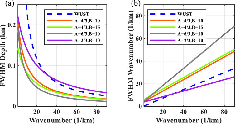
Figure 1. Full-window spatial or wavenumber width at half-maximum (FWHM) amplitudes versus wavenumber (A) in the depth domain and (B) the wavenumber domain.

2.2 Depth-domain seismic wavelet estimation based on the depth–wavenumber spectrum

The depth-domain non-stationary convolution model is expressed as

$u\left(x\right)={\int }_{-\infty }^{+\infty }w\left(x-\eta ,\eta \right)r\left(\eta \right)d\eta ,(9)$

where $u\left(x\right)$ represents depth-domain synthetic seismic records, $w\left(x,\eta \right)$ represents the non-stationary depth-domain seismic wavelet, and $r\left(\eta \right)$ represents the depth-domain reflectivity series. Equation 9 is transformed into the wavenumber domain with the following expression (Equation 10):

$U\left(k\right)={\int }_{-\infty }^{+\infty }R\left(\xi \right)W\left(k,k-\xi \right)d\xi ,(10)$

where $W\left(k,\xi \right)$ is the 2D Fourier transformation of $w\left(x,\eta \right)$. $U\left(k\right)$ and $R\left(\xi \right)$ are the Fourier transformation of $u\left(x\right)$ and $r\left(\eta \right)$, respectively. If $r$ is the random reflectivity, we have (Yilmaz, 2001)

$U\left(k\right)=R_{\xi }{\int }_{-\infty }^{+\infty }W\left(k,\xi \right)d\xi ,(11)$

where $R_{\xi }$ is a constant value, which can be determined from the well-side seismic traces. We then perform the inverse Fourier transform to Equation 11 to reproduce the original signal, as follows (Equation 12):

$u\left(x\right)={\int }_{-\infty }^{+\infty }U\left(k\right)e^{2\pi ikx}dk=R_{\xi }{\int }_{-\infty }^{+\infty }{\int }_{-\infty }^{+\infty }W\left(k,\xi \right)e^{2\pi ikx}d\xi dk=R_{\xi }{\int }_{-\infty }^{+\infty }w\left(x,\xi \right)d\xi .(12)$

Combined with the original signal reconstruction method, the following expression is obtained:

$R_{\xi }{\int }_{-\infty }^{+\infty }w\left(x,\xi \right)d\xi ={\int }_{-\infty }^{+\infty }S\left(x,\eta \right)d\eta ,(13)$

where $w\left(x,\xi \right)$ represents the depth-domain seismic wavelet and $S\left(x,\eta \right)$ represents the results after inverse Fourier transform along the depth of the depth–wavenumber spectrum (e.g., $S_2$). Then, the estimation of the depth-domain seismic wavelet can be achieved based on the depth–wavenumber spectrum calculated by the method proposed in Section 2.1.

3 Application

To validate the proposed approach, we apply it to synthetic experiments and real data. We first illustrate the differences between depth-domain and time-domain wavelets under different velocity model conditions and further apply the proposed method to the single-wavelet model. A three-wavelet model is then designed based on the single-wavelet model to verify the validity of the proposed method. Finally, well-log data are used for testing, and the extracted wavelet is used for depth-domain inversion to obtain satisfactory results.

3.1 Synthetic data test

We first experiment with the proposed method using a simple three-wavelet model, referencing the model used in Zhang and Deng (2018). Figure 2A shows a 40-Hz zero-phase time-domain Ricker wavelet, and its corresponding amplitude spectrum is shown in Figure 2B. Taking this wavelet as the source, the corresponding depth-domain wavelets as they propagate through the different velocity strata are shown in Figure 2C, and their corresponding amplitude spectrums are shown in Figure 2D. It can be seen that as the velocity changes, the depth-domain wavelet is significantly stretched or compressed, i.e., the depth-domain wavelet is velocity-dependent. Since subsurface velocities are spatially variable, the interpretation and inversion of depth-domain seismic data can result in unreliable results if a constant wavelet is utilized.

Figure 2

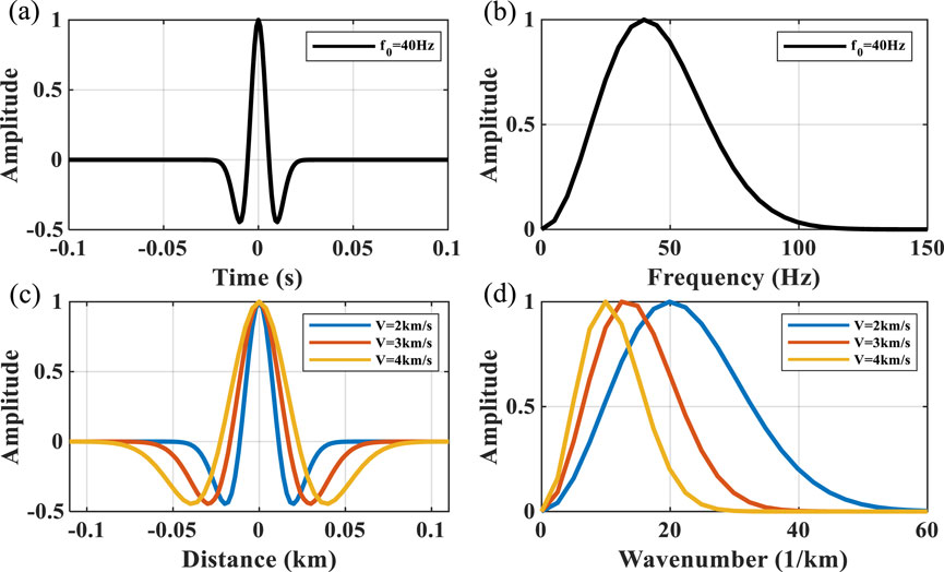
Figure 2. Single-wavelet comparison. (A) 40-Hz time-domain zero-phase Ricker wavelet. (B) Amplitude spectrum of the time-domain wavelet in the frequency domain. (C) Corresponding depth-domain wavelets for different velocities (2 km/s, 3 km/s, and 4 km/s). (D) Amplitude spectrum of depth-domain wavelets in the wavenumber domain.

Figure 3 shows the single-wavelet (i.e., sky-blue line shown in Figure 2C) depth–wavenumber spectrum experiments for different methods. It can be seen that WUST (Figure 3C) obtains a more accurate wavenumber spectrum than ST (Figure 3B) by removing the linear wavenumber-dependent term, but it performs poorly in the low-wavenumber region. By introducing parameters A and B, MWUST ensures that the wavenumber spectrum is accurate while performing well in the low-wavenumber region (Figures 3D–F). Figures 3D–F show that A plays a greater role in the depth–wavenumber spectrum than B, which is consistent with the conclusion reached in Figure 1. The amplitude spectra are extracted from the red dashed lines in Figure 3 to describe the wavenumber distribution in detail, as shown in Figure 4. Here, 1/3 and 10 are used for A and B in MWUST, respectively. It can be seen that the central frequency of the amplitude spectrum obtained based on the ST deviates from the reference frequency. However, MWUST matches the FT curve well, which further validates the advantages and effectiveness of the proposed method (i.e., MWUST) over ST and WUST.

Figure 3

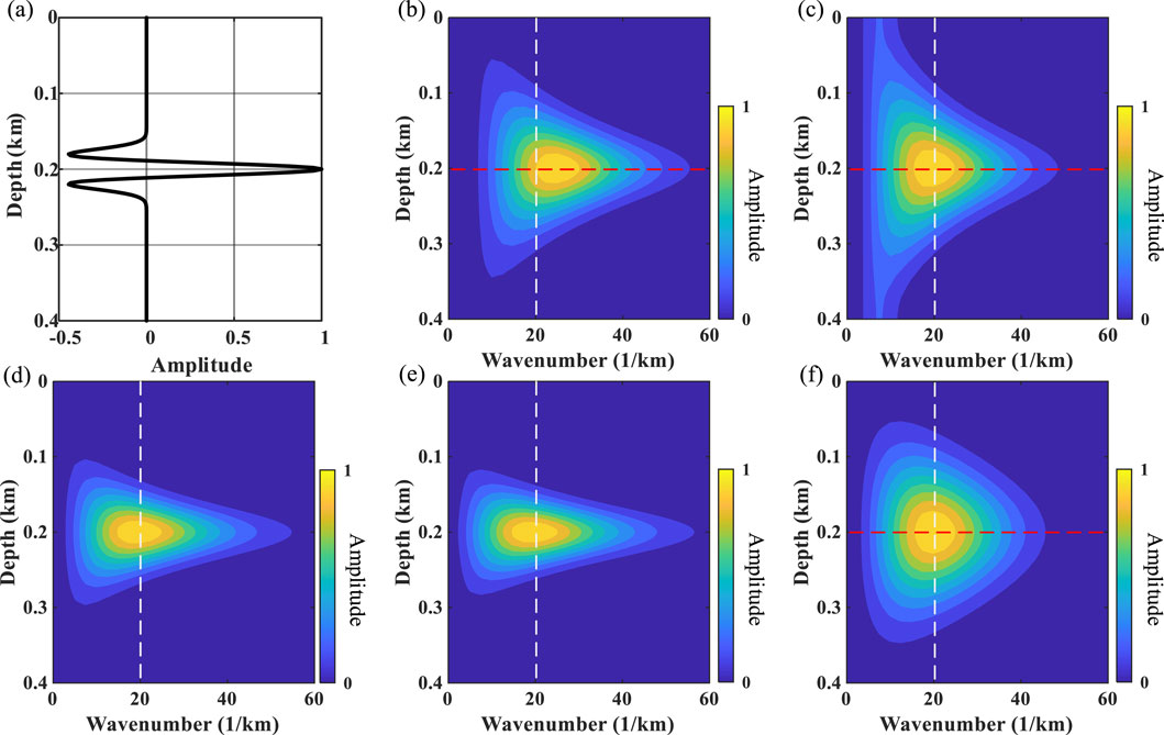
Figure 3. Depth–wavenumber spectrum of (A) the depth-domain wavelet with velocity 2 km/s obtained by (B) ST, (C) WUST, (D) MWUST (A = 4/3, B = 10), (E) MWUST (A = 4/3, B = 15), and (F) MWUST (A = 1/3, B = 10). The white dashed line indicates the reference wavenumber.

Figure 4

Figure 4. Amplitude spectrums of different methods (ST, WUST, and MWUST) at the locations shown by the red dashed lines in Figure 3.

Subsequently, a simple model in which the three reflection coefficients (Figure 5A) are related to the wavelet velocities mentioned in Figure 2C is used to perform wavelet estimation. Figures 6A–C show the depth–wavenumber spectrum of ST, WUST, and MWUST, where the black and red asterisks indicate the reference primary wavenumber of the signal at the position of the reflection coefficient and the primary wavenumber corresponding to the depth–wavenumber spectrum calculated by the different methods, respectively. It can be seen that the wavenumber distributions of WUST and MWUST match the reference values more closely than those of ST, but the depth–wavenumber spectrum of MWUST has a higher depth resolution in the low-wavenumber region (white arrows).

Figure 5

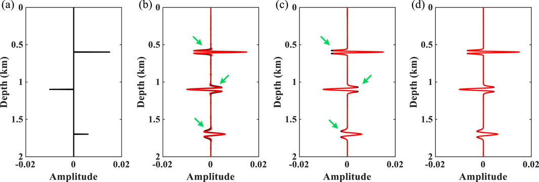
Figure 5. (A) Synthetic reflectivity series model. (B) Reference seismogram (black line) and reconstructed seismic records (red line) using the ST. (C) Reference seismogram (black line) and reconstructed seismic records (red line) using WUST. (D) Reference seismogram (black line) and reconstructed seismic records (red line) using MWUST.

Figure 6

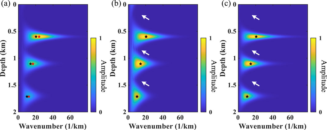
Figure 6. Depth–wavenumber spectrum of the three-wavelet model obtained using (A) ST, (B) WUST, and (C) MWUST (A = 4/3, B = 10).

Figures 7A–C show the depth-variant wavelets extracted from the depth–wavenumber spectrum obtained using different methods. Based on the known reflection coefficients, the depth-domain wavelets extracted by the different methods are convolved with them to obtain reconstructed seismic records, as shown by the red line in Figures 5B–D. The seismic records reconstructed by the proposed method (i.e., MWUST) are best matched to the reference seismogram (black line in Figure 5D). Figure 8 shows the normalized errors of the reconstructed seismic records of the wavelet extracted by the different methods. The white dashed line indicates the exact solution, i.e., the closer the focus is to the white dashed line, the more accurate the reconstructed result is. As expected, the more accurate depth–wavenumber spectrum obtained by MWUST resulted in more accurate extracted depth-domain wavelets, thus minimizing the error between the reconstructed seismogram and the reference seismogram.

Figure 7

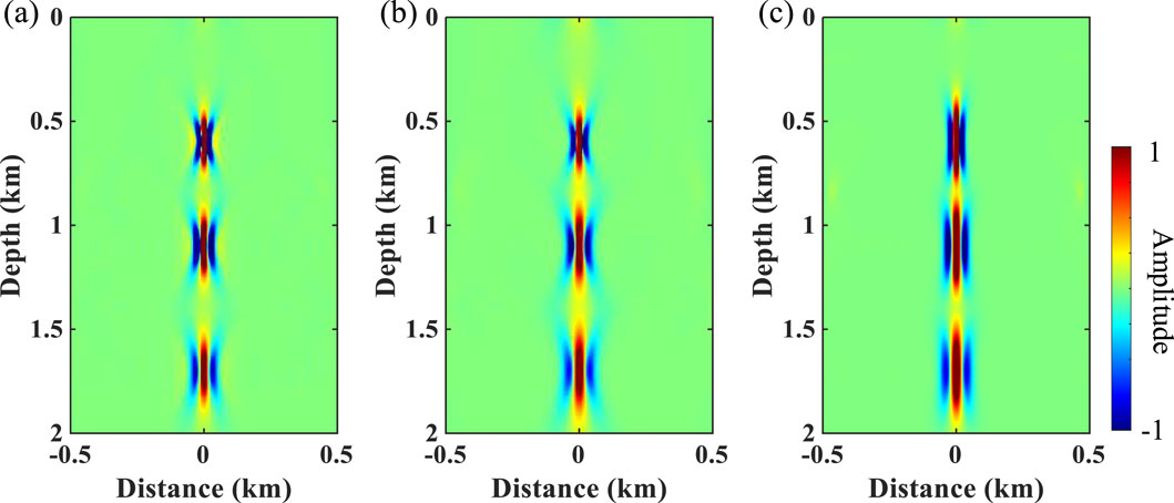
Figure 7. Depth-variant wavelets extracted from the depth–wavenumber spectrum obtained using (A) ST, (B) WUST, and (C) MWUST (A = 4/3, B = 10).

Figure 8

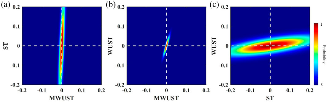
Figure 8. Normalized errors of the reconstructed seismic records of the wavelet extracted by the different methods.

3.2 Field data example

A more realistic example is further used to test the effectiveness of the method. The well–seismic ties between velocity curves and depth-domain seismic data (black lines) are displayed in Figure 9. Figures 10A–C show the depth–wavenumber spectrum of depth-domain seismic data using ST, WUST, and MWUST, respectively. The depth-variant wavelets extracted using the different methods are shown in Figures 11A–C. The reconstructed seismograms (red lines) obtained by combining known velocity well-log data and depth-domain wavelets extracted using the different methods are shown in Figures 9B–D. In this test, the density is assumed to be a constant density that does not vary with depth. The seismic records reconstructed (red lines) by the three methods roughly match the reference seismic records (black lines). However, the reconstructed seismic records of the proposed method are more consistent with the reference seismic records in some aspects compared to the reconstructed records of the other two methods (e.g., green arrows).

Figure 9

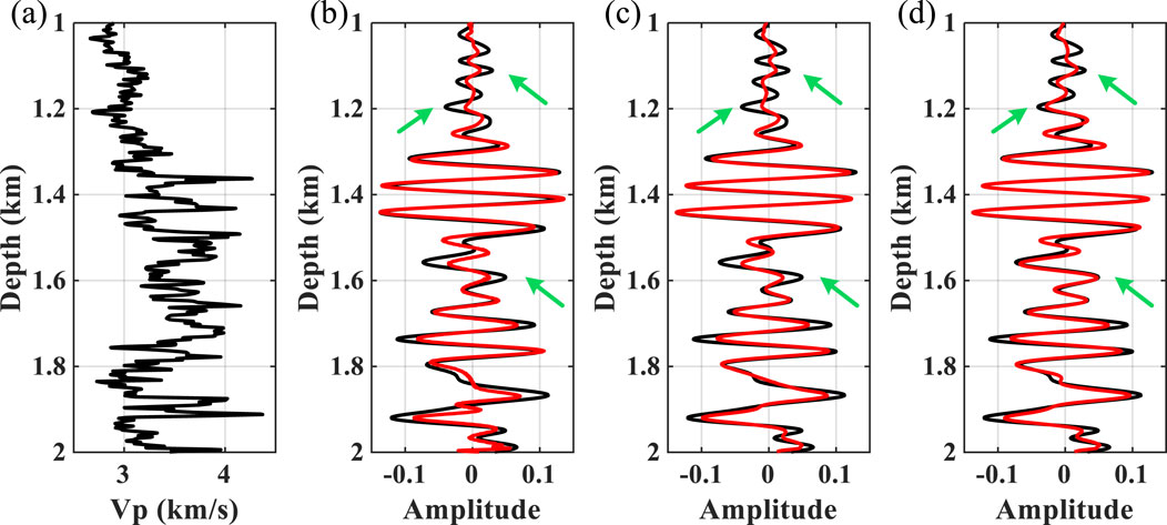
Figure 9. (A) Field well-log data of P-wave velocity. (B) Reference seismogram (black line) and reconstructed seismic records (red line) obtained using ST. (C) Reference seismogram (black line) and reconstructed seismic records (red line) obtained using WUST. (D) Reference seismogram (black line) and reconstructed seismic records (red line) obtained using MWUST (A = 4/3, B = 10).

Figure 10

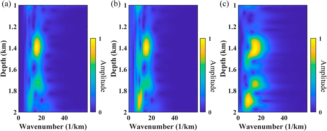
Figure 10. Depth–wavenumber spectrum of depth-domain seismic data obtained using (A) ST, (B) WUST, and (C) MWUST (A = 4/3, B = 10).

Figure 11

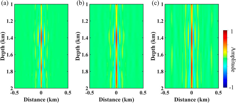
Figure 11. Depth-variant wavelets extracted from the depth–wavenumber spectrum obtained using (A) ST, (B) WUST, and (C) MWUST (A = 4/3, B = 10).

We perform further inversion tests to demonstrate the impact of the extracted wavelet on subsequent seismic inversion and interpretation. The algorithm used here is a Bayesian-based inversion method, the details of which can be found in Zhang et al. (2021a). In order to ensure a fair comparison of the inversion results, we perform the inversion by changing only the input wavelet, leaving the other inversion parameters unchanged. Figure 12 shows the inversion results obtained from the wavelet extracted by the different methods (i.e., ST, WUST, and MWUST) as input. It can be seen that the results obtained from the inversion of the wavelet extracted based on the ST show significant oscillations compared to those obtained from the inversion of the wavelets extracted by the other two methods. Although small differences are exhibited in the reconstructed seismic records (Figure 9B), the impact of the small errors on the inversion results is significant. The accuracy of the inversion results (green arrows in Figure 12) of the proposed method is greater due to the extraction of a more accurate depth-domain wavelet.

Figure 12

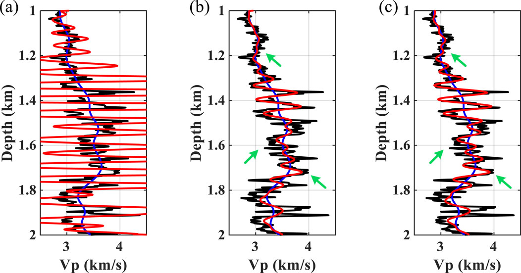
Figure 12. Inversion results obtained from the depth-domain wavelet extracted by the different methods as input. (A) ST, (B) WUST, and (C) MWUST (A = 4/3, B = 10). The black lines represent reference well-log curves, the red lines represent inversion results, and the blue lines represent the initial model.

4 Discussion

Many depth migration techniques have been developed to create depth-domain seismic datasets, which are increasingly being utilized for oil and gas exploration and demonstrate greater advantages over time-domain datasets. This places higher requirements on direct deep-domain processing and interpretation techniques, including depth-domain seismic inversion. To obtain reliable results from depth-domain seismic inversion, it is necessary to have an accurate depth-domain wavelet. The wavelet has two key parameters, dominant frequency and phase, mostly obtained from the depth–wavenumber spectrum for the depth-domain seismic data. To this end, we developed a workflow for extracting depth-variant wavelets to accommodate the potential non-stationarity of seismic data in the depth domain. The method improves the precision of wavenumber components by removing the linear term related to the wavenumber in the S-transform. Additionally, it introduces slope and intercept parameters to enhance the depth resolution at low wavenumbers, resulting in a more reliable depth–wavenumber spectrum. Then, on the premise that the reflectivity in the depth domain is a random sequence, the non-stationary wavelet can be accurately extracted based on the obtained depth–wavenumber spectrum. However, the proposed method is not limited to the extraction of non-stationary wavelets in the depth domain. Depending on the difference in the input spectrum, the proposed method can be easily extended to the extraction of seismic wavelets from both stationary and non-stationary signals in the time domain.

Zhang and Deng (2023) examined the impact of varying angles on seismic wavelets and extended the spectral decomposition-based wavelet extraction method to pre-stack seismic data. In this study, we focus on achieving a more precise spectrum by re-deriving the expression for the depth–wavenumber spectrum to ensure the accuracy of the subsequent wavelet extraction. This improved method is tested and validated using post-stack seismic data. Indeed, seismic gathers exhibit angle dependence in actual exploration processes, and it is crucial to consider the effects of this angle dependence. In addition, attenuation and dispersion effects of seismic signals during propagation through subsurface media are not considered. For future research, the proposed depth-domain wavelet estimation method is suggested to be improved by incorporating the depth-variant effects of seismic attenuation and dispersion. It is hoped to obtain a wavelet matrix that can more accurately characterize seismic wave propagation and improve the accuracy of subsequent reservoir prediction and interpretation.

5 Conclusion

An accurate depth-domain wavelet plays a crucial role in the reliable interpretation and inversion of depth-domain seismic data. In this paper, we propose a MWUST method to accomplish accurate depth-domain seismic wavelet estimation. The method obtains more accurate wavenumber distribution with guaranteed depth and wavenumber resolution, thus providing a prerequisite for reliable depth-domain wavelet estimation. Numerical experiments demonstrate the advantages of the proposed method over ST- and WUST-based wavelet extraction methods. We further apply depth-domain wavelets extracted using different methods to perform inversion tests and show that even small errors can lead to unreliable inversion results. This illustrates the importance of extracting an accurate wavelet for subsequent seismic inversion and interpretation, as well as the effectiveness of the proposed method. Additionally, the proposed method can be easily extended to the wavelet extraction of arbitrary non-stationary seismic data, in addition to its application to depth-domain seismic wavelet extraction.

Data availability statement

The raw data supporting the conclusion of this article will be made available by the authors, without undue reservation.

Author contributions

YX: conceptualization, methodology, writing–original draft, and writing–review and editing. JZ: software, supervision, and writing–review and editing. GZ: investigation, validation, and writing–review and editing. DZ: supervision and writing–review and editing.

Funding

The author(s) declare that financial support was received for the research, authorship, and/or publication of this article. This work was financially supported by the National Natural Science Foundation of China (42204108), the National Key Laboratory of Petroleum Resources and Engineering, China University of Petroleum, Beijing (PRE/open-2305), the Natural Science Foundation of Sichuan (2023NSFSC0768), and the Software Development Project for Concrete Defect Measurement and Processing at Multi-Layer Interfaces (2024-ZH004-N).

Conflict of interest

Authors GZ and DZ were employed by Sichuan Water Development Investigation, Design & Research Co., Ltd.

The remaining authors declare that the research was conducted in the absence of any commercial or financial relationships that could be construed as a potential conflict of interest.

Publisher’s note

All claims expressed in this article are solely those of the authors and do not necessarily represent those of their affiliated organizations, or those of the publisher, the editors, and the reviewers. Any product that may be evaluated in this article, or claim that may be made by its manufacturer, is not guaranteed or endorsed by the publisher.

References

Buland, A., and Omre, H. J. (2003). Bayesian wavelet estimation from seismic and well data. Geophysics 68 (6), 2000–2009. doi:10.1190/1.1635053

CrossRef Full Text | Google Scholar

Cai, R., Sun, C., Yao, Z. A., and Li, S. (2024). A depth-variant seismic wavelet extraction method for basis pursuit inversion with an impedance trend constraint. Geophysics 89 (3), R275–R286. doi:10.1190/geo2023-0255.1

CrossRef Full Text | Google Scholar

Danielsen, V., and Karlsson, T. (1984). Extraction of signatures from seismic and well data. First Break 2 (4), 15–21. doi:10.3997/1365-2397.1984008

CrossRef Full Text | Google Scholar

De Macedo, I. A., and De Figueiredo, J. J. S. J. (2020). On the seismic wavelet estimative and reflectivity recovering based on linear inversion: well-to-seismic tie on a real data set from Viking Graben, North Sea. Geophysics 85 (5), D157–D165. doi:10.1190/geo2019-0183.1

CrossRef Full Text | Google Scholar

George, N. V., Sahu, S. S., Mansinha, L., Tiampo, K., and Panda, G. (2009). Time localised band filtering using modified S-transform. IEEE 68, 42–46. doi:10.1109/icsps.2009.63

CrossRef Full Text | Google Scholar

Gunning, J., and Glinsky, M. E. (2006). Wavelet extractor: a Bayesian well-tie and wavelet extraction program. Comput. Geosci. 32 (5), 681–695. doi:10.1016/j.cageo.2005.10.001

CrossRef Full Text | Google Scholar

Ke, X., Shi, Y., Fu, X., Song, L., Jing, H., Yang, J., et al. (2023). The nth power Fourier spectrum analysis for the generalized seismic wavelets. IEEE Trans. Geoscience Remote Sens. 61, 1–10. doi:10.1109/tgrs.2023.3243184

CrossRef Full Text | Google Scholar

Laake, A., Zhang, R., and Deng, Z. (2019). Depth domain pre-stack seismic inversion with depth and angle variant wavelets. OnePetro, 1–5.

Google Scholar

Lazear, G. D. J. (1993). Mixed-phase wavelet estimation using fourth-order cumulants. Geophysics 58 (7), 1042–1051. doi:10.1190/1.1443480

CrossRef Full Text | Google Scholar

Li, D., Castagna, J., and Goloshubin, G. (2016). Investigation of generalized S-transform analysis windows for time-frequency analysis of seismic reflection data. Geophysics 81 (3), V235–V247. doi:10.1190/geo2015-0551.1

CrossRef Full Text | Google Scholar

Li, M., Lu, J., Stovas, A., and Wang, Y. (2022). Joint PP, PS1, and PS2 AVA inversion of HTI media. IEEE Trans. Geoscience Remote Sens. 60, 1–13. doi:10.1109/tgrs.2022.3170240

CrossRef Full Text | Google Scholar

Li, S., Peng, G., Wang, J., and Tian, T. (2020). Advantages and applications of seismic data interpretation in depth domain. OnePetro, 1–5.

Google Scholar

Lines, L. R., and Treitel, S. J. (1985). Wavelets, well logs and Wiener filters. First Break 3 (8), 9–14. doi:10.3997/1365-2397.1985014

CrossRef Full Text | Google Scholar

Paxton, A., Kholiq, A., Zhang, L., Shadlow, J., and Shadrina, M. (2022). Large-scale pre-stack seismic depth-domain inversion: a case study from the northern carnarvon basin. Offshore Australia: European Association of Geoscientists and Engineers, 1–5.

CrossRef Full Text | Google Scholar

Sacchi, M. D., and Ulrych, T. J. J. (2000). Nonminimum-phase wavelet estimation using higher order statistics. Lead. Edge 19 (1), 80–83. doi:10.1190/1.1438466

CrossRef Full Text | Google Scholar

Sengupta, M., Zhang, H., and Jervis, M. (2018). Direct depth domain elastic inversion. OnePetro, 206–510.

Google Scholar

Sengupta, M., Zhang, H., Zhao, Y., Jervis, M., and Grana, D. (2021). Direct depth-domain Bayesian amplitude-variation-with-offset inversion. 86(5): M167–M176. doi:10.1190/geo2020-0219.1

CrossRef Full Text | Google Scholar

Shadlow, J., Christiansen, D., Al-Houli, M., Paxton, A., and Wilson, T. (2022). Getting the most out of a large data set: a case study for a large 3D seismic interpretation project in the Carnarvon Basin, NW Australia. Lead. Edge 41 (12), 857–863. doi:10.1190/tle41120857.1

CrossRef Full Text | Google Scholar

Stockwell, R. G., Mansinha, L., and Lowe, R. (1996). Localization of the complex spectrum: the S transform. IEEE Trans. signal Process. 44 (4), 998–1001. doi:10.1109/78.492555

CrossRef Full Text | Google Scholar

Tang, Y., Chen, S., Wang, G., and Li, X. (2024). Depth-domain direct inversion based on the generalized unscaled S-transform method. Oslo, Norway: European Association of Geoscientists and Engineers, 1–5.

CrossRef Full Text | Google Scholar

Van Der Baan, M. (2008). Time-varying wavelet estimation and deconvolution by kurtosis maximization. Geophysics 73 (2), V11–V18. doi:10.1190/1.2831936

CrossRef Full Text | Google Scholar

Walden, A. T., and White, R. E. (1998). Seismic wavelet estimation: a frequency domain solution to a geophysical noisy input-output problem. IEEE Trans. Geoscience Remote Sens. 36 (1), 287–297. doi:10.1109/36.655337

CrossRef Full Text | Google Scholar

Wang, B. (2016). An amplitude preserving S-transform for seismic data attenuation compensation. IEEE Signal Process. Lett. 23 (9), 1155–1159. doi:10.1109/lsp.2016.2586445

CrossRef Full Text | Google Scholar

Wang, N., Shi, Y., Ni, J., Fang, J., and Yu, B. (2024). Enhanced seismic attenuation compensation: integrating attention mechanisms with residual learning in neural networks. IEEE Trans. Geoscience Remote Sens. 62, 1–11. doi:10.1109/tgrs.2024.3445130

CrossRef Full Text | Google Scholar

Wang, N., Xing, G., Zhu, T., Zhou, H., and Shi, Y. (2022a). Propagating seismic waves in VTI attenuating media using fractional viscoelastic wave equation. J. Geophys. Res. Solid Earth 127 (4), e2021JB023280. doi:10.1029/2021jb023280

CrossRef Full Text | Google Scholar

Wang, P., Cui, Y.-A., Chen, X., Pan, X., and Liu, J. (2022b). Analysis and application of the sparse prior in probabilistic prediction of elastic parameters. IEEE Trans. Geoscience Remote Sens. 60, 1–9. doi:10.1109/tgrs.2022.3181175

CrossRef Full Text | Google Scholar

Wu, L., and Castagna, J. (2017). S-transform and Fourier transform frequency spectra of broadband seismic signals. Geophysics 82 (5), O71–O81. doi:10.1190/geo2016-0679.1

CrossRef Full Text | Google Scholar

Yilmaz, Ö. (2001). Seismic data analysis: processing, inversion, and interpretation of seismic data. Tulsa: Society of exploration geophysicists.

Google Scholar

Zhang, J., Chen, X., Jiang, W., Liu, Y., and Xu, H. (2022a). Estimation of the depth-domain seismic wavelet based on velocity substitution and a generalized seismic wavelet model. Geophysics 87 (2), R213–R222. doi:10.1190/geo2020-0745.1

CrossRef Full Text | Google Scholar

Zhang, J., Li, J., Chen, X., and Li, Y. (2021a). Geological structure-guided hybrid MCMC and Bayesian linearized inversion methodology. J. Petroleum Sci. Eng. 199, 108296. doi:10.1016/j.petrol.2020.108296

CrossRef Full Text | Google Scholar

Zhang, J., Li, J., Chen, X., Li, Y., Huang, G., and Chen, Y. (2021b). Robust deep learning seismic inversion with a priori initial model constraint. Geophys. J. Int. 225 (3), 2001–2019. doi:10.1093/gji/ggab074

CrossRef Full Text | Google Scholar

Zhang, J., Li, J., Wang, S., Geng, W., and Cheng, W. (2022b). An improved unscale S transform in frequency domain. IEEE Geosci. Remote Sens. Lett. 20, 1–5. doi:10.1109/lgrs.2022.3232593

CrossRef Full Text | Google Scholar

Zhang, J., Zhao, X., Li, J., and Chen, X. (2022c). Structure-oriented prestack waveform inversion. Geophysics 87 (3), M73–M85. doi:10.1190/geo2021-0452.1

CrossRef Full Text | Google Scholar

Zhang, R., and Deng, Z. (2018). A depth variant seismic wavelet extraction method for inversion of poststack depth-domain seismic data. Geophysics 83 (6), R569–R579. doi:10.1190/geo2017-0816.1

CrossRef Full Text | Google Scholar

Zhang, R., and Deng, Z. (2023). Depth-domain angle and depth variant seismic wavelets extraction for prestack seismic inversion. Geophysics 88 (1), R1–R10. doi:10.1190/geo2021-0647.1

CrossRef Full Text | Google Scholar

Zhou, L., Liu, X., Li, J., and Liao, J. (2021). Robust AVO inversion for the fluid factor and shear modulus. Geophysics 86 (4), R471–R483. doi:10.1190/geo2020-0234.1

CrossRef Full Text | Google Scholar