 Lian Liu
 Bo Yang
 Yi Zhang
- School of Earth Sciences, Zhejiang University, Hangzhou, China
Artificial neural networks (ANN) have gained significant attention in magnetotelluric (MT) inversions due to their ability to generate rapid inversion results compared to traditional methods. While a well-trained ANN can deliver near-instantaneous results, offering substantial computational advantages, its practical application is often limited by difficulties in accurately fitting observed data. To address this limitation, we introduce a novel approach that customizes an auto-encoder (AE) whose decoder is replaced with the MT forward operator. This integration accounts for the governing physical laws of MT and compels the ANN to focus not only on learning the statistical relationships from data but also on producing physically consistent results. Moreover, because ANN-based inversions are sensitive to variations in observation systems, we employ scaling laws to transform real-world observation systems into formats compatible with the trained ANN. Synthetic and real-world examples show that our scheme can recover comparable results with higher computational efficiency compared to the classic Occam’s inversion. This study not only perfectly fits the observed data but also enhances the adaptability and efficiency of ANN-based inversions in complex real-world environments.
1 Introduction
Magnetotelluric (MT) inverse problems are inherently nonlinear and fail to produce a unique solution due to the limitations of observed data, the presence of noise, and the model’s inherent null space (Backus and Gilbert, 1967; Parker, 1983). Researchers typically employ deterministic methods (Tikhonov and Arsenin, 1977; Constable et al., 1987; Newman and Alumbaugh, 2000; Rodi and Mackie, 2001; Tarantola, 2004; Kelbert et al., 2014; Key, 2016) or stochastic approaches (Jackson and Matsu’ura, 1985; Grandis et al., 1999; Ray, 2021; Peng et al., 2022) to solve the inverse problems.
With the explosive development of deep learning, artificial neural network (ANN) (Roth and Tarantola, 1994; Langer et al., 1996) has shown considerable promise in MT inversion (Guo et al., 2020; Li R. et al., 2020; Guo et al., 2021; Liu W. et al., 2023; Liu et al., 2024 W.; Xu et al., 2024). ANN is a computational model inspired by the structure and function of the human brain. It consists of interconnected neurons that work together to process complex information (Bishop, 1995; Goodfellow et al., 2014; 2016). Such inversions have primarily relied on classic supervised learning (Liao et al., 2022; Xie et al., 2023; Liu X. et al., 2024), which is fundamentally underpinned by a mechanism akin to prior sampling-based strategies (Valentine and Sambridge, 2021). Generally, ANN learns a mapping from the feature space to the label space based on provided feature-label pairs. Then, we can apply this mapping to new features. Therefore, we need to construct a large number of geoelectric models serving as labels and estimate corresponding MT responses serving as features before training an ANN. The estimation of MT responses, typically generated through forward simulations, is straightforward. However, the construction of geoelectric models is challenging due to the complexity of Earth’s structures.
Considering the difficulty of model construction, there are two primary research directions. The first is integrating prior information from sources, such as logging, near-surface geology, and geostatistical data (Wang et al., 2023; Pan et al., 2024; Rahmani Jevinani et al., 2024). Alternatively, we can build geoelectric models using simple mathematical constraints, such as the assumption that the geoelectric model should be smooth (Ling et al., 2023; Liu L. et al., 2023), which is consistent with traditional linearized inversion results. The former is beneficial in improving the inversion resolution, and the latter is more generic for different structures of the Earth. Moreover, Pan et al. (2024) developed a neural network based on deformable convolution (Dai et al., 2017), which extracts hidden relationships and allows flexible adjustments in the size and shape of the feature region. Xu et al. (2024) utilized a self-attention mechanism (Levine et al., 2022) to enhance feature extraction. The supervised ANNs promote the development of MT inversions but have limitations in physical constraints and generalization: the MT response of the model recovered from the trained ANN may not fit the observed data, and we cannot reuse the trained ANN to invert new MT data, which are collected from a different observation system.
The auto-encoder (AE) can be considered a variant of supervised learning. It comprises two key components: an encoder that transforms input features into a user-specified parameter space and a decoder that reconstructs the input features from the specified space. The AE can be trained without labels by minimizing the difference between the reconstructed predictions and the original input features. To fit MT data better, researchers replaced the decoder with the MT forward operator to create a customized AE (Liu et al., 2020; 2022; Ling et al., 2024). In this configuration, the observed MT data serves as the input to the encoder, while the encoder’s output becomes the input to the MT forward operator, which generates the predicted data. Thus, the encoder’s output represents the geoelectric model. Since the MT forward operator is governed by established physical laws, the system is referred to as a physics-guided AE (PGAE). The framework is utilized not only in the MT method but also in other geophysical methods, such as seismic (Calderón-Macas et al., 1998; Liu B. et al., 2023), geosteering (Jin et al., 2019; Noh et al., 2022), and transient electromagnetic methods (Colombo et al., 2021; Wu et al., 2024).
MT data typically cover a frequency range spanning more than eight orders of magnitude (
In this study, we employ PGAE for the 1D inversion of MT data, which enables the inverted model to give better data fitting. At the same time, we incorporate scaling laws (Ward, 1967; Nabighian, 1987; Wong et al., 2009) to enhance the reusability of the trained ANN. Firstly, we introduce the fundamental theory for the MT method, PGAE, and scaling laws in Section 2. Subsequently, we demonstrate the efficacy of the proposed approach through applications to both synthetic and real-world MT data in Section 3. Finally, we provide a critical evaluation of the strengths and limitations of the proposed method.
2 Methodology
2.1 MT method
The MT method is a passive-source geophysical technique used to investigate the resistivity distribution of the Earth’s subsurface by analyzing the natural electromagnetic fields at the surface (Tikhonov, 1950; Cagniard, 1953). These fields mainly originate from regional and global thunderstorm activity, as well as the interaction of solar wind with the Earth’s magnetosphere. As electromagnetic waves propagate through the subsurface, their penetration depth is affected by the diffusion of waves, which varies with frequency. Specifically, waves with lower frequencies demonstrate a greater capacity for deeper penetration into geological structures. Since MT sources are sufficiently distant and the Earth possesses a higher refractive index than air, electromagnetic waves are assumed to propagate as planar waves perpendicular to the Earth’s surface. However, the diffusion process through various subsurface structures can exhibit arbitrary polarization. The MT method typically measures the orthogonal components of the natural electric and magnetic fields at the Earth’s surface, and a complex impedance tensor
where
The apparent resistivity and phase are defined as Equations 2, 3, respectively.
where
2.2 Physics-guided auto-encoder
Building on the AE framework, we replace the decoder with the MT forward operator to create a customized ANN (Figure 1). The loss function
where

Figure 1. The proposed PGAE framework.
Algorithm 1 outlines the workflow for implementing PGAE. The process begins by initializing the encoder parameters using a truncated normal distribution, which helps mitigate the exploding or vanishing gradient problems during training Li H. et al. (2020). After initialization, the training samples are shuffled randomly, and a batch of samples is selected and fed into the encoder to generate the corresponding geoelectric models. The MT forward operator is then applied to produce the predicted MT data. Subsequently, the loss function is evaluated using Equation 4. These steps constitute the forward propagation phase. Next, the gradient
Algorithm 1.The PGAE training algorithm.
Input: Initialize ANN weights
1 while
2 Shuffle the samples randomly and divide into
3 foreach batch do
4 Compute
5 Compute
6 Compute the gradient
7 Update
8 if
9 save
2.3 Scaling laws
Scaling laws provide a crucial theoretical framework for simulating the electromagnetic response of real-world resistivity structures within a laboratory setting (Ward, 1967; Nabighian, 1987; Wong et al., 2009). Building on the foundational work of Ward (1967), we utilize the coordinates
Ignoring the displacement current, the MT field is described by the diffusive forms of Maxwell’s equations with a time-dependent component
where
For the model-scale system, we have
Generally, we want the fields from the real-world system to be linearly transformed from the model-scale system, that is
where
Putting Equations 9–16 together, we have
According to Equations 17, 18, to simulate the MT response of real-world resistivity structures in a model-scale system, we should ensure that the model-scale system has the same induction number as the real-world system:
where
Scaling laws enable us to model large-scale MT responses using a small-size model. While researchers generally employ these principles for physical modeling, they are also applicable to numerical modeling. When we have an ANN trained for audio-frequency MT tasks, we can leverage the trained network to invert long-period MT data by applying scaling laws, rather than training a new network from scratch. Additionally, discrepancies between the number of frequencies in the real-world data and those used in training present another challenge. A practical solution is to interpolate the frequency sampling of the real-world data to match that of the training set. The interpolation method will perform effectively since MT apparent resistivity curves are typically smooth.
3 Numerical experiments
Recent research has established the effectiveness of employing ANNs to address the 1D MT inverse problem with a fixed observation system. Nonetheless, the application of ANNs to 2D and 3D problems remains largely exploratory. Therefore, we demonstrate the integration of PGAE and scaling laws in the 1D inversion of both synthetic and real-world MT data, highlighting their potential for enhancing inversion accuracy and generalization capabilities.
3.1 Obtaining a well-trained ANN
To prepare the training dataset, we analytically compute the apparent resistivity curves for 1D layered Earth models consisting of 31 layers and 25 frequencies, ranging from 10,000 Hz–1 Hz. The thicknesses of the layers begin at 20 m and increase logarithmically, as described in Equation 20, with the final layer always being a homogeneous half-space. For the resistivity of each layer, we uniformly sample values within the range of 0.1–100,000
where
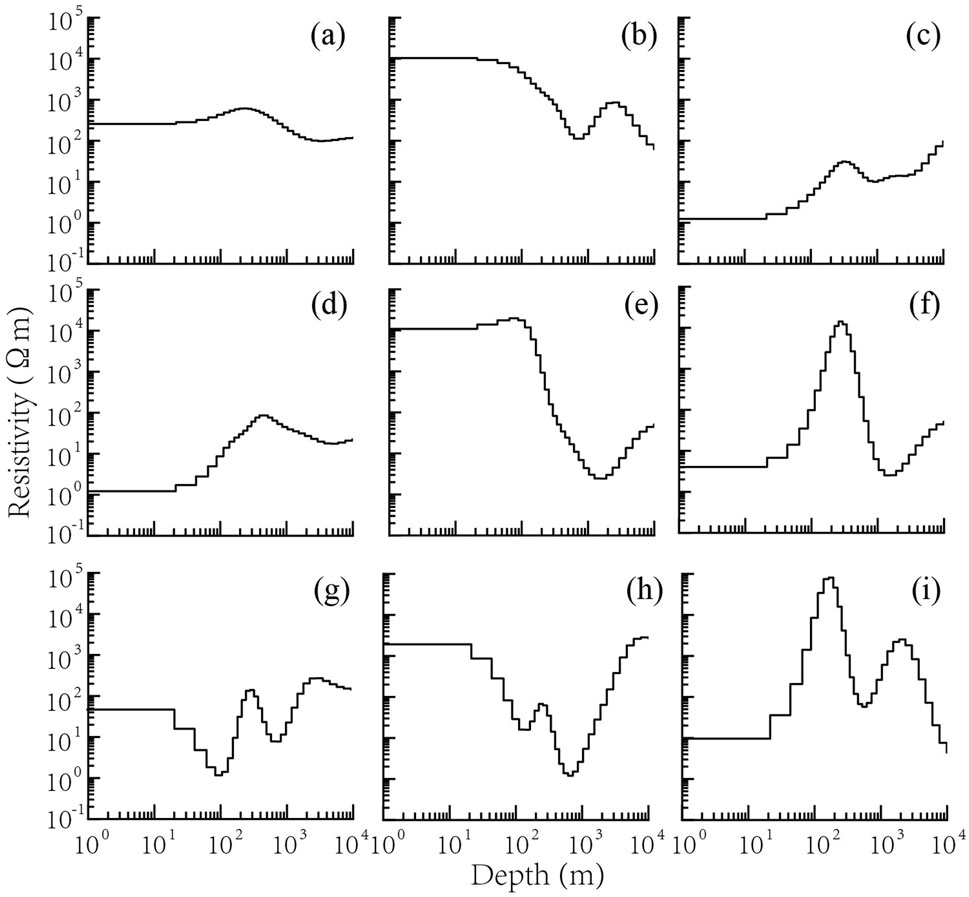
Figure 2. Random smooth models (A–I) generated according to Liu L. et al. (2023).
The primary objective of this study is to enhance the generalization capabilities of the trained ANN rather than to design a high-performance ANN. Accordingly, we employ an ANN architecture that is as simple as possible. Specifically, we construct an ANN with a single hidden layer containing 500 neurons. The number of neurons in the input (output) layer corresponds to the MT data (geoelectric model) used in the training dataset. The regularization parameter
We use the Adam optimizer to train the established network, as illustrated in Figure 3A, the data misfit decreases rapidly as the number of training epochs increases. A significant reduction in data misfit is observed at the end of the first epoch, indicating that the training of the network converges quickly. The gradual increase in model roughness shown in Figure 3B suggests that the well-trained PGAE possesses the capability to produce models with complex structures. After 20 epochs, the loss function, data misfit, and model roughness exhibit minimal changes, indicating the completion of the training stage. The network was trained using an NVIDIA Tesla K80 GPU with 12 GB of onboard memory, taking approximately 40 min.
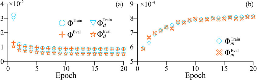
Figure 3. The loss function variations during training and evaluating. (A) the total loss function in training (sky-blue circles) and evaluating (orange crosses) and the data misfit in training (sky-blue triangles) and evaluating (orange stars). (B) the model roughness in training (sky-blue diamonds) and evaluating (orange crosses).
3.2 Synthetic examples
To evaluate the performance of the trained PGAE, we simulate numerous synthetic 1D MT data as test samples, which share the same observation frequencies as the training samples. For comparative analysis, we also invert these synthetic data using the classical Occam’s inversion (Constable et al., 1987). To further assess the noise adaptability of the trained PGAE, we introduce 5% Gaussian noise into the test samples. As illustrated in Figures 4, 5, the well-trained PGAE produces models comparable to those generated by the Occam’s inversion, with both methods yielding a satisfactory data fit.
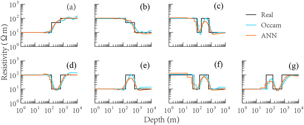
Figure 4. Inversion results of different synthetic data (A–G). The real (black) and inverted models, obtained from PGAE (orange) and Occam’s inversion (sky-blue), are shown as solid lines.
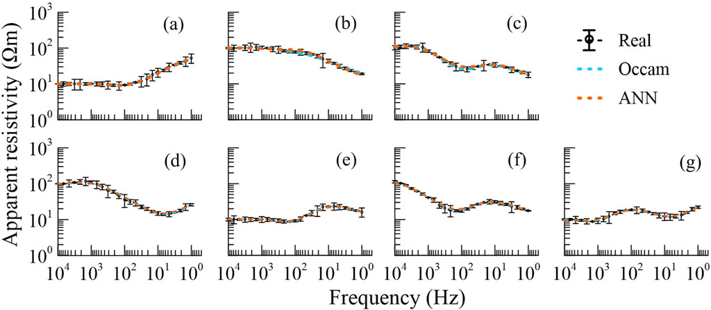
Figure 5. Fitting results of different synthetic data (A–G). The apparent resistivity curves are shown as dashed lines in corresponding colors as Figure 4. Error bars are plotted on the observed curves.
Although no noise was intentionally added to the training samples, the network demonstrates remarkable adaptability to noise. Given that noise is unavoidable in real-world data, we further evaluate the noise tolerance of the trained PGAE by testing it against three higher levels of Gaussian noise: 10%, 20%, and 30%. As illustrated in Figures 6, 7, the models predicted by the PGAE are comparable to those derived from the Occam’s inversion, indicating that the PGAE exhibits significant noise tolerance even at high levels of Gaussian noise.

Figure 6. Inversion results of the noisier data. (A–C) have the same real model, and (D–F) have the same real model. Percentages denote the noise levels. The lines and colors are the same as in Figure 4.
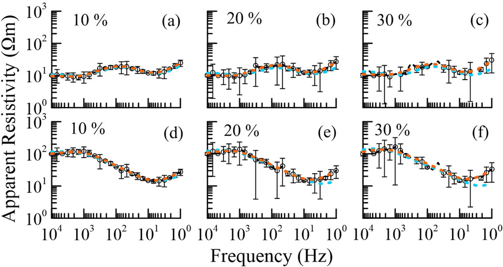
Figure 7. Fitting results of the noisier data. (A–C) have the same real model, and (D–F) have the same real model. Percentages denote the noise levels. The lines and colors are the same as in Figure 5.
3.3 Real-world examples
We select 11 MT sites recorded in the Tarim Basin for our real-world examples (Figure 8). The phase tensor analysis (Caldwell et al., 2004) shows that the resistivity distribution in the shallow area closely resembles a 1D structure (Figure 9), suitable for 1D inversion. Data from these sites were recorded using the Phoenix MTU-V5 system over approximately 22 h during the summer of 2019 and subsequently processed with the robust MT time series processing code, EMTF (Egbert and Booker, 1986), to estimate the impedance and vertical transfer functions. We utilize 41 frequencies ranging from 515 Hz to 0.0439 Hz, which share a similar bandwidth with the frequencies of the training samples but employ distinct frequency values. This enables the application of the scaling laws described in Section 2.3.
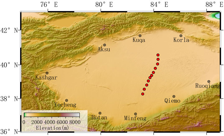
Figure 8. The study area of the real-world data in Tarim Basin. Red-filled circles represent the MT sites.
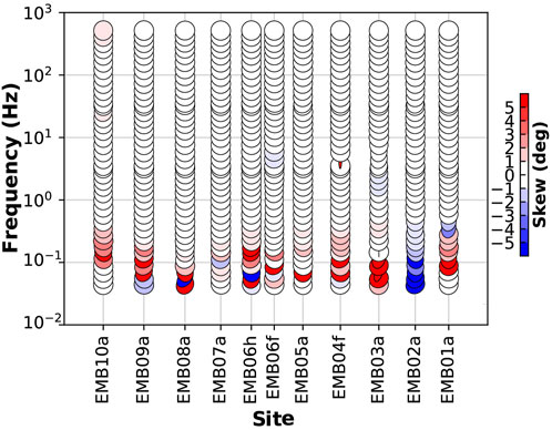
Figure 9. Phase tensors for all the frequencies from the survey line in Figure 8. Plotted using the MTpy library (Krieger and Peacock, 2014).
As illustrated in Figure 10, we first transform the frequencies of the real-world data to align with the frequency range of the training data. Subsequently, we employ the linear interpolation algorithm to match the number of real-world data to the neurons of the input layer of the trained ANN. Once the trained ANN generates an inverted model, the final step is transforming it back to its original scale, ensuring consistency with the real-world system. In this scenario, we scale the real-world frequencies by 10000/515, resistivity by 10, and model size by
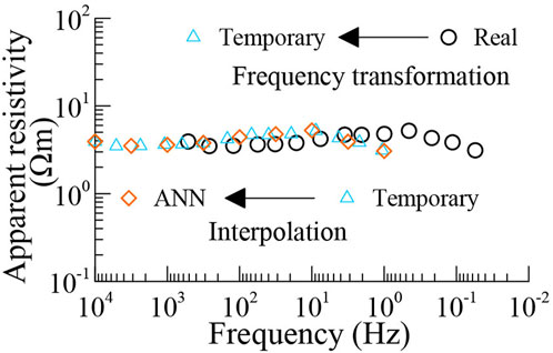
Figure 10. Predicting process of the well-trained ANN with scaling laws.
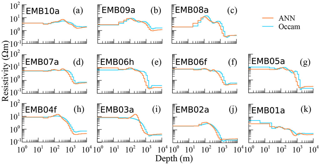
Figure 11. Inversion results of the real-world data. (A–K) indicate the sequence of MT sites along the survey line (SW-NE). The lines and colors are the same as in Figure 4.
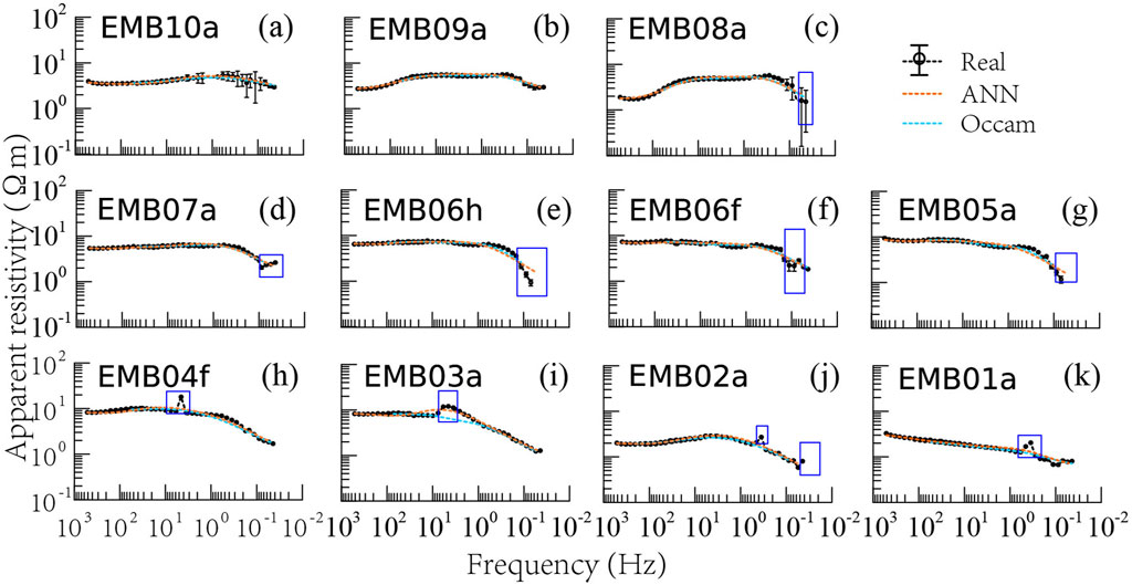
Figure 12. Fitting results of the real-world data. (A–K) indicate the sequence of MT sites along the survey line (SW-NE). Blue boxes mark the deleted outliers for 1D Occam’s inversion. The lines and colors are the same as in Figure 5.
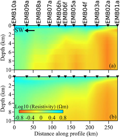
Figure 13. The electrical resistivity pseudo-sections of the real-world example produced by (A) PGAE and (B) Occam’s inversion.
4 Discussion and conclusion
The numerical experiments demonstrate that PGAE enhanced by scaling laws performs well, producing comparable models as the class Occam’s inversion does with higher efficiency after being well-trained. Here, we discuss its advantages and flaws in three aspects: model complexity, network architecture, and reusability of the network.
Model complexity is a formidable barrier for ANN-based MT inversions, limiting both the accuracy and generalization of these methods across diverse geological settings. The real-world resistivity models are inherently complex due to the highly heterogeneous nature of the Earth’s crust and mantle (Chave and Jones, 2012). This complexity is further compounded by varying geological features, such as fault zones, fluid-bearing formations, and volcanic structures. In traditional inversion methods (Kelbert et al., 2014; Key, 2016), model complexity can be managed through regularization techniques and by setting constraints based on prior geological information. The supervised ANNs (Liao et al., 2022; Xie et al., 2023; Liu X. et al., 2024), while powerful, are inherently data-driven and lack a physical basis. Addressing the challenge requires advances in hybrid modeling techniques and the integration of prior knowledge into the ANN framework to balance data-driven learning with geological realism. PGAE employs the forward operator as a decoder, which includes the physical laws behind the specific inverse problem. The framework can train networks without labels (models) and give a chance to add prior constraints into the training stage, which will significantly enhance the ability to reveal complex models. Moreover, future training datasets should include both synthetic and real-world data, which provide more real information related to the real tectonic and geological background.
Regarding the network architecture, it is not the primary focus of our study in the current stage. We focused on exploring the fundamental idea of PGAE, hence employing a straightforward and simple enough network with only one hidden layer. This simple design demonstrates a satisfactory ability to map the data space to the model space for 1D MT problems. However, the architecture may become crucial when addressing higher-dimensional inverse problems due to the significantly increased number of unknowns (Xu et al., 2024). A network with an insufficient degree of freedom, meaning an inadequate number of network parameters, may struggle to train effectively on the provided samples. Consequently, it would likely exhibit poor prediction performance when applied to real-world data. Conversely, while a network endowed with an excessive degree of freedom can be easily trained to fit the training and evaluation samples, this requires considerable computational time. Additionally, it may lead to overfitting, which poses challenges in maintaining the network’s generalization capabilities (Bishop, 1995). This problem is particularly pronounced in MT inversions, where the resistivity structure changes significantly with depth and electromagnetic responses are frequency-dependent. Each frequency corresponds to different depths, necessitating the ANN to learn the relationships across a broad spectrum of frequencies accurately. Theoretically, no established mathematical principles definitively determine the optimal network architecture (LeCun et al., 2015; Goodfellow et al., 2016), making trial-and-error the only practical approach to designing a network.
In previous studies (e.g., Ling et al., 2023; Pan et al., 2024), trained networks cannot be reused and must be re-trained from scratch when the observation system changes. However, our study makes an important step towards improving the reusability of well-trained ANNs in different observation systems. For 1D MT inverse problems, only variations in frequency range should be considered. By applying scaling laws, the trained ANN can be used in cases with nearly identical frequency bandwidths, expanding its applicability. When the frequency range of a new application spans different orders of magnitude, the trained ANN may lose its effectiveness. Therefore, it is essential to train separate ANNs tailored to different bandwidths to ensure reliable performance across a broader range of scenarios. For 3D problems, the complexity of the observation system increases further. Differences in site locations must be considered to ensure the reusability of trained ANNs. As site locations significantly affect the data characteristics in MT inversions, data from a new group of sites cannot be directly applied to the trained network without some transformation. Thus, data reconstruction between different site groups is a critical factor that must be addressed in future ANN-based MT inversion efforts. Techniques such as compressed sensing (Donoho, 2006), which can transform data from one set of locations to another, may offer potential solutions to this issue. Developing robust methods for data reconstruction should be a significant challenge.
In summary, we utilized PGAE along with scaling laws to improve the accuracy and generalization of the well-trained ANN for MT inversion. Specifically, PGAE takes into account the data misfit, while scaling laws enable the ANN to perform effectively even when the frequency range of an MT survey differs from the range used during the network’s original training. Fully enhancing the practicability, efficiency, and dependability of ANN-based inversions, particularly in the context of complex MT inverse problems, will require further research and innovation. Future research should focus on improving the adaptability of trained ANNs to both model complexity and observation systems, thereby increasing the utility of ANNs across diverse MT applications. Overcoming these challenges will be critical before ANN-based methods can be widely adopted in industry-level MT inversion software.
Data availability statement
The datasets presented in this study can be found in online repositories. The names of the repository/repositories and accession number(s) can be found below: https://github.com/Geo-LianLiu/MTPGAE.
Author contributions
LL: Conceptualization, Formal Analysis, Investigation, Methodology, Software, Validation, Writing–original draft. BY: Funding acquisition, Resources, Supervision, Validation, Writing–review and editing. YZ: Conceptualization, Investigation, Methodology, Validation, Writing–review and editing.
Funding
The author(s) declare that financial support was received for the research, authorship, and/or publication of this article. This research was financially supported by NSFC (grant 42474103).
Acknowledgments
We thank the editors and reviewers for their helpful suggestions.
Conflict of interest
The authors declare that the research was conducted in the absence of any commercial or financial relationships that could be construed as a potential conflict of interest.
Generative AI statement
The author(s) declare that no Generative AI was used in the creation of this manuscript.
Publisher’s note
All claims expressed in this article are solely those of the authors and do not necessarily represent those of their affiliated organizations, or those of the publisher, the editors and the reviewers. Any product that may be evaluated in this article, or claim that may be made by its manufacturer, is not guaranteed or endorsed by the publisher.
References
Backus, G. E., and Gilbert, J. F. (1967). Numerical applications of a formalism for geophysical inverse problems. Geophys. J. Int. 13, 247–276. doi:10.1111/j.1365-246X.1967.tb02159.x
Berdichevsky, M. N. (1976). “Basic principles of interpretation of magnetotelluric sounding curves,” in Geoelectric and geothermal studies (East-Central europe, soviet asia), KAPG geophysical monograph, 165–221Publisher. Budapest: Akademiai Kiado.
Cagniard, L. (1953). Basic theory of the magneto-telluric method of geophysical prospecting. Geophysics 18, 605–635. doi:10.1190/1.1437915
Calderón-Macas, C., Sen, M. K., and Stoffa, P. L. (1998). Automatic NMO correction and velocity estimation by a feedforward neural network. Geophysics 63, 1696–1707. doi:10.1190/1.1444465
Caldwell, T. G., Bibby, H. M., and Brown, C. (2004). The magnetotelluric phase tensor. Geophys. J. Int. 158, 457–469. doi:10.1111/j.1365-246x.2004.02281.x02281.x
Chave, A. D., and Jones, A. G. (2012). The magnetotelluric method: theory and practice. Cambridge University Press.
Colombo, D., Turkoglu, E., Li, W., Sandoval-Curiel, E., and Rovetta, D. (2021). Physics-driven deep-learning inversion with application to transient electromagnetics. Geophysics 86, E209–E224. doi:10.1190/geo2020-0760.1
Constable, S. C., Parker, R. L., and Constable, C. G. (1987). Occam’s inversion: a practical algorithm for generating smooth models from electromagnetic sounding data. Geophysics 52, 289–300. doi:10.1190/1.1442303
Dai, J., Qi, H., Xiong, Y., Li, Y., Zhang, G., Hu, H., et al. (2017). “Deformable convolutional networks,” in 2017 IEEE international conference on computer vision (ICCV), 764–773. doi:10.1109/ICCV.2017.89
Donoho, D. L. (2006). Compressed sensing. IEEE Trans. Inf. theory 52, 1289–1306. doi:10.1109/tit.2006.871582
Egbert, G. D., and Booker, J. R. (1986). Robust estimation of geomagnetic transfer functions. Geophys. J. R. Astronomical Soc. 87, 173–194. doi:10.1111/j.1365-246X.1986.tb04552.x
Goodfellow, I. J., Pouget-Abadie, J., Mirza, M., Xu, B., Warde-Farley, D., Ozair, S., et al. (2014). Generative adversarial networks. arXiv:1406.2661 [cs, stat]
Grandis, H., Menvielle, M., and Roussignol, M. (1999). Bayesian inversion with Markov chains-I. The magnetotelluric one-dimensional case. Geophys. J. Int. 138, 757–768. doi:10.1046/j.1365-246x.1999.00904.x
Guo, R., Li, M., Yang, F., Xu, S., and Abubakar, A. (2020). Application of supervised descent method for 2D magnetotelluric data inversion. Geophysics 85, WA53–WA65. doi:10.1190/geo2019-0409.1
Guo, R., Yao, H. M., Li, M., Ng, M. K. P., Jiang, L., and Abubakar, A. (2021). Joint inversion of audio-magnetotelluric and seismic travel time data with deep learning constraint. IEEE Trans. Geoscience Remote Sens. 59, 7982–7995. doi:10.1109/TGRS.2020.3032743
Jackson, D. D., and Matsu’ura, M. (1985). A Bayesian approach to nonlinear inversion. J. Geophys. Res. Solid Earth 90, 581–591. doi:10.1029/JB090iB01p00581
Jin, Y., Wu, X., Chen, J., and Huang, Y. (2019). “Using a physics-driven deep neural network to solve inverse problems for lwd azimuthal resistivity measurements,” in SPWLA annual logging symposium (SPWLA).D053S015R002
Kelbert, A., Meqbel, N., Egbert, G. D., and Tandon, K. (2014). ModEM: a modular system for inversion of electromagnetic geophysical data. Comput. and Geosciences 66, 40–53. doi:10.1016/j.cageo.2014.01.010
Key, K. (2016). MARE2DEM: a 2-D inversion code for controlled-source electromagnetic and magnetotelluric data. Geophys. J. Int. 207, 571–588. doi:10.1093/gji/ggw290
Kingma, D. P., and Ba, J. (2017). Adam: a method for stochastic optimization. arXiv:1412.6980 [cs] ArXiv: 1412.6980
Krieger, L., and Peacock, J. R. (2014). MTpy: a Python toolbox for magnetotellurics. Comput. and Geosciences 72, 167–175. doi:10.1016/j.cageo.2014.07.013
Langer, H., Nunnari, G., and Occhipinti, L. (1996). Estimation of seismic waveform governing parameters with neural networks. J. Geophys. Res. Solid Earth 101, 20109–20118. doi:10.1029/96JB00948
LeCun, Y., Bengio, Y., and Hinton, G. (2015). Deep learning. Nature 521, 436–444. doi:10.1038/nature14539
Levine, Y., Wies, N., Sharir, O., Cohen, N., and Shashua, A. (2022). “Tensors for deep learning theory,” in Tensors for data processing (Elsevier), 215–248. doi:10.1016/B978-0-12-824447-0.00013-3
Li, H., Krek, M., and Perin, G. (2020a). “A comparison of weight initializers in deep learning-based side-channel analysis,”. Applied cryptography and network security workshops. Editor J. e. a. Zhou (Cham: Springer International Publishing), 12418, 126–143. doi:10.1007/978-3-030-61638-0
Li, R., Yu, N., Wang, X., Liu, Y., Cai, Z., and Wang, E. (2020b). Model-based synthetic geoelectric sampling for magnetotelluric inversion with deep neural networks. IEEE Trans. Geoscience Remote Sens. 60, 1–14doi. doi:10.1109/TGRS.2020.3043661
Liao, X., Shi, Z., Zhang, Z., Yan, Q., and Liu, P. (2022). 2D inversion of magnetotelluric data using deep learning technology. Acta Geophys. 70, 1047–1060. doi:10.1007/s11600-022-00773-z
Ling, W., Pan, K., Ren, Z., Xiao, W., He, D., Hu, S., et al. (2023). One-dimensional magnetotelluric parallel inversion using a ResNet1D-8 residual neural network. Comput. and Geosciences 180, 105454. doi:10.1016/j.cageo.2023.105454
Ling, W., Pan, K., Zhang, J., He, D., Zhong, X., Ren, Z., et al. (2024). A 3-D magnetotelluric inversion method based on the joint data-driven and physics-driven deep learning technology. IEEE Trans. Geoscience Remote Sens. 62, 1–13. doi:10.1109/TGRS.2024.3369179
Liu, B., Jiang, P., Wang, Q., Ren, Y., Yang, S., and Cohn, A. G. (2023a). Physics-driven self-supervised learning system for seismic velocity inversion. Geophysics 88, R145–R161. doi:10.1190/geo2021-0302.1
Liu, L., Yang, B., and Xu, Y. (2020). “Solving geophysical inverse problems based on physics-guided artificial neural network,” in 2020 annual Meeting of Chinese geoscience union abstracts (chongqing), 314–316. doi:10.26914/c.cnkihy.2020.059737
Liu, L., Yang, B., Xu, Y., and Yang, D. (2023b). “Magnetotelluric inversion using supervised learning trained with random smooth geoelectric models,” in Third international meeting for applied geoscience and energy expanded abstracts, 489–492. doi:10.1190/image2023-3910431.1
Liu, L., Yang, B., Zhang, Y., Xu, Y., Peng, Z., and Yang, D. (2024a). Calculating sensitivity or gradient for geophysical inverse problems using automatic and implicit differentiation. Comput. and Geosciences 193, 105736. doi:10.1016/j.cageo.2024.105736
Liu, W., Wang, H., Xi, Z., Wang, L., Chen, C., Guo, T., et al. (2024b). Multitask learning-driven physics-guided deep learning magnetotelluric inversion. IEEE Trans. Geoscience Remote Sens. 62, 1–16. doi:10.1109/TGRS.2024.3457893
Liu, W., Wang, H., Xi, Z., and Zhang, R. (2023c). Smooth deep learning magnetotelluric inversion based on physics-informed Swin Transformer and multiwindow Savitzky–Golay filter. IEEE Trans. Geoscience Remote Sens. 61, 1–14. doi:10.1109/TGRS.2023.3304313
Liu, W., Wang, H., Xi, Z., Zhang, R., and Huang, X. (2022). Physics-driven deep learning inversion with application to magnetotelluric. Remote Sens. 14, 3218. doi:10.3390/rs14133218
Liu, X., Craven, J. A., Tschirhart, V., and Grasby, S. E. (2024c). Estimating three-dimensional resistivity distribution with magnetotelluric data and a deep learning algorithm. Remote Sens. 16, 3400. doi:10.3390/rs16183400
Meng, J., Wang, S., Cheng, W., Wang, Z., and Yang, L. (2022). Avo inversion based on transfer learning and low-frequency model. IEEE Geoscience Remote Sens. Lett. 19, 1–5. doi:10.1109/LGRS.2021.3132426
Nabighian, M. N. (1987). Electromagnetic methods in applied geophysics: volume 1, theory. Houston, Texas: Society of Exploration Geophysicists. doi:10.1190/1.9781560802631
Newman, G. A., and Alumbaugh, D. L. (2000). Three-dimensional magnetotelluric inversion using non-linear conjugate gradients. Geophys. J. Int. 140, 410–424. doi:10.1046/j.1365-246x.2000.00007.x
Noh, K., Pardo, D., and Torres-Verdín, C. (2022). 2.5-d deep learning inversion of lwd and deep-sensing em measurements across formations with dipping faults. IEEE Geoscience Remote Sens. Lett. 19, 1–5. doi:10.1109/LGRS.2021.3128965
Pan, K., Ling, W., Zhang, J., Zhong, X., Ren, Z., Hu, S., et al. (2024). MT2DInv-Unet: a 2D magnetotelluric inversion method based on deep-learning technology. Geophysics 89, G13–G27. doi:10.1190/geo2023-0004.1
Parker, R. L. (1983). The magnetotelluric inverse problem. Geophys. Surv. 6, 5–25. doi:10.1007/BF01453993
Peng, R., Han, B., Liu, Y., and Hu, X. (2022). A Julia software package for transdimensional Bayesian inversion of electromagnetic data over horizontally stratified media. Geophysics 87, F55–F66. doi:10.1190/geo2021-0534.1
Rahmani Jevinani, M., Habibian Dehkordi, B., Ferguson, I. J., and Rohban, M. H. (2024). Deep learning-based 1-D magnetotelluric inversion: performance comparison of architectures. Earth Sci. Inf. 17, 1663–1677. doi:10.1007/s12145-024-01233-6
Ray, A. (2021). Bayesian inversion using nested trans-dimensional Gaussian processes. Geophys. J. Int. 226, 302–326. doi:10.1093/gji/ggab114
Rodi, W., and Mackie, R. L. (2001). Nonlinear conjugate gradients algorithm for 2-D magnetotelluric inversion. Geophysics 66, 174–187. doi:10.1190/1.1444893
Roth, G., and Tarantola, A. (1994). Neural networks and inversion of seismic data. J. Geophys. Res. 99, 6753–6768. doi:10.1029/93JB01563
Tarantola, A. (2004). Inverse problem theory and methods for model parameter estimation. USA: Society for Industrial and Applied Mathematics.
Tikhonov, A. (1950). On determining electrical characteristics of the deep layers of the Earth’s crust, 73. Leningrad: Dokl. Akad. Nauk. SSSR, 295–297.
Tikhonov, A. N., and Arsenin, V. Y. (1977). Solutions of ill-posed problems. Hoboken, New Jersey: John Wiley & Sons.
Valentine, A., and Sambridge, M. (2021). Emerging directions in geophysical inversion. Phys. ArXiv 2110.06017. doi:10.48550/arXiv.2110.06017
Wang, H., Liu, Y., Yin, C., Su, Y., Zhang, B., and Ren, X. (2023). Flexible and accurate prior model construction based on deep learning for 2-D magnetotelluric data inversion. IEEE Trans. Geoscience Remote Sens. 61, 1–11. doi:10.1109/TGRS.2023.3239105
Wang, X., Jiang, P., Deng, F., Wang, S., Yang, R., and Yuan, C. (2024). Three-dimensional magnetotelluric forward modeling through deep learning. IEEE Trans. Geoscience Remote Sens. 62, 1–13. doi:10.1109/TGRS.2024.3401587
Ward, S. H. (1967). “Part C: the electromagnetic method,” in Mining geophysics volume II, theory (Houston, Texas: Society of Exploration Geophysicists), 224–372. doi:10.1190/1.9781560802716.ch2c
Wong, J., Hall, K. W., Gallant, E. V., Bertram, M. B., and Lawton, D. C. (2009). “enSeismic physical modeling at the University of Calgary,” in SEG technical program expanded abstracts 2009 (Houston, Texas: Society of Exploration Geophysicists), 2642–2646. doi:10.1190/1.3255395
Wu, S., Huang, Q., and Zhao, L. (2024). Physics-guided deep learning-based inversion for airborne electromagnetic data. Geophys. J. Int. 238, 1774–1789. doi:10.1093/gji/ggae244
Xie, L., Han, B., Hu, X., and Bai, N. (2023). 2D magnetotelluric inversion based on ResNet. Artif. Intell. Geosciences 4, 119–127. doi:10.1016/j.aiig.2023.08.003
Xu, K., Liang, S., Lu, Y., and Hu, Z. (2024). Magnetotelluric data inversion based on deep learning with the self-attention mechanism. IEEE Trans. Geoscience Remote Sens. 62, 1–10. doi:10.1109/TGRS.2024.3411062
Keywords: inverse problem, magnetotellurics, artificial neural network, generalization, scaling laws
Citation: Liu L, Yang B and Zhang Y (2024) Inverting magnetotelluric data using a physics-guided auto-encoder with scaling laws extension. Front. Earth Sci. 12:1510962. doi: 10.3389/feart.2024.1510962
Received: 14 October 2024; Accepted: 28 November 2024;
Published: 16 December 2024.
Edited by:
Maxim Smirnov, Luleå University of Technology, SwedenCopyright © 2024 Liu, Yang and Zhang. This is an open-access article distributed under the terms of the Creative Commons Attribution License (CC BY). The use, distribution or reproduction in other forums is permitted, provided the original author(s) and the copyright owner(s) are credited and that the original publication in this journal is cited, in accordance with accepted academic practice. No use, distribution or reproduction is permitted which does not comply with these terms.
*Correspondence: Bo Yang, MDAxNjIyMEB6anUuZWR1LmNu