Research on shale dynamic and static elastic modulus and anisotropy based on pressurization history

The dynamic and static elastic parameters of rocks exhibit differences. It is of great practical significance to carry out experiments on dynamic and static elastic parameters of rocks under reservoir conditions and determine the conversion relationship between dynamic and static elastic parameters. In this study, shale oil samples from the second member of Kongdong sag in Dagang Oilfield were analyzed by triaxial compression experiments at different bedding angles and longitudinal and shear wave velocity tests. Dynamic and static stiffness coefficient, elastic modulus and acoustic wave velocity change under different directions of pressure and pressure relief. The results indicate that the P-wave velocity, fast shear wave velocity, slow shear wave velocity, dynamic and static Young’s modulus exhibit an increase as the confining pressure rises, and the parameters are greater during the unloading process than during loading process. At identical confining pressures, the dynamic Young’s modulus measured by cores with parallel bedding plane is greater than that measured by cores with vertical bedding plane. The dynamic and static elastic mechanical parameters of different bedding angles can be transformed under varying pressures, and the dynamic elastic mechanical parameters measured under varying levels of confining pressure can be transformed into static elastic mechanical parameters under equivalent confining pressures, which offer fundamental parameters for examining rock mechanics properties and serving as a reference for developing fracturing construction plans for oil and gas reservoirs.

1 Introduction

Because of tight lithology and low natural productivity, most shale oil reservoirs necessitate fracturing techniques to achieve economically viable output. The mechanical properties of the reservoir rocks serve as the fundamental basis for the design of fracturing operations. Methods to quantify the elastic parameters of rocks include both static and dynamic approaches (Cheng and Johnston, 1981; Fjær, 2019; Bian et al., 2015; Gong et al., 2019; Wang et al., 2020a), the determination of static elastic mechanical parameters involves measuring the deformation of rock samples subjected to static loading conditions, whereas the dynamic parameters are derived through calculations based on the velocity of sound waves propagating within those rock samples. Given the distinctive features of underground engineering, it is advisable to adopt the static elastic parameters of rock in practical engineering applications. Nevertheless, acquiring these static elastic parameters involves extracting cores from underground locations and conducting laboratory tests, a process that is both time-consuming and costly. To obtain accurate static elastic parameters under actual reservoir conditions, it is essential to replicate the temperature and pressure conditions within the reservoir, a more expensive process that often necessitates a substantial amount of core experimental data to precisely characterize the reservoir’s mechanical properties. Consequently, in real-world engineering scenarios, dynamic methods such as logging and seismic exploration are commonly employed to assess the mechanical properties of reservoirs. These dynamic techniques enable the acquisition of elastic parameters under authentic reservoir conditions that extend continuously throughout the depth, effectively addressing certain limitations associated with static methods.

As early as 1933, Zisman highlighted the differences that exist between the dynamic and static elastic parameters associated with rocks. After that, many researchers at home and abroad have studied the correlation existing between dynamic elastic parameters (Young’s modulus and Poisson’s ratio) and static elastic constants of rocks for various lithology (Eissa and Kazi, 1988; Ameen M S et al., 2009; Wang et al., 2020b). However, the connection between the dynamic and static Poisson’s ratios is less apparent. The static elastic parameters of rocks are interconnected with the dynamic elastic parameters, and there are some differences. The causes of the variance in the dynamic and static elastic parameters of shale are intricate. The external reasons are mainly the pressurization mode, pressurization conditions, temperature and testing frequency (Gordon and Davis, 1968; Li et al., 2019); The internal reasons are mainly anisotropy of shale, mineral composition, argillaceous content, development of pores and micro-fractures, pore fluid, etc. (Hornby et al., 1994; Rickman et al., 2008; Sone and Zoback, 2013; Ghafoori et al., 2018).

Researchers from both national and international backgrounds have performed comprehensive studies on the elements that affect the dynamic and static elastic characteristics of rocks. In terms of temperature, it is considered that the longitudinal and shear wave velocities of rocks decrease as temperature rises, the dynamic Young’s modulus decreases with increasing temperature, and the static Young’s modulus increases with temperature rise. In terms of pressure, the velocities of longitudinal and transverse waves and the dynamic and static Young’s modulus of rock increase with the increase of hydrostatic pressure (Asef and Farrokhrouz, 2010; 2017; Bian et al., 2019; Zhang L et al., 2021). In shale samples perpendicular to the bedding plane, the impact of temperature and pressure on the acoustic and mechanical properties of rocks is similar to that of sandstone (Vernik and Liu, 1997; Sayers, 1999; Wang et al., 2020a; Zhang L et al., 2022), but shale is heterogeneous, and the acoustic and mechanical properties of rocks vary significantly in different directions.

When measuring rock mechanics and acoustic parameters, in addition to the effects of temperature and pressure, the pressurization mode and pressurization history should also be considered. The research shows that the influence of cracks in rock on Young’s modulus is different during the compression and decompression stages. Different strain amplitudes will lead to different dynamic and static elastic parameters. The strain amplitude ranges from 10 to 5 to 10–3 in rock mechanics test, and the rock deformation caused by sound waves is about 10–6 in acoustic test. Different dynamic and static load responses lead to different dynamic and static elastic parameters (Tutuncu et al., 1998; Batzle et al., 2006). Fjar (1999) divided the deformation caused by stress into elastic deformation, inelastic deformation caused by normal compression and inelastic deformation caused by shear deformation, and developed a mathematical model to elucidate the distinction between dynamic and static modulus. Wang et al. (2020b) analyzed how sandstone samples exhibit axial and radial strain in response to external stress, and they examined the distinctions between the dynamic and static elastic properties of sandstone through the stress-strain curve. Therefore, when analyzing the response law of various influencing factors to the difference of dynamic and static elastic properties of shale, we must fully consider the influence of pressurization methods and conditions.

In this study, shale oil samples sourced from the second member of Cangdong Sag in Dagang Oilfield served as the focus of the investigation. This study examined the dynamic and static elastic parameters of the rocks from various angles, analyzing the dynamic and static stiffness coefficients, elastic modulus, and acoustic wave velocity of shale under pressurization and depressurization conditions across different directions. The dynamic and static elastic modulus transformation model of rock under different confining pressures is established, which can provide basic parameters for the study of rock mechanics properties under reservoir conditions and provide reference for the formulation of fracturing construction scheme for oil and gas reservoirs.

2 Geological background

Cangdong Sag is positioned on the southern flank of Huanghua Sag in the Bohai Bay Basin, nestled between the Cangxian Uplift, Xuhei Uplift, and Kongdian Uplift. This region constitutes a Cenozoic continental rift lake basin formed amid regional extension, covering an exploration area of approximately 1,760 square kilometers. During the Paleogene period, the geological layers in this region comprise various formations, including the Kongdian Formation, Shahejie Formation, and Dongying Formation, listed in order from the lowest to the highest. The primary exploration horizon for shale oil is the second member of the Kongdian Formation, deposited during a flooding period and exhibiting a thickness ranging from 400 to 600 m. The lithology of the second member of the Konger Formation primarily comprises gray-black to black shale with limited light gray silty sandstone content. The shale found in the second member of the Kongdian Formation is distinguished by its considerable thickness, advantageous parent material for hydrocarbon generation, elevated organic matter content, and high conversion efficiency. On average, the organic matter content surpasses 2.00%, with a mean value of 3.61% and a maximum reaching 11.92%. Additionally, the average potential for hydrocarbon generation is recorded at 22.18 mg/g, while the highest value is 73.00 mg/g.

3 Samples and experimental scheme

3.1 Sample description

3.1.1 Porosity and permeability characteristics of samples

The porosity, permeability and bulk density of shale oil samples with different bedding angles in the second member of Congdong sag were tested by AP-608 overburden porosimeter. The outcomes of the test are presented in Table 1. As can be observed in Table 1 that the porosity of this batch of shale oil samples is between 1.3% and 1.5%, the permeability is 0.01 mD, and the bulk density measurements range from 2.32 to 2.37 g/cm³, and the basic parameters of samples with different bedding angles are slightly different. The analysis of the sample revealed a total organic carbon content of 6.19% and a maturity level of 0.11%. With both high total organic carbon content and maturity levels, the sample exhibited excellent hydrocarbon generation potential.

Table 1

Table 1. Basic parameters of shale oil samples in the second member of Kongdong sag.

3.1.2 Geochemical parameters of shale oil samples

The whole rock analysis and clay content test of different stratified shale oil samples were carried out by using X-ray diffraction, based on this analysis (see Table 2), it is evident that the brittle composition of the various stratified shale oil samples in the second section of the Cangdong Depression hole is relatively high, in which the content of quartz and feldspar brittle minerals is around 60%, the content of dolomite minerals is around 35%, and the content of clay minerals is around 5%. Analysis of the clay mineral content shows (see Figure 1) that the clay minerals consist of illite and ilmenite/montmorillonite layers, with 79% illite and 21% ilmenite/montmorillonite. The ilmenite layer is 35% and the illite layer is 65% of the ilmenite/montmixed layer.

Table 2

Table 2. Analysis of rock mineral composition and clay content by XRD.

Figure 1

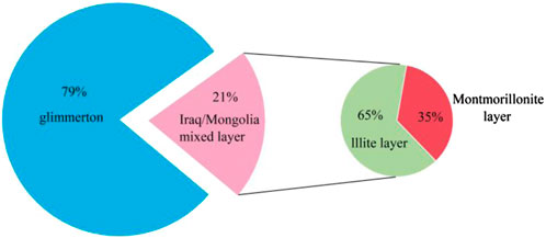
Figure 1. Analysis of clay mineral content, total organic carbon content and maturity.

3.2 Experimental equipment and experimental process

3.2.1 Sample preparation

In order to study anisotropy of bedding shale, a plunger sample measuring 2.5 cm in diameter and 5.0 cm in length was extracted from the rock at angles of 0°, 45° and 90° between the bedding plane and the end face of the rock sample by diamond wire cutting, as shown in Figure 2.

Figure 2

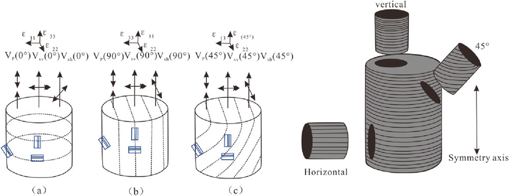
Figure 2. Shale coring azimuth diagram at different angles.

In Figure 2, V_p (0°) denotes the longitudinal wave propagating parallel to the symmetry axis, with its vibration direction aligned with the propagation direction. V_p (45°) represents the longitudinal wave propagating at a 45° angle to the symmetry axis, with its vibration direction coinciding with the propagation direction. V_p (90°) indicates the longitudinal wave propagating perpendicular to the symmetry axis, where the propagation and vibration directions are aligned. V_sh (0°) describes the shear wave traveling parallel to the symmetry axis, with the vibration direction parallel to the bedding plane. V_sh (45°) refers to the shear wave propagating at a 45° angle to the symmetry axis, with the vibration direction perpendicular to the propagation direction. V_sh (90°) illustrates the shear wave propagating perpendicular to the symmetry axis, with the vibration direction parallel to the bedding plane. V_sv (0°) denotes the shear wave propagating parallel to the symmetry axis, with the vibration direction parallel to the bedding plane. V_sv (45°) represents the shear wave propagating at a 45° angle to the symmetry axis, with the vibration direction perpendicular to the propagation direction. V_sv (90°) indicates the shear wave propagating perpendicular to the symmetry axis, with the vibration direction perpendicular to the bedding plane.

3.2.2 Experimental device

This study needs to test the acoustic and mechanical characteristics of rocks at the same time. The instrument in question is a multifunctional rock acoustic and mechanical parameter measuring system (Figure 3), this system is engineered to conduct acoustic and triaxial mechanical experiments on rock samples under reservoir conditions, with temperatures reaching as high as 150°C and pressures up to 68 MPa. When measuring mechanical parameters, apart from pore pressure and confining pressure, it can also produce axial pressure of about 820 kN at most; There are two ways to measure strain: strain gauge or LVDT. The equipment can be operated by manual control, software control and script control, and can be automatically measured. To enhance the precision of radial strain measurement, this test intends to utilize a strain gauge for measuring shale strain.

Figure 3

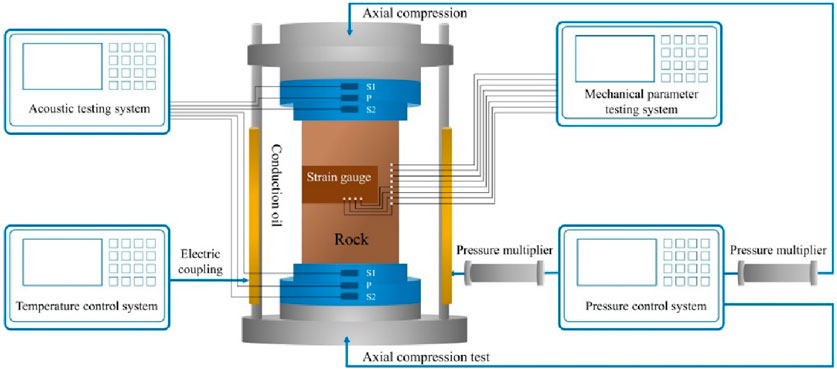
Figure 3. Joint measurement system of rock sample acoustics and mechanics.

The acoustic probe integrates a pair of longitudinal wave transducers and two pairs of orthogonally polarized shear wave transducers, with central frequencies of 0.8 and 0.45 MHz, respectively.

3.2.3 Experimental process

The confining pressure is kept at 30 MPa, and the deviatoric stress is controlled from 0 to carry out nine continuous pressurization/depressurization cycles. Each cycle involves a 5 MPa increase in the maximum deviatoric stress, culminating in a final cycle with a maximum deviatoric stress of 45 MPa. The acoustic and mechanical parameters of rock were measured during the whole experiment, as shown in Figure 4.

Figure 4

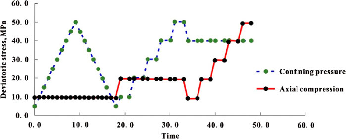
Figure 4. Schematic diagram of rock stress loading path and dynamic and static elastic parameters test.

Response analysis of anisotropy to shale’s dynamic and static elastic properties under cyclic pressure. The variation laws of axial strain, radial strain and volume strain of shale at different angles under different pressurization cycles are analyzed, and the response laws of anisotropy to the nonlinear lag evolution characteristics of rocks are discussed, and the effects of anisotropy on the dynamic and static elastic properties of shale subjected to cyclic pressurization are analyzed in detail.

4 Dynamic elastic parameters and its anisotropy

4.1 Ultrasonic velocity and its anisotropy

Keep the deviatoric stress at 10 MPa, and compare and analyze the P-wave velocity, fast and slow shear wave velocity of rocks at different angles when the confining pressures are 0, 5, 10, 15, 20, 25, 30,35, 40, 45 and 50 MPa, respectively (Figure 5).

Figure 5

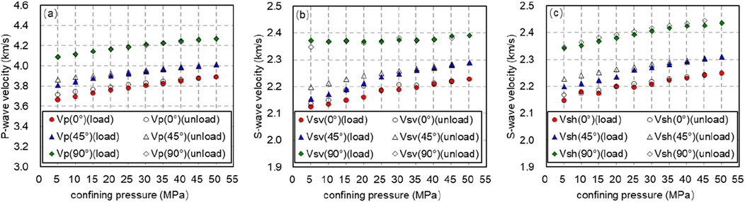
Figure 5. The longitudinal and transverse wave velocities during confining pressure loading (solid line) and unloading (dotted line). (A) The longitudinal wave velocities during confining pressure loading (solid line) and unloading (dotted line). (B) The fast transverse wave velocities during confining pressure loading (solid line) and unloading (dotted line). (C) The slow transverse wave velocities during confining pressure loading (solid line) and unloading (dotted line).

Comparing the velocities of shale samples in different directions, it is found that the velocity of shale satisfies the TI medium $V_{\mathrm{p}}\left({90}^{\circ }\right)>V_{\mathrm{p}}\left({45}^{\circ }\right)>V_{\mathrm{p}}\left(0^{\circ }\right)$ inequality, $V_{\text{sv}}\left({90}^{\circ }\right)>V_{\text{sv}}\left({45}^{\circ }\right)>V_{\text{sv}}\left(0^{\circ }\right)$ and, $V_{\text{sh}}\left({90}^{\circ }\right)>V_{\text{sh}}\left({45}^{\circ }\right)>V_{\text{sh}}\left(0^{\circ }\right)$ which is consistent with the velocity relationship of natural gas shale in different directions in other literatures (Gong et al., 2020). As confining pressure rises, the velocities of P-waves, fast shear waves, and slow shear waves in various bedding orientations also increase. This phenomenon occurs mainly due to the closure of micro-cracks and flexible pores in the shale, leading to enhanced rock stiffness and resulting in faster sound wave propagation.

Comparing the velocities during loading and unloading, it is found that there is a difference between the two processes, that is, the unloading process exhibits a higher acoustic velocity than the loading process. Taking the rock under axial compression of 10 MPa and confining pressure of 50 MPa as an example, during loading, $V_{\mathrm{p}}\left(0^{\circ }\right)$, $V_{\mathrm{p}}\left({45}^{\circ }\right)$, and $V_{\mathrm{p}}\left({90}^{\circ }\right)$ are 3.7777, 3.9225 and 4.1835 km/s respectively; When the pressure is released, the sum is 3.8111, 3.9381 and 4.1902 km/s, respectively, which is consistent with previous studies on the loading and unloading process of shale (Gong F et al., 2019; Wang et al., 2020b). The primary cause of this situation is the irreversible change of rock microstructure. Inelastic pores and micro-cracks are closed during the loading process, and these inelastic pores and micro-cracks cannot be completely recovered during the unloading process, which leads to the difference of acoustic wave velocity during the loading or unloading process.

In the loading phase, as the confining pressure rises from 5 to 50 MPa, $V_{\mathrm{p}}\left(0^{\circ }\right)$ increases by 0.224 km/s, $V_{\mathrm{p}}\left({45}^{\circ }\right)$ and $V_{\mathrm{p}}\left({90}^{\circ }\right)$ increase by 0.2038 and 0.182 km/s. The research findings indicate that there are differences in the growth rates of acoustic velocity across different bedding directions, with the increase in acoustic velocity along the symmetry axis being notably greater than that observed perpendicular to the symmetry axis. And the growth rate of longitudinal wave velocity surpasses that of shear wave velocity.

During the pressurization process, with the confining pressure increasing from 10 to 50 MPa, the P-wave and S-wave velocities of the rock are measured at axial pressures of 10 and 20 MPa, respectively. The results of these tests are illustrated in Figure 6.

Figure 6

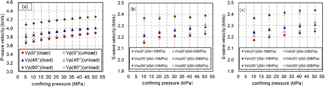
Figure 6. The velocity changes of longitudinal wave and transverse wave in the process of confining pressure. (A) The longitudinal velocity changes of longitudinal wave and transverse wave in the process of confining pressure. (B) The slow transverse wave velocity changes of longitudinal wave and transverse wave in the process of confining pressure. (C) The fast transverse wavevelocity changes of longitudinal wave and transverse wave in the process of confining pressure.

In Figure 6, the solid line corresponds to an axial compression of 10 MPa, whereas the dashed line indicates an axial pressure of 20 MPa. It is evident that, under the same confining and axial pressures, rocks exhibiting various bedding angles show differences in both P-wave and S-wave velocities. $V_{\mathrm{p}}\left({90}^{\circ }\right)>V_{\mathrm{p}}\left({45}^{\circ }\right)>V_{\mathrm{p}}\left(0^{\circ }\right)$ $V_{\text{sv}}\left({90}^{\circ }\right)>V_{\text{sv}}\left({45}^{\circ }\right)>V_{\text{sv}}\left(0^{\circ }\right)$ and $V_{\text{sh}}\left({90}^{\circ }\right)>V_{\text{sh}}\left({45}^{\circ }\right)>V_{\text{sh}}\left(0^{\circ }\right)$ when the axial pressure is constant, both the P-wave velocity and S-wave velocity increase in different bedding directions as the confining pressure rises. The primary cause lies in the increase of confining pressure or axial pressure, micro-cracks and flexible pores in shale are closed, rock stiffness increases and sound wave propagation becomes faster. The acoustic velocity measured along the symmetry axis is notably greater than the rate of increase observed in the direction perpendicular to the symmetry axis, while the growth rate of longitudinal wave velocity surpasses that of transverse wave velocity.

4.2 Dynamic elastic modulus and anisotropy

For VTI media, especially horizontal layered shale, the stress-strain relationship adheres to the generalized Hooke’s law, as shown in Formula 1, Auld (1973).

${\sigma }_{ij}=C_{ijkl}\cdot {\epsilon }_{kl}(1)$

where is ${\sigma }_{ij}$ the stress component; Is ${\epsilon }_{kl}$ the strain component; Is $C_{ijkl}$ the stiffness coefficient matrix, and the specific form is Formula 2.

$\left[\begin{array}{l}{\sigma }_{11}\\ \begin{array}{l}{\sigma }_{22}\\ \begin{array}{l}{\sigma }_{33}\\ {\sigma }_{23}\end{array}\\ {\sigma }_{13}\end{array}\\ {\sigma }_{12}\end{array}\right]=\left[\begin{array}{cccccc}{C}_{11}& C_{12}& C_{13}& 0& 0& 0\\ C_{12}& C_{11}& C_{13}& 0& 0& 0\\ C_{13}& C_{13}& C_{33}& 0& 0& 0\\ 0& 0& 0& C_{44}& 0& 0\\ 0& 0& 0& 0& C_{44}& 0\\ 0& 0& 0& 0& 0& C_{66}\end{array}\right]\left[\begin{array}{l}{\epsilon }_{11}\\ \begin{array}{l}{\epsilon }_{22}\\ \begin{array}{l}{\epsilon }_{33}\\ 2{\epsilon }_{23}\end{array}\\ 2{\epsilon }_{13}\end{array}\\ 2{\epsilon }_{12}\end{array}\right](2)$

The stiffness coefficient matrix of transversely isotropic strata contains five independent stiffness coefficients, namely, C₁₁, C₃₃, C₄₄, C₆₆, and C₁₃. Stiffness coefficient C₁₂ is not an independent parameter, it is closely related to $C_{12}=C_{11}-2C_{66}$ and. These five stiffness coefficients are closely related to formation density and P-wave velocity.

The dynamic stiffness coefficients C_11d, C_33d, C_44d, C_66d, C_12d, and C_13d (Cheadle et al., 1991; Mah and Schmidt. 2001), the specific formula is as follows.

$C_{11\mathrm{d}}={\rho }_{\mathrm{b}}{V}_{\mathrm{p}}^2\left(90°\right)(3)$

$C_{33\mathrm{d}}={\rho }_{\mathrm{b}}{V}_{\mathrm{p}}^2\left(0°\right)(4)$

$C_{66\mathrm{d}}={\rho }_{\mathrm{b}}{V}_{\text{sh}}^2\left(90°\right)(5)$

$C_{44\mathrm{d}}={\rho }_{\mathrm{b}}{V}_{\text{sv}}^2\left(0°\right)(6)$

$C_{12\mathrm{d}}=C_{11\mathrm{d}}-2{\rho }_{\mathrm{b}}{V}_{\text{sh}}^2\left(90°\right)(7)$

$\begin{array}{l}{C}_{13\mathrm{d}}=-C_{44\mathrm{d}}\hfill \\ \hfill & +\sqrt{4{\rho }_{\mathrm{b}}^2{V}_{\mathrm{p}}^4\left(45°\right)-2{\rho }_{\mathrm{b}}{V}_{\mathrm{p}}^2\left(45°\right)\left(C_{11\mathrm{d}}+C_{33\mathrm{d}}+2C_{44\mathrm{d}}\right)+\left(C_{11\mathrm{d}}+C_{44\mathrm{d}}\right)\left(C_{33\mathrm{d}}+C_{44\mathrm{d}}\right)}\hfill \end{array}(8)$

where the longitudinal $V_{\mathrm{p}}\left(0^{\circ }\right)$ wave traveling along the symmetry axis, the direction of vibration aligns with the direction of propagation. For the longitudinal wave $V_{\mathrm{p}}\left({45}^{\circ }\right)$, which propagates at a 45-degree angle to the symmetry axis, the vibration direction also corresponds to the propagation direction. In the case of the longitudinal wave $V_{\mathrm{p}}\left({90}^{\circ }\right)$, propagating perpendicularly to the symmetry axis, the propagation direction matches the vibration direction. Shear wave $V_{\text{sh}}\left(0^{\circ }\right)$, which propagates parallel to the symmetry axis, has a vibration direction that runs parallel to the bedding plane. The transverse wave $V_{\text{sh}}\left({45}^{\circ }\right)$, oriented at a 45-degree angle with respect to the symmetry axis, exhibits a vibration direction that is perpendicular to the propagation path. For the transverse wave $V_{\text{sh}}\left({90}^{\circ }\right)$, which moves perpendicular to the symmetry axis, the vibration direction is aligned with the internal layer structure. The $V_{\text{sv}}\left(0^{\circ }\right)$ transverse wave, propagating parallel to the symmetry axis, also has a vibration direction that is parallel to the interior of the layer. The transverse wave $V_{\text{sv}}\left({45}^{\circ }\right)$, moving at a 45-degree angle to the symmetry axis, has its vibration direction perpendicular to that of the propagation. Finally, the transverse wave $V_{\text{sv}}\left({90}^{\circ }\right)$, traveling perpendicular to the symmetry axis, features a vibration direction that is also perpendicular to the internal layer

According to this, the dynamic Young’s Modulus E_11d and E_33d and the dynamic Poisson’s ratios μ_12d, μ_31d and μ_13d of shale in different directions can be obtained (Christensen and Zywicz, 1990; Gautam and Wong, 2006):

$E_{11\mathrm{d}}=C_{11\mathrm{d}}+\frac{C_{13\mathrm{d}}^2\left(-C_{11\mathrm{d}}+C_{12\mathrm{d}}\right)+C_{12\mathrm{d}}\left(-C_{33\mathrm{d}}{C}_{12\mathrm{d}}+C_{13\mathrm{d}}^2\right)}{C_{33\mathrm{d}}{C}_{11\mathrm{d}}-C_{13\mathrm{d}}^2}(9)$

$E_{33\mathrm{d}}=\frac{C_{11\mathrm{d}}^2{C}_{33\mathrm{d}}+2C_{13\mathrm{d}}^2{C}_{12\mathrm{d}}-2C_{11\mathrm{d}}{C}_{13\mathrm{d}}^2-C_{33\mathrm{d}}{C}_{12\mathrm{d}}^2}{C_{11\mathrm{d}}^2-C_{12\mathrm{d}}^2}(10)$

${\mu }_{12\mathrm{d}}=\frac{C_{33\mathrm{d}}{C}_{12\mathrm{d}}-C_{13\mathrm{d}}^2}{C_{33\mathrm{d}}{C}_{11\mathrm{d}}-C_{13\mathrm{d}}^2}(11)$

${\mu }_{31\mathrm{d}}=\frac{C_{13\mathrm{d}}}{C_{11\mathrm{d}}+C_{12\mathrm{d}}}(12)$

${\mu }_{13\mathrm{d}}=\frac{C_{13\mathrm{d}}\left(C_{11\mathrm{d}}-C_{12\mathrm{d}}\right)}{C_{33\mathrm{d}}{C}_{11\mathrm{d}}-C_{13\mathrm{d}}^2}(13)$

where: is E_11d the dynamic Young’s modulus measured by cores with parallel bedding planes; In order E_33d to use the dynamic Young’s modulus measured by the vertical bedding plane core; μ_12d, μ_13d,is the dynamic Poisson’s ratio measured by cores with parallel bedding planes; μ_31d To utilize the dynamic Poisson’s ratio obtained from cores taken along the vertical bedding plane.

The dynamic stiffness coefficient of rock can be obtained from Formulas 3–8. Figure 7 shows the dynamic stiffness coefficient of rock obtained during pressurization or depressurization when the axial pressure is 10 MPa and the confining pressure changes from 5 to 50 MPa.

Figure 7

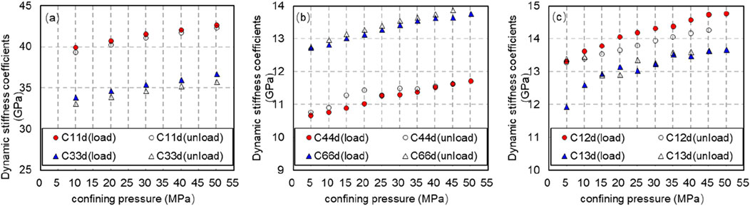
Figure 7. Variation of dynamic stiffness coefficient with confining pressure (axial pressure is 10 MPa, solid line is pressurization process, and dotted line is decompression process). (A) Variation of dynamic stiffness coefficient C11d and C33d with confining pressure (axial pressure is 10 MPa, solid line is pressurization process, and dotted line is decompression process). (B) Variation of dynamic stiffness coefficient C44d and C66d with confining pressure (axial pressure is 10 MPa, solid line is pressurization process, and dotted line is decompression process). (C) Variation of dynamic stiffness coefficient C12d and C13d with confining pressure (axial pressure is 10 MPa, solid line is pressurization process, and dotted line is decompression process).

From Figure 7, it is evident that when the axial pressure remains constant, the dynamic stiffness coefficients C_11d, C_33d, C_44d, C_66d, C_12d and C_13d of rock all increase with the rise of confining pressure during loading or unloading; Under the same confining pressure, the dynamic stiffness coefficient obtained in unloading process is greater than that obtained in loading process.

In the process of pressurization, the axial pressure is controlled to be 10 and 20 MPa, and the confining pressure is raised from 10 to 50 MPa. With the axial pressure held constant, the dynamic stiffness coefficient increases as confining pressure rises. Additionally, at the same confining pressure, the dynamic stiffness coefficient observed with 20 MPa of axial compression is higher than that seen with 10 MPa of axial compression, as illustrated in Figure 8.

Figure 8

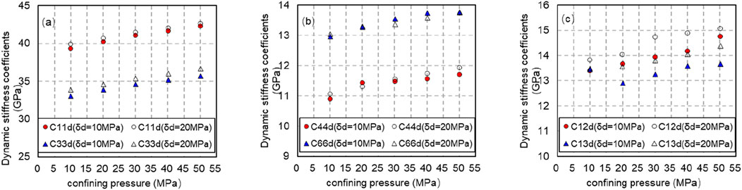
Figure 8. Variation of dynamic stiffness coefficient with confining pressure (solid line shows axial compression of 10 MPa, and dotted line shows axial compression of 20 MPa during pressure relief).(A) Variation of dynamic stiffness coefficient C11d and C33d with confining pressure (solid line shows axial compression of 10 MPa, and dotted line shows axial compression of 20 MPa during pressure relief). (B) Variation of dynamic stiffness coefficient C44d and C66d with confining pressure (solid line shows axial compression of 10 MPa, and dotted line shows axial compression of 20 MPa during pressure relief). (C) Variation of dynamic stiffness coefficient C12d and C13d with confining pressure (solid line shows axial compression of 10 MPa, and dotted line shows axial compression of 20 MPa during pressure relief).

From Formulas 9–13, the dynamic Young’s modulus, dynamic Poisson’s ratio and dynamic stiffness coefficient in different bedding directions can be calculated. Figure 9 depicts the changing trend of dynamic Young’s modulus and dynamic Poisson’s ratio with confining pressure at different bedding angles when the axial pressure is 10 MPa and the confining pressure is increased from 5 to 50 MPa. Figure 9 exhibits Young’s modulus at different bedding angles increases with the increase of confining pressure when the axial pressure is constant. Under the same confining pressure, the dynamic Young’s modulus measured by cores with parallel bedding plane is greater than that measured by cores with vertical bedding plane. At the same bedding angle, the dynamic Young’s modulus obtained during pressure relief is greater than that obtained during pressure increase.

Figure 9

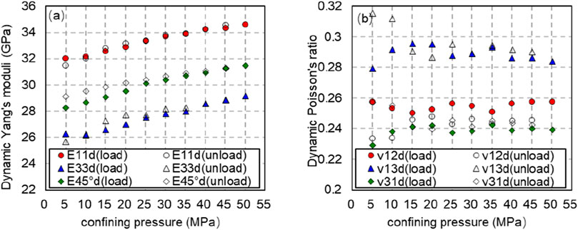
Figure 9. Dynamic Young’s modulus and Poisson’s ratio with confining pressure at different bedding angles. Variation law (solid line is pressurization process, dotted line is depressurization process). (A) Dynamic Young’s modulus with confining pressure at different bedding angles. Variation law (solid line is pressurization process, dotted line is depressurization process). (B) Dynamic Poisson’s ratio with confining pressure at different bedding angles. Variation law (solid line is pressurization process, dotted line is depressurization process).

According to the anisotropy parameter proposed by Thomsen (1986), the anisotropy of shale can be expressed $\epsilon$ by $\gamma$ three $\delta$ independent parameters, sum, as shown in Equations 14–18.

$\alpha =\sqrt{C_{33}/\rho }(14)$

$\beta =\sqrt{C_{44}}(15)$

$\epsilon =\frac{C_{11}-C_{33}}{2C_{33}}(16)$

$\gamma =\frac{C_{66}-C_{44}}{2C_{44}}(17)$

$\delta =\frac{{\left(C_{13}+C_{44}\right)}^2-{\left(C_{33}-C_{44}\right)}^2}{2C_{33}\left(C_{33}-C_{44}\right)}(18)$

where: ε is anisotropy of longitudinal wave velocity, γ is anisotropy of shear wave velocity, and δ is coefficient of variation of longitudinal wave, which indicates the speed of change of anisotropy of longitudinal wave in vertical direction.

From Figure 10, when the axial pressure remains constant, α the β dynamic ε anisotropy γ coefficients δ of rock, and exhibit varying patterns in response to the confining pressure under loading or unloading conditions. When maintaining constant axial pressure, it rises with $\alpha$ the $\beta$ elevation of confining pressure under loading or $\epsilon$ unloading, $\gamma$ and $\delta$ diminishes with escalating confining pressure. At an equal confining pressure, are $\alpha$ basically $\beta$ the $\epsilon$ same during loading and unloading, and the value $\gamma$ of, $\delta$ during loading is greater than that during unloading.

Figure 10

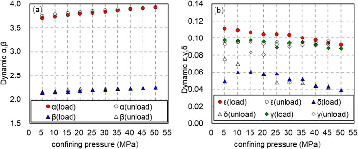
Figure 10. Variation law of dynamic anisotropy coefficient with confining pressure (solid line shows pressurization process and dotted line shows depressurization process). (A) Variation law of dynamic anisotropy coefficient α, β with confining pressure (solid line shows pressurization process and dotted line shows depressurization process). (B) Variation law of dynamic anisotropy coefficient ε, γ and δ with confining pressure (solid line shows pressurization process and dotted line shows depressurization process).

In the process of pressurization, the axial pressure is controlled to be 10 and 20 MPa, and the confining pressure is increased from 10 to 50 MPa. Under the same axial pressure, the dynamic anisotropy $\alpha$ coefficient $\beta$ rises with the escalation of confining pressure, and decreases $\epsilon$ with $\gamma$ the $\delta$ increase of confining pressure. Under the same confining pressure, the anisotropy coefficient under the axial compression of 20 MPa is smaller than the dynamic anisotropy coefficient under the axial compression of 10 MPa, as shown in Figure 11.

Figure 11

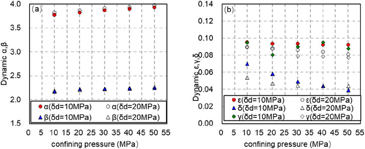
Figure 11. Variation of dynamic anisotropy coefficient with confining pressure (solid line is axial compression of 10 MPa, dashed line is axial compression of 20 MPa). (A) Variation of dynamic anisotropy coefficient α, β with confining pressure (solid line is axial compression of 10 MPa, dashed line is axial compression of 20 MPa). (B) Variation of dynamic anisotropy coefficient t ε, γ and δ with confining pressure (solid line is axial compression of 10 MPa, dashed line is axial compression of 20 MPa).

In the process of increasing pressure, there are at least three mechanisms that will affect the anisotropy of the sample. When the oriented arrangement of clay minerals is enhanced, the corresponding compaction process will reduce the porosity of the sample. The increase of oriented arrangement of clay minerals will increase the anisotropy of the sample velocity, but the decrease of porosity will decrease the anisotropy of the sample, which is due to the size and shape of mineral particles. Under the same stress, larger particles are more likely to be broken than smaller ones. In the process of compaction, “hard” pores may be transformed into “soft” pores arranged neatly, consequently resulting in the escalation of velocity anisotropy. Hence, these mechanisms ought to be taken into account during the shale compaction process.

5 Static elastic parameters and its anisotropy

5.1 Stress-strain curve

The rock samples underwent triaxial compression experiments. The triaxial compression measurement is shown in Figure 12. The three curves in the Fig represent axial strain, radial strain and axial pressure respectively. One static elastic constant measurement is carried out for three pressurization cycles-the axial pressure increases by 15 MPa at a uniform speed, and then decreases to the initial pressure. For three cycles, the axial pressure and axial and radial strains are collected and the static elastic constant of rock samples is calculated, as shown in Figure 13.

Figure 12

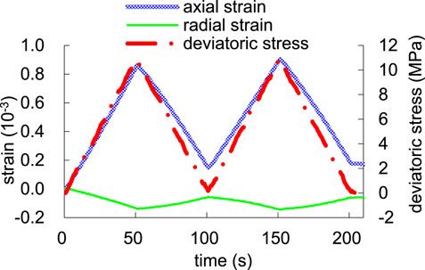
Figure 12. Static elastic parameter measurement process.

Figure 13

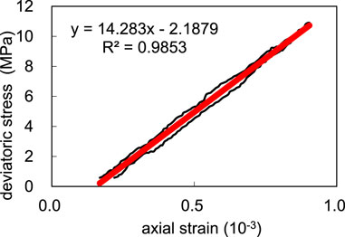
Figure 13. Calculation diagram of static elastic mechanical parameters.

5.2 Static elastic modulus and anisotropy

5.2.1 Static elastic modulus calculation of rock

According to the stress-strain measurement results, the static Young’s modulus E_11s and E_33s of shale and the static Poisson’s ratios μ_12s, μ_31s and μ_13s can be calculated (Cheadle et al., 1991; Mah and Schmitt, 2001; Miller et al., 2013):

$E_{11\mathrm{s}}=\mathrm{\partial }{\sigma }_{11}/\mathrm{\partial }{\epsilon }_{11}(19)$

$E_{33\mathrm{s}}=\mathrm{\partial }{\sigma }_{33}/\mathrm{\partial }{\epsilon }_{33}(20)$

$E_{\mathrm{s}}\left(45°\right)=\mathrm{\partial }\sigma \left(45°\right)/\mathrm{\partial }\epsilon \left(45°\right)(21)$

${\mu }_{12\mathrm{s}}=-\mathrm{\partial }{\epsilon }_{22}/\mathrm{\partial }{\epsilon }_{11}(22)$

${\mu }_{31\mathrm{s}}=-\mathrm{\partial }{\epsilon }_{11}/\mathrm{\partial }{\epsilon }_{33}(23)$

${\mu }_{13\mathrm{s}}=-\mathrm{\partial }{\epsilon }_{33}/\mathrm{\partial }{\epsilon }_{11}(24)$

where: E_11s is the dynamic Young’s modulus obtained through measurement by cores with parallel bedding planes; For the purpose of using the dynamic Young’s modulus of the E_33s direction, which is measured by the vertical bedding plane core; μ_12s, μ_13s is the dynamic Poisson’s ratio measured by cores with parallel bedding planes; μ_31s To utilize the dynamic Poisson’s ratio measured from vertical bedding plane cores. In the pressurization-depressurization cycle, the axial pressure is controlled to be 0∼10 MPa. With the increase of the confining pressure from 10 to 50 MPa, the sum of static Young’s modulus of different bedding angles obtained in both the E_11s pressurization E_33s process $E\left({45}^{\circ }\right)$ and the depressurization process intensifies with the rise in confining pressure. Like the dynamic Young’s modulus, in the depressurization process, the static Young’s modulus of different bedding angles is greater than that in the pressurization process. The change of static Poisson’s ratio with confining pressure at different bedding angles is more complicated, ν_12s but ν_31s it is not obvious with the increase of ν_13s confining pressure, and it decreases significantly with the increase of confining pressure during pressurization or depressurization, as shown in Figure 14.

Figure 14

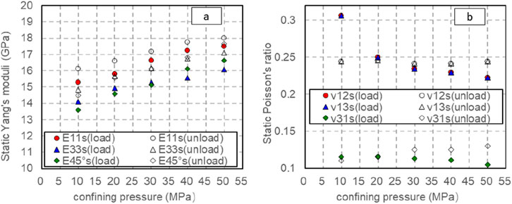
Figure 14. Changes of static elastic parameters with confining pressure at different bedding angles (axial pressure is 0–10 MPa). (A) Changes of static Young’s modulus with confining pressure at different bedding angles (axial pressure is 0–10 MPa). (B) Changes of static Poisson’s ratio with confining pressure at different bedding angles (axial pressure is 0–10 MPa).

5.2.2 Determination of static stiffness coefficient of rock

The stress-strain method can be utilized to ascertain the static elastic modulus of rock. For VTI medium, the static stiffness coefficients C_11s, C_33s, C_44s, C_66s, C_12s and C_13s of shale can be further calculated. The specific formulas are as follows (Wang et al., 2020a):

$C_{11\mathrm{s}}=\frac{E_{11\mathrm{s}}\left(1+{\mu }_{13\mathrm{s}}{\mu }_{31\mathrm{s}}\right)}{\left(1-{\mu }_{12\mathrm{s}}-2{\mu }_{13\mathrm{s}}{\mu }_{31\mathrm{s}}\right)\left(1+{\mu }_{12\mathrm{s}}\right)}(25)$

$C_{33\mathrm{s}}=\frac{E_{33\mathrm{s}}\left(1-{\mu }_{12\mathrm{s}}^2\right)}{\left(1-{\mu }_{12\mathrm{s}}-2{\mu }_{13\mathrm{s}}{\mu }_{31\mathrm{s}}\right)\left(1+{\mu }_{12\mathrm{s}}\right)}(26)$

$C_{44\mathrm{s}}={\left[\frac{4}{E_{\mathrm{s}}\left(45°\right)}-\frac{1}{E_{11\mathrm{s}}}-\frac{1-2{\mu }_{31\mathrm{s}}}{E_{33\mathrm{s}}}\right]}^{-1}(27)$

$C_{66\mathrm{s}}=\frac{E_{11\mathrm{s}}}{2\left(1+{\mu }_{12\mathrm{s}}\right)}(28)$

$C_{12\mathrm{s}}=\frac{E_{11\mathrm{s}}\left({\mu }_{12\mathrm{s}}+{\mu }_{13\mathrm{s}}{\mu }_{31\mathrm{s}}\right)}{\left(1-{\mu }_{12\mathrm{s}}-2{\mu }_{13\mathrm{s}}{\mu }_{31\mathrm{s}}\right)\left(1+{\mu }_{12\mathrm{s}}\right)}(29)$

$C_{13\mathrm{s}}=\frac{E_{11\mathrm{s}}{\mu }_{31\mathrm{s}}}{1-{\mu }_{12\mathrm{s}}-2{\mu }_{13\mathrm{s}}{\mu }_{31\mathrm{s}}}(30)$

The static stiffness coefficient of rock can be obtained from Formulas 25–30. Figure 15 shows the static stiffness coefficient of rock obtained during pressurization or depressurization when the axial pressure is 0–10 MPa and the confining pressure changes from 5 to 50 MPa.

Figure 15

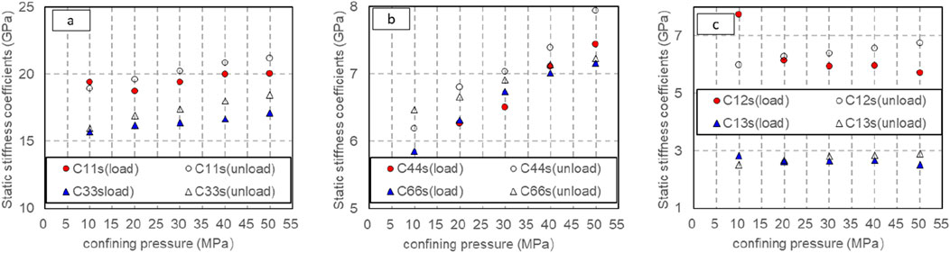
Figure 15. Variation of static stiffness coefficient with confining pressure (solid line pressurization process, dotted line decompression process). (A) Variation of static stiffness coefficient C11s, C33s with confining pressure (solid line pressurization process, dotted line decompression process). (B) Variation of static stiffness coefficient C44s, C66s with confining pressure (solid line pressurization process, dotted line decompression process). (C) Variation of static stiffness coefficient C12s, C13s with confining pressure (solid line pressurization process, dotted line decompression process).

Figure 15 illustrates that the static stiffness coefficients C_11s, C_33s, C_44s, C_66s, C_12s and C_13s of rock exhibit an increment as the confining pressure rises during loading or unloading; Under the same confining pressure, the static stiffness coefficient obtained in unloading process is greater than that obtained in loading process. The static stiffness coefficients C_44s and C_66s, exhibit significant variations with the escalating confining pressure during pressurization or depressurization, whereas C_11s, C_33s and C_13s remain unaffected by the changing confining pressure levels. During pressurization, C_12s declines as the confining pressure rises, while during depressurization, it escalates alongside the increasing confining pressure.

Equations 14–18 offer a method for computing the static anisotropy characteristics of shale oil specimens. Observation from Figure 16 reveals that the anisotropy parameter obtained during the pressure relief process is greater than that obtained during the pressurization process. ε With γ the increase of confining pressure, anisotropy value decreases slightly, and the parameters obtained in pressurization stage and decompression stage have no obvious change law with confining pressure.

Figure 16

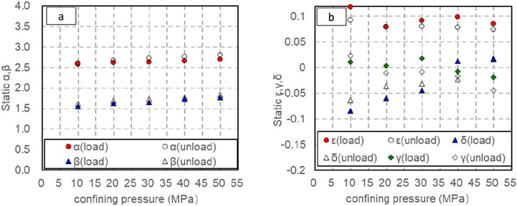
Figure 16. Variation of static anisotropy coefficient α, β with confining pressure (solid line shows pressurization process and dotted line shows depressurization process). (A) Variation of static anisotropy coefficient α, β with confining pressure (solid line shows pressurization process and dotted line shows depressurization process). (B) Variation of static anisotropy coefficient ε, γ and δ with confining pressure (solid line shows pressurization process and dotted line shows depressurization process).

6 Comparative analysis of dynamic and static elastic parameters

Contrast and analyze the dynamic Young’s modulus and static Young’s modulus measured during loading or unloading under the experimental conditions of confining pressure of 1–50 MPa and eccentric stress of 10 MPa (Figure 17). From Figure 7, it is observable that the dynamic and static Young’s moduli increase as the confining pressure rises. The Young’s modulus in different directions is higher than that in the pressurized state, given the same confining pressure. Taking into account the impact of confining pressure, the model for converting dynamic and static Young’s Modulus in various orientations (Table 3) reveals a notable relationship between the static Young’s Modulus in distinct directions and the dynamic Young’s Modulus in the corresponding direction post pressure adjustment. Through the model conversion outlined in Table 3, the application domain can be extended to vertical, horizontal, and high-angle wells, thereby enabling the accurate determination of the static mechanical parameters of rocks under various well-logging conditions.

Figure 17

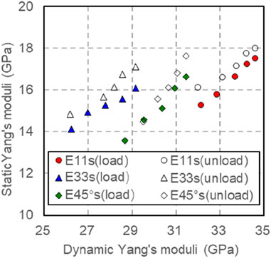
Figure 17. Dynamic and Static elastic modulus under different confinement pressure and pressure.

Table 3

Table 3. Dynamic and static Young’s modulus conversion models in different directions.

Considering the dynamic and static elastic modulus conversion model in different directions (see Figure 18), the static Young’s modulus that has been calculated correlates well with the measured static Young’s modulus, and the correlation coefficient is 0.9268 (see Fig 18). Using this conversion model, the static Young’s modulus of rocks in different directions can be predicted under arbitrary pressure.

Figure 18

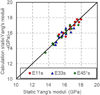
Figure 18. Dynamic and static Young’s relief conditions modulus conversion model.

The dynamic Poisson’s ratio and Poisson’s ratio are measured during loading or unloading under the experimental conditions of confining pressure of 10–50 MPa and eccentric stress of 10 MPa (Figure 19). Upon examining Figure 19, it becomes evident that under pressure relief, the change in ν_12s with respect to confining pressure is not significant, whereas under pressure, ν_12s decreases as the confining pressure increases. Under the pressure ν_31s relief condition, the change of confining pressure is not obvious, but ν_31s it decreases with the increase of confining ν_13s pressure under the pressure condition. It is insensitive to the relationship with confining pressure under the condition of pressurization or depressurization. Considering the influence of confining pressure, as seen in Table 1, the dynamic and static Poisson’s ratio conversion models in different directions (Table 4) show that the static Poisson’s ratio in different directions after pressure correction has significant correlation with the dynamic Poisson’s ratio in the corresponding direction. Using this conversion model, the static Poisson’s ratio of rocks in different directions under arbitrary pressure can be predicted, as shown in Figure 20.

Figure 19

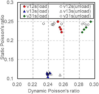
Figure 19. Dynamic and static Poisson’s ratio under different confining pressures and pressure relief conditions.

Table 4

Table 4. Dynamic and static Poisson’s ratio conversion models in different directions.

Figure 20

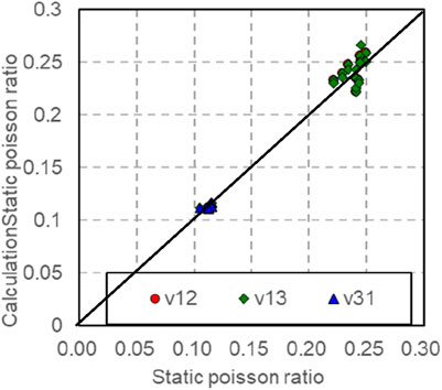
Figure 20. Dynamic and static Poisson’s ratio conversion model.

7 Discussion

Static elastic mechanics parameters is a key parameter in shale oil and gas extraction and water injection fracturing engineering, and different pressurization methods and pressurization conditions have an important influence on the dynamic and static elastic characteristics of shale, so exploring the main controlling factors of the dynamic and static elastic characteristics under different temperature and pressure conditions is a key scientific problem that needs to be solved urgently in shale oil and gas extraction and water injection fracturing engineering.

The acoustic-mechanical coupling system of rock samples was used to analyze the effects of dynamic and static elastic properties of shale at different angles under triaxial pressurization conditions. In order to explore the anisotropy of laminated shale, diamond wire cutting was utilized to cut the rock into three angle samples with the angles of 0 o, 45o and 90 o between the laminated surface and the end face of the rock samples, and the longitudinal wave velocity, as well as the fast and slow transverse wave velocities, were tested for each sample under different temperatures and pressures respectively, and the stress-strain curves of the rock were tested at the same time. Calculation of dynamic stiffness coefficients C11d, C33d, C44d, C66d, C12d, and C13d for different test conditions based on Hooke’s law for VTI media and based on Equations 3–8, and the elastic moduli E11d , E33d, μ12d, μ31d and μ13d were calculated based on the elasticity of different laminar angles based on Equations 9–13. Strain curves, the static modulus of elasticity E11s, E33s, μ12s, μ31s, μ13s are calculated for different lamination angles based on Equations 19–24, based on which the static stiffness coefficients C11s, C33s, C44s, C66s, C12s and C13s can be further calculated.

When calculating the dynamic elasticity parameters, the effects of temperature and pressure need to be taken into account. The dynamic Young’s modulus and static Young’s modulus of shale oil with different stratigraphic angles increase with the increase of pressure, and increase quickly with the pressure when the pressure is lower, and with the continuous increase of pressure, the increase of Young’s modulus slows down and tends to a stable value. The dynamic and static Young’s modulus of shale oil with different stratification angles are linearly related, and the dynamic Young’s modulus is larger than the static Young’s modulus, and the correlation between the dynamic and static Poisson’s ratio is poor, and the dynamic Poisson’s ratio of shale oil is larger than the static Poisson’s ratio in general. There is a strong dependence between the shale oil stiffness coefficient and the perimeter pressure, and the elastic stiffness coefficient shows a trend of increasing with the increase of the perimeter pressure under both dynamic and static test conditions, and the elastic parameters related to longitudinal waves (C11, C33) are more obvious than the elastic parameters related to transverse waves (C44, C66) with the change of pressure. Whether static or dynamic elastic modulus, there are some differences in Young’s modulus and Poisson’s ratio between vertical and horizontal directions, and generally the elastic modulus is larger in the direction of horizontal strata. The Poisson’s ratio/Young’s modulus ratio on different stratigraphy have high correlation, and the Poisson’s ratio/Young’s modulus ratio obtained by acoustic wave test has higher correlation.

The conversion models of Young’s modulus and Poisson’s ratio for different laminar angles were established respectively, which can be applied in vertical wells in vertical wells respectively, and can obtain continuous static elastic mechanical parameters, which extends the adaptability of static rock mechanical parameters.

8 Conclusion and suggestions

Taking the shale oil sample of lacustrine facies in the second member of Kongdong sag in Bohai Bay Basin as the research object, dynamic and static rock acoustics and mechanics were jointly measured in various directions, subsequent examination of the experimental findings culminates in the following deductions:

(1) Under identical confining and axial pressure, the P-wave velocity and S-wave velocity of rocks vary with different bedding angles, and when $V_{\mathrm{p}}\left({90}^{\circ }\right)>V_{\mathrm{p}}\left({45}^{\circ }\right)>V_{\mathrm{p}}\left(0^{\circ }\right)$ the $V_{\text{sv}}\left({90}^{\circ }\right)>V_{\text{sv}}\left({45}^{\circ }\right)>V_{\text{sv}}\left(0^{\circ }\right)$ axial $V_{\text{sh}}\left({90}^{\circ }\right)>V_{\text{sh}}\left({45}^{\circ }\right)>V_{\text{sh}}\left(0^{\circ }\right)$ pressure is constant, the P-wave velocity and S-wave velocity elevate as the confining pressure escalates across different bedding orientations; When the confining pressure remains constant, the velocities of longitudinal and transverse waves in different bedding directions increase with its escalation; The primary factor is that As the confining pressure or axial stress rises, micro-cracks and flexible pores within shale close, rock stiffness increases and sound wave propagation becomes faster. The acoustic velocity aligned with the symmetry axis shows a significantly higher growth rate compared to the velocity observed perpendicular to it, and the growth rate of longitudinal wave velocity exceeds that of transverse wave velocity.

(2) There are differences in dynamic and static Young’s modulus, Poisson’s ratio and stiffness properties in different bedding directions. When maintaining constant axial pressure, the dynamic and static Young’s modulus of different bedding angles rise proportionally with increasing confining pressure. Under the same confining pressure, the dynamic Young’s modulus measured by cores with parallel bedding plane is greater than that measured by cores with vertical bedding plane. At the same bedding angle, the dynamic Young’s modulus recorded during pressure release surpasses that obtained during pressure augmentation. The static young’s modulus and sum of E_11s different E_33s bedding $E\left({45}^{\circ }\right)$ angles increase with rising confining pressure. Like the dynamic young’s modulus, the static young’s modulus of different bedding angles exceeds that of the pressurized one during the process of pressure relief. The alteration of static Poisson’s ratio with varying confining stress across distinct bedding angles presents a more intricate scenario, ν_12s but ν_31s it is not obvious with rising ν_13s confining pressure, and it decreases significantly during both pressurization and depressurization.

(3) The dynamic and static electromechanical properties of different stratigraphic angles can be converted under different pressures, and the dynamic electromechanical parameters measured under different peripheral pressures can be converted into static electromechanical parameters under the corresponding peripheral pressures, which can serve as the foundation for examining the mechanical characteristics of rocks under reservoir conditions, and provide the reference basis for developing a hydraulic fracturing construction program of oil and gas reservoirs.

Data availability statement

The original contributions presented in the study are included in the article/supplementary material, further inquiries can be directed to the corresponding author.

Author contributions

DZ: Writing–review and editing. YL: Data curation, Formal analysis, Writing–review and editing. YG: Investigation, Writing–review and editing. HX: Data curation, Software, Writing–review and editing. YL: Methodology, Supervision, Writing–review and editing. JY: Conceptualization, Investigation, Writing–review and editing. FW: Writing–original draft, Writing–review and editing. YW: Validation, Investigation, Funding acquisition, Writing–review and editing.

Funding

The author(s) declare that financial support was received for the research, authorship, and/or publication of this article. This study was supported by Natural Science Foundation of Shaanxi Provincial Department of Education Upper Level Fund Project (2022JM-139).

Conflict of interest

Authors DZ, YL, YG, HX, YL and JY were employed by Qinghai Oilfeld Company, PetroChina.

The remaining authors declare that the research was conducted in the absence of any commercial or financial relationships that could be construed as a potential conflict of interest.

Generative AI statement

The author(s) declare that no Generative AI was used in the creation of this manuscript.

Publisher’s note

All claims expressed in this article are solely those of the authors and do not necessarily represent those of their affiliated organizations, or those of the publisher, the editors and the reviewers. Any product that may be evaluated in this article, or claim that may be made by its manufacturer, is not guaranteed or endorsed by the publisher.

References

Ameen, M. S., Smart, B. G. D., Somerville, J. M., Hammilton, S., and Naji, N. A. (2009). Predicting rock mechanical properties of carbonates from wireline logs (A case study: arab-D reservoir, Ghawar field, Saudi Arabia). Mar. and Petroleum Geol. 26 (4), 430–444. doi:10.1016/j.marpetgeo.2009.01.017

CrossRef Full Text | Google Scholar

Asef, M. R., and Farrokhrouz, M. (2010). Governing parameters for approximation of carbonates UCS. Electron J. Geotech. Eng. 15, 1581–1592.

Google Scholar

Asef, M. R., and Farrokhrouz, M. (2017). A semi-empirical relation between static and dynamic elastic modulus. J. Petroleum Sci. Eng. 157 (2017), 359–363. doi:10.1016/j.petrol.2017.06.055

CrossRef Full Text | Google Scholar

Auld, B. A. (1973). Acoustic fields and waves in solids. John Wiley and Sons I. doi:10.1063/1.3128926

CrossRef Full Text | Google Scholar

Batzle, M. L., Han, D. H., and Hofmann, R. (2006). Fluid mobility and frequency-dependent seismic velocity—direct measurements. Geophysics 71 (1), N1–N9. doi:10.1190/1.2159053

CrossRef Full Text | Google Scholar

Bian, H. Y., Wang, F., Zhang, C. E., Gao, X. H., ZhangY, H., Duan, C. W., et al. (2019). A new model between dynamic and static elastic parameters of shale based on experimental studies. Arabian J. Geosciences 12 (20), 609. doi:10.1007/s12517-019-4777-2

CrossRef Full Text | Google Scholar

Bian, H. Y., Wang, F., Zhang, Y. H., and Yue, C. W. (2015). Experimental study of dynamic and static elastic parameters of tight sandstones under reservoir conditions. Chin. J. Rock Mechan. Enginee. 34 (S1), 3045–3054. doi:10.13722/j.cnki.jrme.2014.1109

CrossRef Full Text | Google Scholar

Cheadle, S. P., Brown, R. J., and Lawton, D. C. (1991). Orthorhombic anisotropy: a physical seismic modeling study. Geophysics 56 (10), 1603–1613. doi:10.1190/1.1442971

CrossRef Full Text | Google Scholar

Cheng, C. H., and Johnston, D. H. (1981). Dynamic and static moduli. Geophys. Res. Lett. 8 (1), 39–42. doi:10.1029/GL008i001p00039

CrossRef Full Text | Google Scholar

Christensen, R. M., and Zywicz, E. (1990). A three-dimensional constitutive theory for fiber composite laminated media. J. Appl. Mech. 57, 948–955. doi:10.1115/1.2897666

CrossRef Full Text | Google Scholar

Eissa, E. A., and Kazi, A. (1988). Relation between static and dynamic young's moduli of rocks. Int. J. Rock Mech. Min. Sci. and Geomechanics Abstr. 25 (6), 479–482. doi:10.1016/0148-9062(88)90987-4

CrossRef Full Text | Google Scholar

Fjær, E. (2019). Relations between static and dynamic moduli of sedimentary rocks. Geophys. Prospect. 67 (1), 128–139. doi:10.1111/1365-2478.12711

CrossRef Full Text | Google Scholar

Gautam, R., and Wong, R. C. K. (2006). Transversely isotropic stiffness parameters and their measurement in Colorado shale. Can. Geotechnical J. 43 (12), 1290–1305. doi:10.1139/T06-083

CrossRef Full Text | Google Scholar

Ghafoori, M., Rastegarnia, A., and Lashkaripour, G. R. (2018). Estimation of static parameters based on dynamical and physical properties in limestone rocks. J. Afr. Earth Sci. 137 (2018), 22–31. doi:10.1016/j.jafrearsci.2017.09.008

CrossRef Full Text | Google Scholar

Gong, F., Di, B., Wei, J., Ding, P., Tian, H., and Han, J. (2019). A study of the anisotropic static and dynamic elastic properties of transversely isotropic rocks. Geophysics 84 (6), C281–C293. doi:10.1190/geo2018-0590.1

CrossRef Full Text | Google Scholar

Gordon, R. B., and Davis, L. A. (1968). Velocity and attenuation of seismic waves in imperfectly elastic rock. J. Geophys. Res. 73 (12), 3917–3935. doi:10.1029/jb073i012p03917

CrossRef Full Text | Google Scholar

Hornby, B. E., Schwartz, L. M., and Hudson, J. A. (1994). Anisotropic effective-medium modeling of the elastic properties of shales. Geophysics 59 (10), 1570–1583. doi:10.1190/1.1443546

CrossRef Full Text | Google Scholar

Li, H., Han, D. H., Gao, J., Yuan, H., and Wang, Y. (2019). Pressure loading histories and clay fraction effects on the static and dynamic elastic properties of sand-clay synthetic sediments. Powder Technol. 345, 804–814. doi:10.1016/j.powtec.2019.01.033

CrossRef Full Text | Google Scholar

Mah, M., and Schmitt, D. R. (2001). Experimental determination of the elastic coefficients of an orthorhombic material. Geophysics 66 (4), 1217–1225. doi:10.1190/1.1487068

CrossRef Full Text | Google Scholar

Miller, D., Plumb, R., and Boitnott, G. (2013). Compressive strength and elastic properties of a transversely isotropic calcareous mudstone. Geophys. Prospect. 61, 315–328. doi:10.1111/1365-2478.12031

CrossRef Full Text | Google Scholar

Rickman, R., Mullen, M. J., Petre, J. E., Grieser, B., and Kundert, D. (2008). A practical use of shale petrophysics for stimulation design optimization: all shale plays are not clones of the Barnett Shale. SPE Annu. Tech. Conf. Exhib. doi:10.2118/115258-MS

CrossRef Full Text | Google Scholar

Sayers, C. M. (1999). Stress-dependent seismic anisotropy of shales. Geophysics 64 (1), 93–98. doi:10.1190/1.1444535

CrossRef Full Text | Google Scholar

Sone, H., and Zoback, M. D. (2013). Mechanical properties of shale-gas reservoir rocks—Part 1: static and dynamic elastic properties and anisotropy. Geophysics 78 (5), D381–D392. doi:10.1190/geo2013-0050.1

CrossRef Full Text | Google Scholar

Thomsen, L. (1986). Weak elastic anisotropy. Geophysics 51 (10), 1954–1966. doi:10.1190/1.1442051

CrossRef Full Text | Google Scholar

Tutuncu, A. N., Podio, A. L., and Sharma, M. M. (1998). Nonlinear viscoelastic behavior of sedimentary rocks, Part II: hysteresis effects and influence of type of fluid on elastic moduli. Geophysics 63 (1), 195–203. doi:10.1190/1.1444313

CrossRef Full Text | Google Scholar

Vernik, L., and Liu, X. (1997). Velocity anisotropy in shales: a petrophysical study. Geophysics 62 (2), 521–532. doi:10.1190/1.1444162

CrossRef Full Text | Google Scholar

Wang, Y., Han, D. H., Li, H., Zhao, L., Ren, J., and Zhang, Y. (2020a). A comparative study of the stress-dependence of dynamic and static moduli for sandstones. Geophysics 85 (4), MR179–MR190. doi:10.1190/geo2019-0335.1

CrossRef Full Text | Google Scholar

Wang, Y., Zhao, L., Han, D. H., Mitra, A., Li, H., and Aldin, S. (2020b). Anisotropic dynamic and static mechanical properties of organic-rich shale: the influence of stress. Geophysics 86 (2), C51–C63. doi:10.1190/geo2020-0010.1

CrossRef Full Text | Google Scholar

Zhang, L., Ba, J., and Carcione, J. M. (2021). Wave propagation in infinituple-porosity media. J. Geophys. Res. Solid Earth 126 (4), e2020JB021266. doi:10.1029/2020jb021266

CrossRef Full Text | Google Scholar

Zhang, L., Ba, J., Li, C., Carcione, J., and Zhou, F. (2022). Joint inversion of the unified pore geometry of tight sandstones based on elastic and electrical properties. J. Petroleum Sci. Eng. 219, 111109. doi:10.1016/j.petrol.2022.111109

CrossRef Full Text | Google Scholar