Optimization of multi-element geochemical anomaly recognition in the Takht-e Soleyman area of northwestern Iran using swarm-intelligence support vector machine

Mineral exploration is becoming increasingly challenging because the depths at which undiscovered mineral deposits can be found are progressively increasing under barren cover. Therefore, detecting metal resources under barren cover is a significant step for industrial progress. The application of optimized machine learning algorithms is critical for detecting undiscovered deposits under barren cover. One of the most significant issues in mineral exploration is the detection of multi-element geochemical anomalies that could indicate the presence of undiscovered mineral deposits under barren cover. Recently, many machine learning approaches have been developed and employed to model and map multi-element geochemical anomalies, where the important hyperparameters are generally regulated through trial-and-error processes. However, employing swarm-intelligence optimization techniques can reduce the training time and assists with obtaining more precise results. In the present study, a known swarm-intelligence procedure called grasshopper optimization algorithm was implemented to optimize the known hyperparameters of support vector machine (SVM) for identifying multi-element geochemical anomalies in the Takht-e Soleyman district of northwest Iran. The grasshopper-optimized support vector machine was proven to be a rigorous approach for detecting multi-element geochemical anomalies and can also be extended to other geoscientific applications. An optimized SVM algorithm was developed herein using polynomial and radial basis kernel functions that resulted in multi-element geochemical anomaly models with accuracies exceeding 95% in the shortest possible time without trial-and-error approaches.

1 Introduction

The complexity and diversity of geological structures have influenced geochemical signatures related to mineral deposits (Carranza, 2008; Cheng et al., 2000; Sabbaghi et al., 2024). Hence, selecting a suitable machine learning (ML) model for classifying geochemical data into reliable categories is one of the basic steps in mineral prospectivity mapping (MPM) (Ghezelbash et al., 2020; Sabbaghi and Tabatabaei, 2022). Classification techniques employing various traditional ML algorithms are gradually becoming obsolete (Sabbaghi and Tabatabaei, 2020, 2023a, 2023b). ML approaches are extremely useful in different fields owing to their high competency in extracting high-level information from geochemical data. Most ML approaches can be generally categorized into unsupervised and supervised models. Supervised ML models include artificial neural networks (Hinton et al., 2006), deep belief networks (LeCun et al., 2015), convolutional neural networks (LeCun et al., 2015), ensemble learning (Anderson, 1972), random forest (Dietterich, 2002), logistic regression (Cox, 1958), and support vector machines (SVM) (Vapnik, 1999), which are focused on classifying features based on predefined labels. Unsupervised methods recognize the hidden features of unlabeled inputs and include algorithms for density estimation (Scott and Knott, 1974), dimension reduction (Redlich, 1993), feature extraction (Coates et al., 2011), and clustering.

ML algorithms are more robust than traditional classification approaches because they (i) convert the relationships between the inputs and outputs into a representation, (ii) fulfill complex predictions without supposition of data patterns, and (iii) expose new unpredicted structures, patterns, and relationships. Some supervised ML models were recently explored for MPM to detect mineralization occurrences that are inherently associated with great uncertainties and excessive costs (Sabbaghi and Tabatabaei, 2023b). However, ML algorithms can be made more effective with appropriate optimization of their structures. The SVM is a robust and practical approach that can be reinforced through appropriate optimization algorithms. The SVM algorithm includes known hyperparameters, for which users commonly obtain ideal values via trial-and-error procedures. These trial-and-error processes cannot be used for reliable mineral exploration targeting. Hence, users commonly prefer to apply linear kernel functions without tuning the kernel scale or polynomial-order parameters of the SVM (Sabbaghi and Moradzadeh, 2018). Accordingly, application of the radial basis function (RBF) and polynomial function (PF) kernels has mostly resulted in more accurate conclusions (Abedi et al., 2012; Zuo and Carranza, 2011).

Recently, swarm-intelligence optimization algorithms have been introduced for optimization of ML algorithms applied in medical, industrial, agricultural, and geoscientific fields. In fact, swarm-based optimization algorithms have been widely employed owing to their nature-inspired characteristics, which allow consideration of problems as black boxes with great avoidance of local optima, gradient-free mechanisms, and simplicity (Saremi et al., 2017). The grasshopper optimization algorithm (GOA) is a strong swarm-intelligence optimization technique that has been used alongside genetic algorithm (GA) and particle swarm optimization (PSO) (Saremi et al., 2017). Optimization algorithms are commonly selected based on the following criteria: 1) which hyperparameter of an ML model needs to be optimized and 2) should that hyperparameter be maximized or minimized. Accordingly, the SVM as an ML model was selected because of its simplicity, popularity, and computational attractiveness. Furthermore, the GOA was chosen for hybridization with SVM. Then, two hyperparameters of the RBF-SVM and PF-SVM were optimized using the GOA, and their accuracies were compared. Although the accuracies of both optimized models were above 95%, the optimized PF-SVM had greater accuracy.

2 Geology and mineralization

The Takht-e Soleyman area is an important segment of the Takab mineralization zone in northwest Iran; it is located between the Sanandaj-Sirjan Zone (SSZ) and Urumieh-Dokhtar Magmatic Belt (UDMB) within 47°0′0˝ E and 47°30′0˝ E longitudes and 36°30′0˝ N and 37°0′0˝ N latitudes (Figure 1). Its extensional faults display northeast–southwest or east–west trends. This area includes carlin-type gold, epithermal gold, and Mississippi valley type (MVT) Pb–Zn mineralizations (Sabbaghi and Tabatabaei, 2023c). The common rock types in the Takht-e Soleyman area are sedimentary, metamorphic, and carbonate units, while volcanic occurrences are rarely seen. The passive margin settings are the best locations for the formation of MVT Pb–Zn resources as large and continuous stratiform orebodies. These deposits are weakly related to silicification and dolomitization (Wei et al., 2020). The MVT Pb–Zn resources provide over 20% of the global requirements of the elements Pb and Zn. Hence, these resources are highly sought in mineral exploration activities. Carbonated rocks such as limestone and dolostone that are commonly found in foreland basins of orogenic belts are suitable hosts for the formation of these resources (Wei et al., 2020). The main associated minerals of MVT Pb–Zn mineralization include sphalerite, Fe sulfides, and galena (Hosseini-Dinani and Aftabi, 2016). The elements Pb, Zn, Ag, and Cd demonstrate great correlations with Pb–Zn mineralization occurrences in the study area, and a deep-learning framework presented by Sabbaghi and Tabatabaei (2023c) was employed to confirm these elements as pathfinders in the study area. Hence, the geochemical data table of these elements was applied to train the model presented in this work.

Figure 1

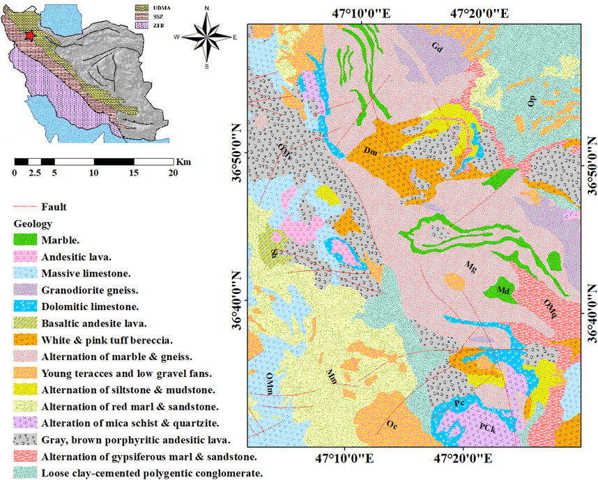
Figure 1. Simplified geological map (1:100,000) of the Takht-e Soleyman area in northwest Iran.

3 Methodology

3.1 SVM algorithm

This ML model includes heuristic algorithms based on statistics (Abedi et al., 2012; Geranian et al., 2016; Gonbadi et al., 2015; Maepa et al., 2021). A dataset of vectors (training data) with predefined (priori knowledge) class labels is commonly used to design the SVM hyperplane for delineating classes (Geranian et al., 2016). This approach employs different kernel functions for transferring the training data to a higher-dimension space (Abedi et al., 2012). A support vector in the SVM method represents a point that has the least distance from the hyperplane and regulates the orientation of the hyperplane (Figure 2). The decision boundary of the hyperplane is commonly determined using a number of input features. The two-class SVM entails training data with l feature vectors, where x_i ∈ R and i = (1, …, n) is the number of the feature vector in the training data. The class label y_i is assigned to each sample and is equal to 1 or −1 (Zuo and Carranza, 2011). The separating hyperplane is formulated as the following decision function:

$f\left(x\right)=sgn\left(wx+b\right),(1)$

where parameters w and b are optimized using the following equation:

$L\left(w,b,\alpha \right)=\frac{1}{2}{‖w‖}^2-{\displaystyle \sum _{i=1}^l}{\alpha }_i\left(y_i\left(\left(x_{i}w\right)+b\right)-1\right).(2)$

Here, ${\alpha }_i$ is the Lagrange multiplier. The Lagrange function is minimized with respect to w and b and maximized with respect to ${\alpha }_i$ > 0. The Lagrange multipliers are determined as follows:

$Maximize{\displaystyle \sum _{i=1}^l}{\alpha }_i-\frac{1}{2}{\displaystyle \sum _{i,j=1}^l}{\alpha }_i{\alpha }_j{y}_i{y}_j\left(x_i{x}_j\right).(3)$

Figure 2

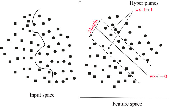
Figure 2. Dataset of vectors (training data) and hyperplanes for discriminating classes in the support vector machine (SVM) approach.

Next, the classification based on the optimal hyperplane is obtained using the following decision function:

$f\left(x\right)=sgn\left({\displaystyle \sum _{i=1}^l}{y}_i{\alpha }_i\left(x{x}_i\right)+b\right).(4)$

Positive slack variables ${\xi }_i$ along with a penalty value C for misclassification errors are considered to improve the classification. Accordingly, the following objective function should be minimized:

$S=\frac{1}{2}{‖w‖}^2+C{\left({\displaystyle \sum _{i=1}^l}{\xi }_i\right)}^k.(5)$

When the training data are not linearly separable, an RBF kernel $K\left(x_i,x_j\right)$ is employed to transfer the training data to the Hilbert space. Then, Equations 3, 4) can be reformulated as follows:

$Maximize{\displaystyle \sum _{i=1}^l}{\alpha }_i-\frac{1}{2}{\displaystyle \sum _{i,j=1}^l}{\alpha }_i{\alpha }_j{y}_i{y}_{j}K\left(x_i{x}_j\right).(6)$

$f\left(x\right)=sgn\left({\displaystyle \sum _{i=1}^l}{y}_i{\alpha }_{i}K\left(x{x}_i\right)+b\right).(7)$

In addition to the RBF kernel, the PF kernel was applied to the SVM model in this study and is expressed as follows:

$K\left(x_i,x_j\right)={\left(x_i{x}_j+1\right)}^d.(8)$

Then, the relevant parameters like the kernel size (σ) of the RBF, kernel order (d) of the PF, and objective function parameter (penalty value C) for both kernels must be optimized for credible results.

3.2 GOA

Grasshoppers are generally observed individually but belong to one of the largest swarm of creatures. Exploitation and exploration of the search space are the two logical attitudes of most nature-inspired optimization algorithms. Here, the search agents are supported for sudden movements in the exploration tendency and local movements in the exploitation tendency. Grasshoppers naturally demonstrate these two tendencies to seek their targets. Therefore, mathematical modeling of their behaviors has been used to construct a new nature-inspired algorithm (Saremi et al., 2017). The simulated behaviors of grasshoppers can be expressed as follows:

$Y_i=P_i+S_i+W_{i,}(9)$

where W_i, P_i, S_i, and Y_i refer to the wind advection, gravity intensity, social interaction, and position of the ith grasshopper, respectively. Moreover, their random behavior can be expressed as Y_i = r₁P_i + r₂S_i + r₃W_i, where r₃, r₂, and r₁ are random values in [0, 1]. The social interaction (S_i) can be calculated as follows:

$S_i={\displaystyle \sum _{j=1}^N}s\left(d_{ij}\right){ď}_{ij}\left(\mathrm{j}\ne \mathrm{i}\right),(10)$

where d_ij is the distance between the ith and jth grasshoppers computed as d_ij =|x_j − x_i|, N is the number of grasshoppers, and s is the strength of social forces depicted as a function and determined using Equation 11. Moreover, ${ď}_{ij}=\frac{xj-xi}{dij}$ is a unit vector between the jth and ith grasshoppers.

$s\left(r\right)={fe}^{\frac{-r}{l}}-e^{-r},(11)$

where l and f are the attractive length scale and intensity of attraction, respectively. The repulsion and attraction of grasshoppers as social interactions are exhibited in Figure 3A, where the distances are considered in the range of [0, 15] and repulsion commonly occurs in [0, 2.079]. When two grasshoppers are separated by a distance of 2.079 from each other, there is neither repulsion nor attraction (Saremi et al., 2017); in this case, both are at a comfortable distance or in the comfort zone. Furthermore, attraction increases in the range of [2.079, 4] and then decreases slowly. In Equation 11, variations in the factors f and l can result in different social behaviors of the grasshoppers. The s function is independently replotted based on changes in f and l, as shown in Figure 4. Thus, the factors f and l can meaningfully change the repulsion region, attraction region, and comfort zone between the grasshoppers. It is worth noting that factors l and f are empirically considered as equal to 1.5 and 0.5, respectively, for better results (Saremi et al., 2017). Figure 5 conceptually depicts the comfort zone based on the function s and interactions between the grasshoppers; the spaces between the grasshoppers for the repulsion region, comfort zone, and attraction region can be discriminated from the function s, which assigns distances higher than 10 to values closer to 0 (Figures 3, 4). Hence, the function s is not appropriate when the forces between the grasshoppers are strong and the individuals are separated by large distances from each other. Therefore, this problem is solved by plotting the distances between the grasshoppers in the range of [1, 4]. Thus, the function s for the range [1, 4] is as shown in Figure 3B. The gravity intensity (P_i) in Equation 9 is calculated as follows:

$P_i=-{\mathrm{g}\widehat{\mathrm{h}}}_{p.}(12)$

where ${ĥ}_p$ is a unit vector into the center of the earth and g is the gravity coefficient. The wind advection factor is computed as follows:

$W_i={\mathrm{z}\widehat{\mathrm{h}}}_{w,}(13)$

where ${ĥ}_w$ and z are the unit vectors in the wind direction and constant value of the drift, respectively. Expanding Equation 9 using Equations 10–13, we obtain

$Y_i={\displaystyle \sum _{j=1}^N}s\left(\left|x_j-x_i\right|\right)\frac{x_j-x_i}{d_{ij}}-{\mathrm{g}\widehat{\mathrm{h}}}_p+\mathrm{z}{ĥ}_w.(14)$

Figure 3

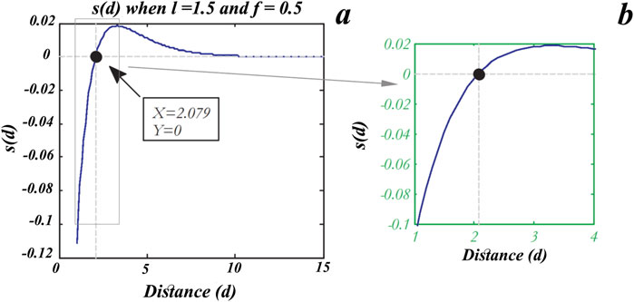
Figure 3. Compacting the repulsion and attraction between grasshoppers as social interactions in the ranges of (A) [0, 15] and (B) [1, 4].

Figure 4

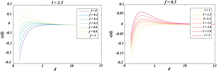
Figure 4. Effects of varying the values of parameters l and f on the function s(d).

Figure 5

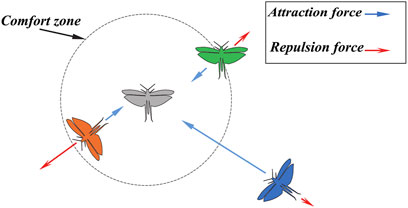
Figure 5. Conceptual plan of the comfort zone employing the function s and interactions between grasshoppers.

This model cannot be optimized because it is meant for swarms in free space, and its application avoids the exploration and exploitation procedures around a solution in the desired space (Saremi et al., 2017). Therefore, a modified version of Equation 14 is presented as follows:

$Y_i^d=c\left({\displaystyle \sum _{j=1}^N}c\frac{{ub}_d-{lb}_d}{2}s\left(\left|x_j^d-x_i^d\right|\right)\frac{x_j-x_i}{d_{ij}}\right)+{\widehat{\mathrm{C}}}_d,(15)$

where c is the optimizer coefficient related to the modified attraction zone (promising exploitation region), repulsion zone (exploration of the search space), and comfort zone (balance between exploration and exploitation). Here, lb_d and ub_d are the lower and upper bounds of s(r), respectively, and ${Ĉ}_d$ is the value of the target. Figure 6 shows an example of the swarm behavior based on Equation 15. Here, s is calculated similarly based on the factor S in Equation 10. Moreover, the components W_i and P_i are always considered toward a target (${Ĉ}_d$) in this work. The grasshoppers should achieve balance between the exploration and exploitation procedures to reach the optimal comfort zone such that the GOA does not fall into a local minimum and provides an accurate estimation of the global optimum point. Factor c is the most significant director parameter of the GOA and is updated as follows:

$c=c_{\mathit{max}}-l\frac{c_{\mathit{max}}-c_{\mathit{min}},}{L}(16)$

where c_min = 0.00004, c_max = 1, and L and l are the total number of iterations and current iteration, respectively.

Figure 6

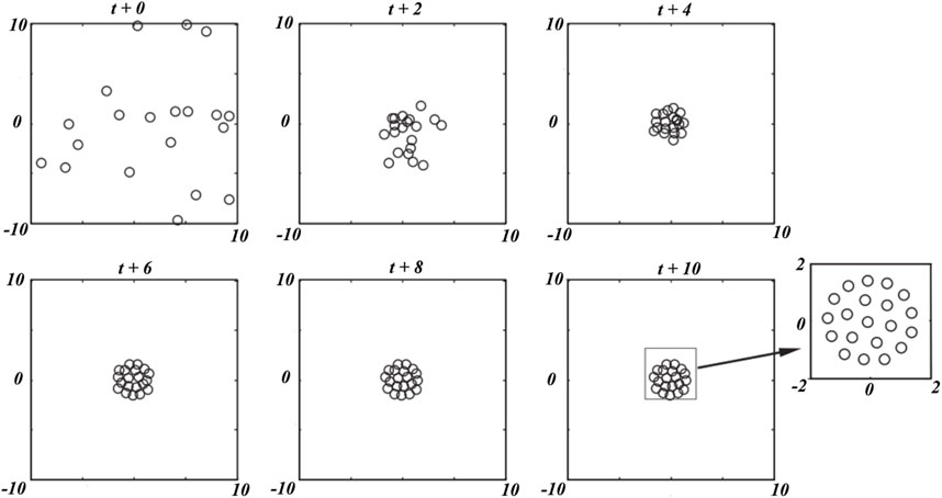
Figure 6. Example of grasshopper swarm behavior.

3.3 Fitted validation tool

3.3.1 Confusion matrix

The confusion matrix is an efficient tool that is frequently employed to estimate the prediction accuracy of a supervised ML algorithm (Bigdeli et al., 2022; Ge et al., 2022; Liu et al., 2005; Parsa et al., 2018). This matrix assesses the exact performance of the supervised classification model. For a two-class classifier with data labels 0 and 1 indicating the respective negative and positive solutions, the confusion matrix produces four consequences, namely, false negative (FN) that introduces a feature with class label 0 and incorrect classification, true negative (TN) that introduces a feature with class label 0 and correct classification, false positive (FP) that introduces a feature with class label 1 and incorrect classification, and true positive (TP) that introduces a feature with class label 1 and correct classification. Additionally, the confusion matrix presents the degrees of efficiency, precision, and accuracy of a supervised classifier. The parameters of the confusion matrix for a supervised model are calculated as follows:

$\text{Specificity}=\frac{TN}{TN+FP.}(17)$

$\text{Sensitivity}=\frac{TP}{TP+FN}.(18)$

$\text{Precision}=\frac{TP}{TP+FP}.(19)$

$\text{Negative\hspace{0.17em}\hspace{0.17em}predictive\hspace{0.17em}\hspace{0.17em}value\hspace{0.17em}\hspace{0.17em}}\left(\text{NPV}\right)=\frac{TN}{TN+FN.}(20)$

$\text{Accuracy}=\frac{TP+TN}{TP+FP+TN+FN}.(21)$

Thus, the confusion matrix was employed to compare the degree of efficiency of the grasshopper-optimized support vector machine (GSVM) with various kernel functions.

3.3.2 Receiver operating characteristic (ROC) curve

The ROC curve is employed as an aggregated classification method to validate the geochemical data. The area under the ROC curve (AUC) is measured to determine the reliability, influence, and numerical assessment of model performance or data classification. The AUC value mostly lies in the range of [0.5, 1]. When the AUC value is 0.5, the performance of the applied ML model or classified data is similar to a random guess. When the AUC is 1, the performance of the applied ML model is considered to be perfect; in other words, AUC = 1 means that the applied ML model has been trained perfectly or that the training data are categorized correctly.

4 Results and discussion

4.1 Preparing training data

A total of 800 stream sediment samples were collected to check the changes rates of the concentrations of 38 elements using the induced coupled plasma mass spectrometry (ICP-MS) technique with precision less than 10% (Sabbaghi, 2018). The isometric log-ratio (ilr) transformation was employed to remove the data closure problem as per Equation 22 (Sadeghi et al., 2024; Wang et al., 2014). Then, the geochemical data of the stream sediments were transformed into the range of [0, 1] to train the applied models.

$\text{ilr}\left(\mathrm{x}\right)=\sqrt{\frac{D-i}{D-i+1}}\left(\log \left(\frac{x_i}{g\left(x\right)}\right)\right)\left(i=1,2,\dots ,D-1\right),(22)$

where x, x_D, and g(x) indicate the vector of a composition with D dimensions, Euclidean distances between the distinct variables, and geometric mean of the composition x, respectively (Aitchison et al., 2000). Accordingly, a geochemical data table comprising the transformed values of elements Pb, Zn, Ag, and Cd was constructed to delineate the geochemical populations in the study area. Thus, the geochemical data table had four columns, including the transformed values of the pathfinder elements, with one column including the labels and 800 rows including the individual collected samples to train the model. To assign the predefined labels of the training data, we applied several ranges of transformed values (Table 1). Accordingly, the label 2 was assigned to geochemical samples with the criterion Pb + Zn + Ag + Cd ≥ 2.762 and label 1 was allocated to samples with the criterion 2.726 > Pb + Zn + Ag + Cd > 0. For example, a geochemical sample with the transformed values of Pb = 0.612, Zn = 0.751, Ag = 0.648, and Cd = 0.806 is a member of the geochemical anomaly population and has the label 2.

Table 1

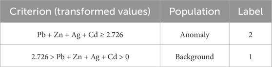
Table 1. Applied criteria for assigning the training data labels.

4.2 Training the GSVM model

The ability of the GOA to seek search spaces for discovering the optimal solutions of challenging problems is shown in Figure 6. Here, the GOA is fittingly attracted to optimal solutions in the best locations of the search spaces, and the number of random parameters is restricted in the GOA. Therefore, the initial population of grasshoppers is significant in this algorithm. The relevant hyperparameters, including kernel size (σ) of the RBF, kernel order (d) of the PF, and objective function parameter (penalty value C), are important such that differences in their values can produce various classification conclusions of the SVM model. Furthermore, trial-and-error procedures are time-consuming and onerous that may not always provide reliable results. Therefore, the hyperparameters of the RBF-SVM and PF-SVM models should be optimized using a metaheuristic optimization algorithm that is quick, easy, and also provides reliable results. The present study entails reliable optimization of the aforementioned hyperparameters using a known swarm-intelligence optimization algorithm that is not time-consuming. A schematic of the GSVM framework is presented in Figure 7; here, MATLAB R2022a was applied to the GSVM model. After preprocessing, the 800 collected samples were divided into the testing (30%) and training (70%) data in terms of the percentage of anomaly and background population. For model training, the required parameters are number of grasshoppers, maximum number of iterations, K-fold cross validation, lower bound, and upper bound, which were empirically set to 20, 100, 10, 0, and 10, respectively. The optimized values of the hyperparameters are presented in Table 2, and the results of the training data classification are shown in Figure 8. Accordingly, the precision and accuracy of training the GSVM with the RBF kernel are 90.48% and 98.21% (Figure 8A), while the results with the PF kernel are 92.86% and 98.75% (Figure 8B), respectively. Furthermore, the specificity and sensitivity of the trained GSVM are suitable. In fact, the specificity (99.22% and 99.42%) as well as sensitivity (86.36% and 90.7%) of the GSVM with the corresponding RBF (Figure 8A) and PF (Figure 8B) kernels prove that the GSVM model has been trained efficiently.

Figure 7

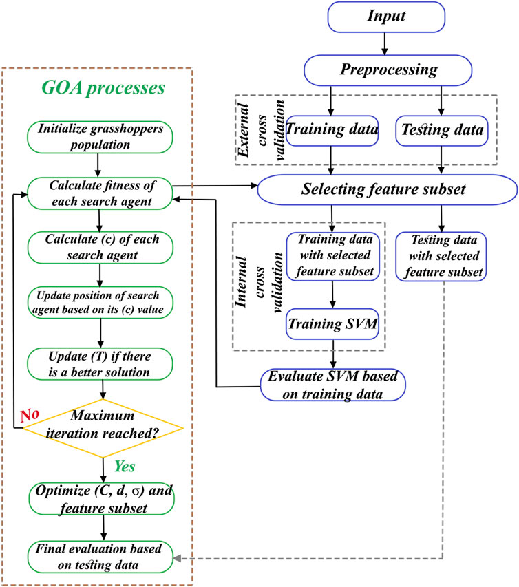
Figure 7. Schematic of the grasshopper-optimized support vector machine (GSVM) framework.

Table 2

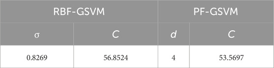
Table 2. Optimized values of the hyperparameters of the GSVM model for both kernels.

Figure 8

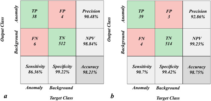
Figure 8. Confusion matrices for training the GSVM network with (A) radial basis function (RBF) and (B) polynomial function (PF) kernels.

In the present work, we also decreased the root mean-squared error (RMSE) associated with the cost function values, as shown in Equation 23, during training.

$RMSE=\sqrt{\frac{1}{n}\left({\displaystyle \sum _{i=1}^n}\left(C_R-C_p\right)\right),}(23)$

where n, C_R, and C_p are the number of geochemical samples, real class allocated to the sample, and predicted class of the sample, respectively. Figure 9 shows that the GSVM models with both kernels can achieve the most optimized states of classification. SVM optimization with the RBF kernel was implemented to 42 iterations, at which point the value converged to 0.088 (Figure 9A). Figure 9B depicts that SVM optimization with the PF kernel was implemented to 45 iterations and that the converged value is 0.052. Both cost functions (Figure 9) are noted to have been in their steady states for more than 40 iterations, thereby ensuring good model optimization. The effects of these procedures on the mapping of the geochemical testing data are shown in Figure 10. Figure 10A shows the multi-element geochemical map of the testing data classified using the RBF-GSVM, and Figure 10B shows the corresponding map when using the PF-GSVM. Although both kernels can detect multi-element geochemical anomalies with the GSVM model, the PF kernel (Figure 10B) obviously has more accuracy. Figure 11 exhibits the validation of the GSVM model with the testing data; it can be observed that the results of the GSVM model for both kernels have precision of 100% and impressive accuracies (98.33% and 99.17%), making them the ideal choice for classifying the testing data. Here, the sensitivity of the RBF-GSVM is lower than that of the PF-GSVM because the number of predicted FN values has increased. The GSVM with RBF kernel labels more background samples as anomalies than the GSVM with PF kernel. The ROCs presented in Figure 12 show the comparison of the prediction abilities of the trained models in this work. The PF-GSVM has greater accuracy than that of the RBF-GSVM model as the AUC values of the testing data classification (class 2 = 0.973, class 1 = 0.961) with the PF-SVM (Figure 12B) are greater than the AUC values (class 2 = 0.969, class 1 = 0.957) obtained with the RBF-SVM (Figure 12A).

Figure 9

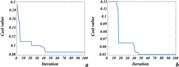
Figure 9. Cost function values for optimizing the GSVM model with (A) RBF and (B) PF kernels.

Figure 10

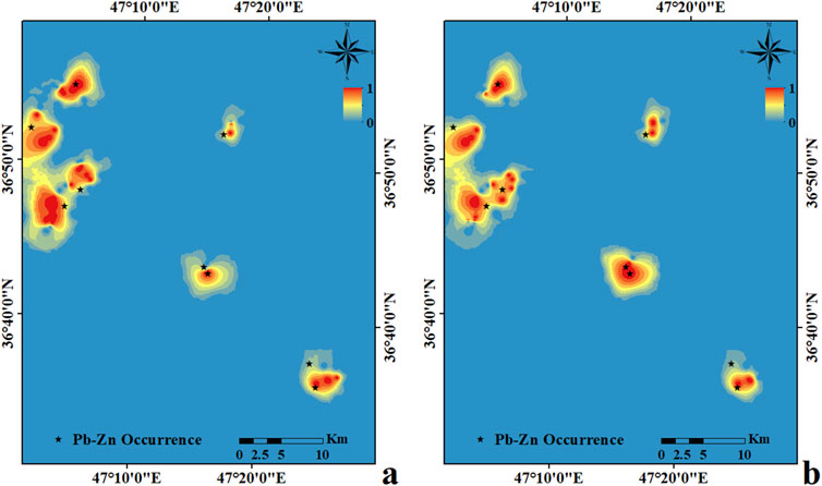
Figure 10. Multi-element geochemical maps (Pb–Zn–Ag–Cd) plotted using the GSVM algorithm with (A) RBF and (B) PF kernels.

Figure 11

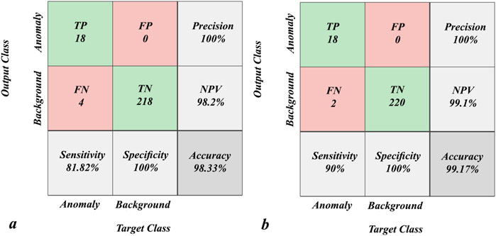
Figure 11. Confusion matrices for testing the GSVM network with (A) RBF and (B) PF kernels.

Figure 12

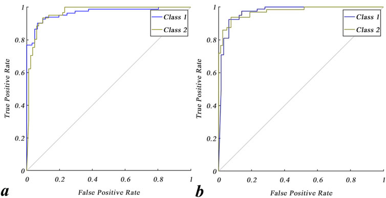
Figure 12. Receiver operating characteristic (ROC) curves for testing the GSVM network with (A) RBF and (B) PF kernels.

5 Conclusion

The present study involves successful optimization of the effective hyperparameters of the PF-SVM and RBF-SVM, which are popular and practical modeling approaches in various geoscientific fields. The objective of this work was to propose an SVM for classification of multi-element geochemical data that is not limited by trial-and-error values of the hyperparameters because applying the SVM with its non-linear functions requires optimization of the relevant hyperparameters. Fortunately, the GOA was found to reliably optimize the hyperparameters of the PF-SVM and RBF-SVM in the shortest possible time without trial-and-error procedures. The proposed model was successfully employed to recognize multi-element geochemical anomalies related to Pb–Zn mineralizations in the Takht-e Soleyman area of northwest Iran. Confusion matrices of the training data show that the GSVM model has been trained appropriately and can classify results accurately for the testing data. Multi-element geochemical maps of the testing data classification show that the GSVM with PF kernel has more accuracy than the GSVM with RBF kernel. Furthermore, reduced and constant cost function values of 0.08 and 0.05 were obtained following optimization, which proves that the PF-SVM and RBF-SVM models can be reliably optimized without excess time consumption. The present work can be extended to the optimization of the hyperparameters of other known ML models with various metaheuristic algorithms in future studies.

Data availability statement

The original contributions presented in this study are included in the article/supplementary material, and any further inquiries may be directed to the corresponding author.

Ethics statement

Ethical approval was not required for the study involving humans in accordance with the local legislation and institutional requirements. Written informed consent to participate in this study was not required from the participants or their legal guardians/next of kin in accordance with the national legislation and institutional requirements. Written informed consent was obtained from individuals and minors’ legal guardians/next of kin for the publication of any potentially identifiable images or data included in this article.

Author contributions

HS: conceptualization, formal analysis, investigation, methodology, software, validation, visualization, and writing–original draft. ST: data curation, formal analysis, supervision, and writing–original draft. NF: supervision, writing–review and editing.

Funding

The authors declare that no financial support was received for the research, authorship, and/or publication of this article.

Acknowledgments

The authors wish to thank the geological survey & mineral exploration organization of Iran for the geochemical data collected for this study.

Conflict of interest

The authors declare that the research was conducted in the absence of any commercial or financial relationships that could be construed as a potential conflict of interest.

Publisher’s note

All claims expressed in this article are solely those of the authors and do not necessarily represent those of their affiliated organizations, or those of the publisher, the editors and the reviewers. Any product that may be evaluated in this article, or claim that may be made by its manufacturer, is not guaranteed or endorsed by the publisher.

References

Abedi, M., Norouzi, G.-H., and Bahroudi, A. (2012). Support vector machine for multi-classification of mineral prospectivity areas. Comput. Geosciences 46, 272–283. doi:10.1016/j.cageo.2011.12.014

CrossRef Full Text | Google Scholar

Aitchison, J., Barceló-Vidal, C., Martín-Fernández, J. A., and Pawlowsky-Glahn, V. (2000). Logratio analysis and compositional distance. Math. Geol. 32, 271–275. doi:10.1023/a:1007529726302

CrossRef Full Text | Google Scholar

Anderson, J. A. (1972). A simple neural network generating an interactive memory. Math. Biosci. 14, 197–220. doi:10.1016/0025-5564(72)90075-2

CrossRef Full Text | Google Scholar

Bigdeli, A., Maghsoudi, A., and Ghezelbash, R. (2022). Application of self-organizing map (SOM) and K-means clustering algorithms for portraying geochemical anomaly patterns in Moalleman district, NE Iran. J. Geochem. Explor. 233, 106923. doi:10.1016/j.gexplo.2021.106923

CrossRef Full Text | Google Scholar

Carranza, E. J. M. (2008). Geochemical anomaly and mineral prospectivity mapping in GIS. Elsevier.

Google Scholar

Cheng, Q., Xu, Y., and Grunsky, E. (2000). Integrated spatial and spectrum method for geochemical anomaly separation. Nat. Resour. Res. 9, 43–52. doi:10.1023/a:1010109829861

CrossRef Full Text | Google Scholar

Coates, A., Ng, A., and Lee, H. (2011). “An analysis of single-layer networks in unsupervised feature learning,” in Proceedings of the fourteenth international conference on artificial intelligence and statistics, 215–223.

Google Scholar

Cox, D. R. (1958). The regression analysis of binary sequences. J. R. Stat. Soc. Ser. B Methodol. 20, 215–232. doi:10.1111/j.2517-6161.1958.tb00292.x

CrossRef Full Text | Google Scholar

Dietterich, T. (2002). “Ensemble learning,” in The handbook of brain theory and neural networks. Editor M. A. Arbib 2nd Edn, 110–125.

Google Scholar

Ge, Y.-Z., Zhang, Z.-J., Cheng, Q.-M., and Wu, G.-P. (2022). Geological mapping of basalt using stream sediment geochemical data: case study of covered areas in Jining, Inner Mongolia, China. J. Geochem. Explor. 232, 106888. doi:10.1016/j.gexplo.2021.106888

CrossRef Full Text | Google Scholar

Geranian, H., Tabatabaei, S. H., Asadi, H. H., and Carranza, E. J. M. (2016). Application of discriminant analysis and support vector machine in mapping gold potential areas for further drilling in the Sari-Gunay gold deposit, NW Iran. Nat. Resour. Res. 25, 145–159. doi:10.1007/s11053-015-9271-2

CrossRef Full Text | Google Scholar

Ghezelbash, R., Maghsoudi, A., and Carranza, E. J. M. (2020). Optimization of geochemical anomaly detection using a novel genetic K-means clustering (GKMC) algorithm. Comput. Geosci. 134, 104335. doi:10.1016/j.cageo.2019.104335

CrossRef Full Text | Google Scholar

Gonbadi, A. M., Tabatabaei, S. H., and Carranza, E. J. M. (2015). Supervised geochemical anomaly detection by pattern recognition. J. Geochem. Explor. 157, 81–91. doi:10.1016/j.gexplo.2015.06.001

CrossRef Full Text | Google Scholar

Hinton, G. E., Osindero, S., and Teh, Y.-W. (2006). A fast learning algorithm for deep belief nets. Neural Comput. 18, 1527–1554. doi:10.1162/neco.2006.18.7.1527

PubMed Abstract | CrossRef Full Text | Google Scholar

Hosseini-Dinani, H., and Aftabi, A. (2016). Vertical lithogeochemical halos and zoning vectors at Goushfil Zn–Pb deposit, Irankuh district, southwestern Isfahan, Iran: implications for concealed ore exploration and genetic models. Ore Geol. Rev. 72, 1004–1021. doi:10.1016/j.oregeorev.2015.09.023

CrossRef Full Text | Google Scholar

LeCun, Y., Bengio, Y., and Hinton, G. (2015). Deep learning. Nature 521 (7553), 436–444. doi:10.1038/nature14539

PubMed Abstract | CrossRef Full Text | Google Scholar

Liu, C., Berry, P. M., Dawson, T. P., and Pearson, R. G. (2005). Selecting thresholds of occurrence in the prediction of species distributions. Ecography 28, 385–393. doi:10.1111/j.0906-7590.2005.03957.x

CrossRef Full Text | Google Scholar

Maepa, F., Smith, R. S., and Tessema, A. (2021). Support vector machine and artificial neural network modelling of orogenic gold prospectivity mapping in the Swayze greenstone belt, Ontario, Canada. Ore Geol. Rev. 130, 103968. doi:10.1016/j.oregeorev.2020.103968

CrossRef Full Text | Google Scholar

Parsa, M., Maghsoudi, A., and Yousefi, M. (2018). A receiver operating characteristics-based geochemical data fusion technique for targeting undiscovered mineral deposits. Nat. Resour. Res. 27, 15–28. doi:10.1007/s11053-017-9351-6

CrossRef Full Text | Google Scholar

Redlich, A. N. (1993). Redundancy reduction as a strategy for unsupervised learning. Neural Comput. 5, 289–304. doi:10.1162/neco.1993.5.2.289

CrossRef Full Text | Google Scholar

Sabbaghi, H. (2018). A combinative technique to recognise and discriminate turquoise stone. Vib. Spectrosc. 99, 93–99. doi:10.1016/j.vibspec.2018.09.002

CrossRef Full Text | Google Scholar

Sabbaghi, H., and Moradzadeh, A. (2018). ASTER spectral analysis for host rock associated with porphyry copper-molybdenum mineralization. J. Geol. Soc. India 91, 627–638. doi:10.1007/s12594-018-0914-x

CrossRef Full Text | Google Scholar

Sabbaghi, H., and Tabatabaei, S. H. (2020). A combinative knowledge-driven integration method for integrating geophysical layers with geological and geochemical datasets. J. Appl. Geophys. 172, 103915. doi:10.1016/j.jappgeo.2019.103915

CrossRef Full Text | Google Scholar

Sabbaghi, H., and Tabatabaei, S. H. (2022). Application of the most competent knowledge-driven integration method for deposit-scale studies. Arabian J. Geosciences 15, 1057–1110. doi:10.1007/s12517-022-10217-z

CrossRef Full Text | Google Scholar

Sabbaghi, H., and Tabatabaei, S. H. (2023a). Data-driven logistic function for weighting of geophysical evidence layers in mineral prospectivity mapping. J. Appl. Geophys. 212, 104986. doi:10.1016/j.jappgeo.2023.104986

CrossRef Full Text | Google Scholar

Sabbaghi, H., and Tabatabaei, S. H. (2023b). Execution of an applicable hybrid integration procedure for mineral prospectivity mapping. Arabian J. Geosciences 16, 3–13. doi:10.1007/s12517-022-11094-2

CrossRef Full Text | Google Scholar

Sabbaghi, H., and Tabatabaei, S. H. (2023c). Regimentation of geochemical indicator elements employing convolutional deep learning algorithm. Front. Environ. Sci. 11, 1076302. doi:10.3389/fenvs.2023.1076302

CrossRef Full Text | Google Scholar

Sabbaghi, H., Tabatabaei, S. H., and Fathianpour, N. (2024). Geologically-constrained GANomaly network for mineral prospectivity mapping through frequency domain training data. Sci. Rep. 14, 6236. doi:10.1038/s41598-024-56644-8

PubMed Abstract | CrossRef Full Text | Google Scholar

Sadeghi, B., Molayemat, H., and Pawlowsky-Glahn, V. (2024). How to choose a proper representation of compositional data for mineral exploration? J. Geochem. Explor. 259, 107425. doi:10.1016/j.gexplo.2024.107425

CrossRef Full Text | Google Scholar

Saremi, S., Mirjalili, S., and Lewis, A. (2017). Grasshopper optimisation algorithm: theory and application. Adv. Eng. Softw. 105, 30–47. doi:10.1016/j.advengsoft.2017.01.004

CrossRef Full Text | Google Scholar

Scott, A. J., and Knott, M. (1974). A cluster analysis method for grouping means in the analysis of variance. Biometrics 30, 507–512. doi:10.2307/2529204

CrossRef Full Text | Google Scholar

Vapnik, V. (1999). The nature of statistical learning theory. Springer Science and Business Media.

Google Scholar

Wang, W., Zhao, J., and Cheng, Q. (2014). Mapping of Fe mineralization-associated geochemical signatures using logratio transformed stream sediment geochemical data in eastern Tianshan, China. J. Geochem. Explor. 141, 6–14. doi:10.1016/j.gexplo.2013.11.008

CrossRef Full Text | Google Scholar

Wei, H., Xiao, K., Shao, Y., Kong, H., Zhang, S., Wang, K., et al. (2020). Modeling-based mineral system approach to prospectivity mapping of stratabound hydrothermal deposits: a case study of MVT Pb-Zn deposits in the Huayuan area, northwestern Hunan province, China. Ore Geol. Rev. 120, 103368. doi:10.1016/j.oregeorev.2020.103368

CrossRef Full Text | Google Scholar

Zuo, R., and Carranza, E. J. M. (2011). Support vector machine: a tool for mapping mineral prospectivity. Comput. Geosci. 37, 1967–1975. doi:10.1016/j.cageo.2010.09.014

CrossRef Full Text | Google Scholar