Modeling snow optical properties from single wavelength airborne lidar in steep forested terrain

Airborne lidar is a powerful tool used by water resource managers to map snow depth and aid in producing spatially distributed snow water equivalent (SWE) when combined with modeled density. However, limited research so far has focused on retrieving optical snow properties from lidar. Optical snow surface properties directly impact albedo, which has a major control on snowmelt timing, which is especially useful for water management applications. Airborne lidar instruments typically emit energy at a wavelength of 1,064 nm, which can be informative in mapping optical snow surface properties since grain size modulates reflectance at this wavelength. In this paper we present and validate an approach using airborne lidar for estimating snow reflectance and optical grain size at high spatial resolution. We utilize three lidar flights over the Boise National Forest, United States, during a winter season from December 2022 to March 2023. We discuss sensitivities to beam incidence angles, compare results to in situ measurements snow grain size, and perform spatial analyses to ensure reflectance and optical grain size varies across space and time as anticipated. Modeled optical grain size from lidar performed well (Root mean squared difference = 49 μm; percent mean absolute difference = 31%; n = 28), suggesting that aerial lidar surveys can be useful in mapping snow reflectance and optical grain size for dry snow, and may support development of other remote sensing technologies and aid water resources management.

1 Introduction

Snow albedo is a crucial variable in snow remote sensing and water resource management because of the magnitude of incoming solar radiation reflected (Warren, 1982). Since snow covers 12%–33% of the global land mass, snow albedo is a major control on global energy balance. However, snow grains at the surface undergo constant change across the landscape from the time snow falls until it melts (Colbeck, 1982). In the absence of light absorbing particles (e.g., soot, dust, algae) and liquid water, the visible near-infrared (VNIR) reflectance of snow is almost entirely controlled by optical grain size (Warren, 1982), and to a smaller extent by grain shape (He et al., 2017). Determining optical grain size is a benefit to water resource management decisions, as it influences the energy balance of snow and consequent grain metamorphism, which changes albedo and therefore melt (Painter et al., 2016). Tracking global snow metamorphism and its impact on albedo will improve estimation of snowmelt timing, which has large scale financial and societal implications for communities and ecosystems (Sturm et al., 2017). Monitoring global snowpack reservoirs is important, as about one-sixth of the world’s population relies on snowmelt (Barnett et al., 2005).

Better methods for mapping optical grain size are valuable and required for improving energy balance modeling (He et al., 2017; Räisänen et al., 2017), through model development, as well as uncertainty quantification in data assimilation (Durand and Margulis, 2008). There are many existing datasets for this purpose. For example, Moderate Resolution Imaging Spectroradiometer (MODIS) can be processed with algorithms such as Snow Property Inversion From Remote Sensing (SPIReS) (Bair et al., 2020) and MODIS Snow Covered Area and Grain-size (MODSCAG) (Painter et al., 2009) to estimate snow properties. Additionally, there has been extensive research to create highly accurate optical grain size maps from hyperspectral AVIRIS flights (Nolin and Dozier, 1993; Nolin and Dozier, 2000) and assess the uncertainty of these quantifications (Painter et al., 2013). The high solar zenith angles–a fact of winter in the sub-arctic and cryosphere–are a large limitation for grain size retrieval methods relying on passive sensors (Bohn et al., 2021; Fair et al., 2022; Yang et al., 2017).

Topography provides an additional challenge in collecting signals with already high solar zenith angles–further changing the local surface incidence angle and creating possible sources for error (Dozier et al., 2022). Precise characterization of the optical path (incoming and outgoing) is therefore important. High resolution lidar measuring both structural and optical information can meet these challenges in complex topography and less than ideal illumination conditions, allowing us to attempt to solve optical grain size from the received lidar signal.

Previous work has established a proof of concept for estimating optical grain size using spaceborne lidar with pulse wavelength at 1,064 nm (Yang et al., 2017), since reflectance of snow is highly sensitive to changes at this wavelength (Warren, 1982). Yang et al. (2017) modeled optical grain size using analytical asymptotic radiative transfer theory (AART) (Kokhanovsky and Zege, 2004) over polar icesheets with ICESAT GLAS as input, finding general patterns of optical grain size distributions consistent with past research for these regions (Gay et al., 2002). Ackroyd et al. (2024) demonstrated promising results using this same method for both airborne and Unmanned Aerial System (UAS) platforms. In their study, they found reliable optical grain size estimates (mean absolute error = 32 $\mu$ m) when compared to in situ field observations in Colorado, United States.

However, limited attention has been given to rigorously testing uncertainty of optical grain size using airborne lidar. This is especially important considering current spaceborne instruments such as Environmental Mapping and Analysis Program (EnMAP), Hyperspectral Precursor of the Application Mission (PRISMA), and Earth Surface Mineral Dust Source Investigation (EMIT), as well as upcoming missions such as NASA Surface Biology and Geology (SBG) and ESA Copernicus Hyperspectral Imager Mission for Environment (CHIME), which will be able to leverage global imaging spectroscopy data to model snow properties at the surface, like optical grain size and snow albedo (Cawse-Nicholson et al., 2021; Cogliati et al., 2021; Kokhanovsky et al., 2023; Thompson et al., 2024). However, solving uncertainties for high incidence angle observations is needed to improve model performance (Bohn et al., 2021). Airborne lidar derived optical grain sizes are independent of sun illumination, therefore, if uncertainty metrics are well known for lidar it could be a valuable in informing such satellite missions. Also, lidar can penetrate canopy, which remains a limitation for multispectral and hyperspectral remote sensing (Dozier and Painter, 2004; Kane et al., 2008; Liu et al., 2004; Muhuri et al., 2021; Nolin, 2010; Raleigh et al., 2013; Vikhamar and Solberg, 2003). Accurately mapping snow properties in forest ecosystems remains crucially important for our ability to monitor and understand ecohydrological processes as snowmelt timing shifts in a warming climate (Harpold, 2016). In North America alone, forests make up approximately 40% of the snow-covered area (Klein et al., 1998).

To these ends, we build upon past studies (Ackroyd et al., 2024; Yang et al., 2017) and leverage helicopter-flown airborne lidar over the Boise National Forest in Idaho, United States, to estimate optical grain size and perform uncertainty testing in areas of forest cover and high incidence angles. We address the following key questions to develop the efficacy of this technique:

• At what incidence angle does retrieved reflectance from airborne lidar over snowy terrain become unreliable using an incidence angle correction method?

• Can airborne lidar be used to estimate snow reflectance and optical grain size accurately in steep, forested terrain? And in doing so, what are the associated uncertainties?

• How does lidar derived optical grain size vary throughout the season and across a landscape, and do these distributions match what we would expect given past research and observations?

2 Methods

2.1 Study site

We analyzed helicopter-mounted lidar (Riegl VQ 580 ii; O’Neel et al., 2022) over the Boise National Forest in Southwest Idaho, United States (Figure 1). Three flights were analyzed including 8 December 2022, 9 February 2023, and 16 March 2023. The 35 km² study site is covered predominately with conifers such as lodgepole pine (Pinus contorta), ponderosa pine (Pinus ponderosa), and Douglas-fir (Pseudotsuga menziesii). In 2016, the Pioneer Fire burned approximately 767 km² of the Boise National Forest, and approximately half of our study area. We assumed light absorbing particles at the surface to be minimal given the study was conducted 7 years after the fire and during the accumulation season (Gleason et al., 2019; Uecker et al., 2020). With this assumption, and the fact that these constituents have a small impact on the 1,064 nm wavelength (Miller et al., 2016), we did not account for light absorbing particles in our study. We also assumed no dust was present at our site; however, episodic dust events can be common in the western United States and can impact the VNIR reflectance depending on the dust radius (Warren and Wiscombe, 1980).

Figure 1

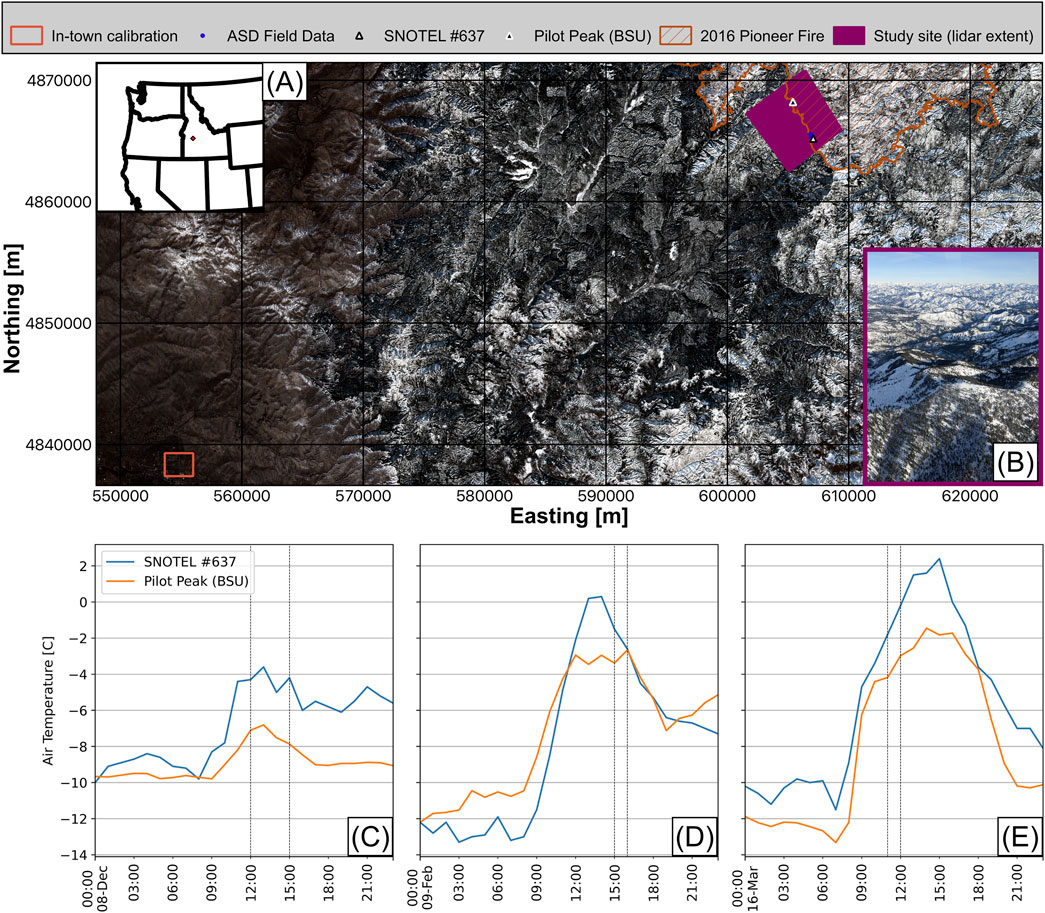
Figure 1. Study site in southern Idaho shown in WGS84 UTM 11 N (EPSG: 32611) with Sentinel-2 true color from February composite as the basemap (A), and portion of study site shown from the helicopter on 9 February 2023 (B). Hourly air temperature was recorded across the site for December flight (C), February flight (D), and March flight (E). Dashed lines represent window of flight time. Air temperatures were below freezing during flights suggesting minimal liquid water content at surface.

The elevation range of our study area is 1,563 to 2,463 m above mean sea level. The mean precipitation for this site ranges widely based on elevation and interannual variability, but typically received about 1,150 mm according to the last 10 years of data at Mores Creek SNOTEL #637. Snow depth was optically thick for all flights. Each flight included a boresight calibration in a residential area in Eagle, Idaho (60 km away from the study site) which is highlighted as in-town calibration in Figure 1.

2.2 Snow conditions and collection of field data

Estimating optical grain size from single wavelength airborne lidar relies on the assumption of dry snow. This is because the presence of liquid water will shift the ice absorption window, therefore, requiring more than one wavelength to resolve grain size and water content (Donahue et al., 2022). Observed air temperatures were below 0°C during the duration of all three flights for both a station at Pilot Peak (elevation = 2,450 m) and at the nearby SNOTEL station (elevation = 1,859 m), indicating minimal liquid water at the surface during data collection (Figures 1C–E).

Low-lying clouds were present between the ground surface and the lidar system mounted on the helicopter for some of the flightlines of the 8 December 2022 flight, reducing the returned intensity (Supplementary Figure S1). We discarded these flightlines and retained 10 cloud-free flightlines for this date for our spectral observations; all flightlines were used to create a high-resolution terrain product for this date.

We collected a transect of in situ field spectroscopy for the December and February flights, over a 1-h window during solar noon. Locations of measurements were recorded at each point using an Emlid Reach RS2 attached to a plumb 3 m survey pole to ensure the ground (below snow) was reached. We collected diffuse incoming solar irradiance, total incoming irradiance, and upwelling diffuse radiance using an ASD FieldSpec 4 (calibrated Summer 2022) with the remote cosine receptor on the end of a 1 m aluminum rod-held plumb held roughly waist high. We recorded the diffuse component using a small cardboard disk on a pole to shade the receptor (Supplementary Figure S2). We chose this method instead of an 8-degree field of view fore-optic (Skiles et al., 2023), because our points were in steep terrain (slopes to 21°), although solving for grain size using hemispherical measurements is a difficult problem in complex terrain. Alternative methods using instruments that are terrain independent may be better suited for measuring optical grain size, such as contact spectroscopy (Painter et al., 2007), integrating sphere (Gallet et al., 2009), IRIS (Montpetit et al., 2012), or IceCube (Zuanon, 2013). Future studies that seek to validate grain size in sloped terrain may be interested in using terrain independent methods.

2.3 Correcting ground data for sloped terrain

Raw hemispherical data were collected and were converted to intrinsic spectral albedo (${\alpha }_{\lambda }^i$) by accounting for the local solar zenith angle due to the terrain (Bair et al., 2018) using following Equation 1,

${\alpha }_{\lambda }^i=\frac{F_{\lambda ,dif}^{\uparrow }}{F_{\lambda ,dif}^{\downarrow }+{cF}_{\lambda ,dir}^{\downarrow }}(1)$

where $F_{\lambda ,dif}^{\uparrow }$ is the upwelling diffuse radiation measured by pointing the sensor down, $F_{\lambda ,dir}^{\downarrow }$ is the downwelling direct irradiance measured by pointing the sensor up, and $F_{\lambda ,dif}^{\downarrow }$ is the downwelling diffuse irradiance measured in the same location as the direct irradiance measurement, but occluded (shaded) from direct sun. Parameter c is the cosine of the local solar illumination angle (${\mu }_s$) divided by the cosine of the solar zenith angle of a flat surface (${\mu }_0$). For this parameter we used the slope and aspect products derived from coincident airborne lidar. The directional precision of the measurements (up or down) was ensured via bubble level attached to the aluminum rod.

Next, we used ${\alpha }_{\lambda }^i$ to estimate our ground truth optical grain size. To do this, we minimized the root mean squared difference (RMSD) between AART-derived plane albedo (Kokhanovsky et al., 2021) between 1,100–1,300 nm, allowing optical grain size to vary in a sequential least squares programming numerical optimization method (Kraft, 1988). The AART radiative transfer model was selected due to its simplicity and bi-directional reflectance distribution function (BRDF) product. Therefore, we were able to use the same model for both the inversion of snow properties from spectroscopy, as well as from lidar (discussed in Section 2.4), limiting any discrepancies in model assumptions. The range of 1,100–1,300 nm observed from spectroscopy was selected for our inversion window because it captures the strong variation in reflectance that is largely a function of optical grain size and also contains a relatively smaller amount of diffuse light from passive radiation. We also solved for each condition with ${\mu }_s$ +/− 0.01 to get at an estimate of measurement uncertainty using this retrieval method.

2.4 Estimating optical grain size from lidar data

To retrieve optical grain size from the returned laser pulse, we first needed to estimate the surface reflectance. Riegl (Horn, Austria) software supplied a reflectance product which was a function of the amplitude, range, and a white reference (Riegl, 2017), returned in raw dB (${\rho }_{raw}$). However, more processing is needed to account for factors that influence the attenuation of the lidar pulse (Wu et al., 2021). We estimated a calibrated reflectance ($\rho$) that accounts for local incidence angle, radiometric bias, and atmospheric transmittance using following Equation 2:

$\rho =\frac{{10}^{\frac{{\rho }_{raw}}{10}}}{\mu }\frac{C}{{\tau }^2}(2)$

where ${\rho }_{raw}$ is the relative reflectance output from Riegl in dB, $\tau$ is the atmospheric transmittance, $\mu$ is the cosine of the incidence angle of the lidar pulse and the surface normal, and C is the radiometric correction factor. Computation of each parameter and their required independent variables are described in the following subsections. Figure 2 shows a conceptual model refereced with subsection.

Figure 2

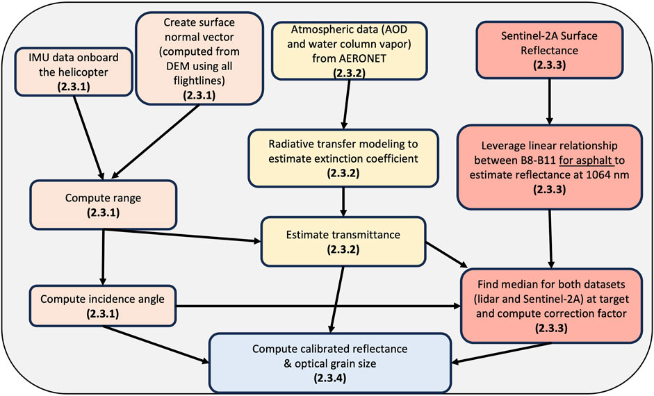
Figure 2. Overview of airborne lidar data collection and processing to output calibrated reflectance and optical grain size. Numbers shown in bold correspond to respective sub-section in the methods of this manuscript. Note we used all flightlines for a given date to create DSM and resulting surface normal.

2.4.1 Estimating the cosine of the local incidence angle ($\mathit{\mu }$)

To estimate $\mu$ we first estimated Range (R) by computing $\sqrt{X^2+Y^2+Z^2}$, where X, Y, and Z are the vectors from surface position to helicopter position. Onboard INSS IMU data were collected every 0.005 s with accuracy on the order of several cm. Based on our flight information (ground speed) and the speed of light for the lidar pulse, this temporal mismatch is estimated to contributed <0.1% errors in estimated μ which we consider a negligible influence for our analysis. To match helicopter position data with lidar pulses occurring at a higher frequency than the IMU, we used the closest matching internal GPS time using a rolling average function (“data.table”; Dowle et al., 2019). Surface normals were computed based on the resulting snow-on DSM at 0.5 m from all the flightlines merged (Beyer et al., 2018; Hoppinen et al., 2023; PDAL Contributors, 2022). We used bilinear interpolation to further smooth out the snow-on DSM to 3 m spatial resolution for our analysis in this paper. Surface normal vector < $n_i$, $n_j$, $n_k$ > were then computed using the following Equations 3–5:

$n_i=\sin \left(aspect\right)\sin \left(slope\right)(3)$

$n_j=\cos \left(aspect\right)\sin \left(slope\right)(4)$

$n_k=\cos \left(slope\right)(5)$

where $n_i$, $n_j$, and $n_k$ correspond to the x,y, and z components, respectively. For each flightline, we extracted the gridded surface normal at 3 m resolution, as well as snow depth and canopy height using the lidR package (“lidR”; Roussel et al., 2020; Roussel and Auty, 2023; Roussel and De Boissieu, 2023). Snow depth data were obtained by differencing the coincident lidar data with the reference snow-free DEM (Adebisi et al., 2022). Snow depth data were used to filter out non-snow points where snow depth was less than 0.08 cm (Stillinger et al., 2023) and canopy height was greater than 0 m. Then, we computed μ using Equation 6.

$\mu =\frac{X·n_i+Y·n_j+Z·n_k}{R·\sqrt{{n_i}^2+{n_j}^2+{n_k}^2}}(6)$

Following previous research, we removed lidar returns where $\mu$ < 0.5 (i.e., incidence angles greater than 60°) due to the overcorrection effect of $\mu$ in (3) at higher incidence angles (Ackroyd et al., 2024; Yan and Shaker, 2017). To test where overcorrection effect occurred for airborne lidar collection over snow we randomly selected a flightline from each of the three dates. We computed the corrected reflectance and saved the corresponding $\mu$ to tables. We grouped by $\mu$ to the nearest thousandth place, and then used the mean values of each class to estimate the constrained, piece-wise linear function that best fit the data (‘mcp’; Lindeløv 2020). We constrained the “good data region” by strictly enforcing the slope to be zero (i.e., the region where reflectance is no longer a function of $\mu$). This breakpoint analysis was carried out for each of the 3 flight dates and provided a range of potential limits of μ. Note, that while this sensitivity study was undertaken, we ultimately were more conservative in our data products presented in this study by removing all data where $\mu$ < 0.5 (Ackroyd et al., 2024).

2.4.2 Estimating the transmittance ($\mathit{\tau }$)

$\tau$ is a function of extinction coefficient ($a$) and range (or path length) (R) based on the Beer-Lambert Law (Swinehart, 1962),

$\tau =e^{-aR}(7)$

The extinction coefficient is dependent on the atmospheric conditions during flight which is not known. However, we used the AERONET station in Meridian, Idaho at altitude 0.808 km for daily average water column vapor and aerosol optical depth (AOD) at 870 nm (Table 1). The Meridian AERONET site was roughly 10 km away from the Eagle, Idaho, calibration site and roughly 75 km from the study site. We assume that water column vapor and AOD at 870 nm were similar for the AERONET site, boresight location, and study site for a given date. Assuming mid-latitude winter atmosphere, we estimated τ for 12 altitudes ranging from 0–3 km above sea level using libRadtran radiative transfer software, with DISORT pseudo-spherical approximation and number of streams equal to 16 (Mayer and Kylling, 2005). We then took the natural log of both sides of (8) to create a linear relationship between $\tau$ and changing altitude. The slope of this line is our approximation of $a$, which, for example, on the 9 February 2023 flight gave us $a$ = 0.0064 km-1 (R² = 0.99). This correlation is high because it is a function of elevation, and we limit the elevation range strictly to values of R we would expect to encounter during flight (e.g., 0–3 km). $\tau$ was then calculated for each lidar return dependent on R (Equation 7).

Table 1

Table 1. Atmospheric parameters from AERONET station “Meridian_DEQ” input into libRadtran for each of the flights. These values represent the average reported value for each lidar flight date. Resulting $a$ (extinction coefficient) is shown as well for each flight.

2.4.3 Estimating radiometric calibration factor (C)

A target with a known reflectance at 1,064 nm can be used to radiometrically correct lidar reflectance. However, this is not always feasible and there are many practical limitations to this method. Instead, we used a flat, asphalt target and assumed a strong linear relation between Bands 8 (centered ∼834 nm) and Band 11 (centered ∼1,614 nm) of Sentinel-2A based on prior in situ field spectroscopy measurements for a wide range of asphalt surfaces (Herold, 2004; Herold et al., 2008; Herold et al., 2008; R² = 0.99; Figure 3).

Figure 3

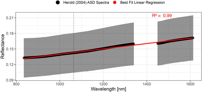
Figure 3. Average ASD spectra samples of asphalt (n = 46) shown in black with standard deviation bars collected in Herold (2004). The red line highlights the linear relationship (R² = 0.99) between wavelength and reflectance between 834 and 1,614 nm for asphalt. The wavelength at 1,064 nm is shown as a dotted black line for reference. Data from this spectral library were not used in analysis and are shown only for reference.

We used Sentinel-2A surface reflectance Bands 8 and 11 data from the closest match for each flight (less than 1 day a part for all flights). Using this interpolation method, we estimated the Sentinel-2A reflectance at 1,064 nm. The resulting Sentinel-2A reflectance was lower than the uncorrected lidar reflectance (example in Figure 4, February flight). Therefore, our correction factor (C) was found by dividing the median by interpolated Sentinel-2A reflectance. Interestingly, we found C to vary slightly between the three flights, with C = 0.76 on 8 December 2022, C = 0.70 on 9 February 2023, and C = 0.68 on 16 March 2023.

Figure 4

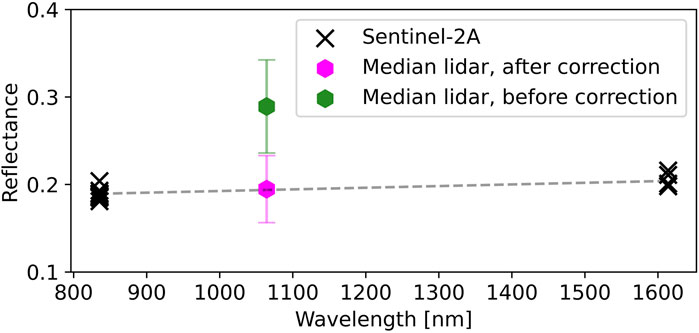
Figure 4. Reflectance of Sentinel-2A over the asphalt intersection in Eagle, Idaho (n = 9 pixels) with respect to computed median reflectance for lidar before and after applying the radiometric correction factor (n = 3,000) for 9 February 2023.

2.4.4 Estimating optical grain size from reflectance

Finally, reflectance for each flightline was rasterized from point cloud using the mean value per grid spacing of 0.5 m, and then resampled to 3 m spatial resolution using bilinear interpolation. We used a simplified version of the AART model (Kokhanovsky and Zege, 2004) with assumptions of zero dust concentration, 0% liquid water content, constant incidence angle due to normalizing in the previous step (μ = μ_s = μ_v = 1), and scattering angle ($\mathrm{\phi }$) as 180° (i.e., assuming direct backscattering direction) (Yang et al., 2017) (Table 2). The latter of these assumptions may potentially be a cause for error as AART is not well defined at 180°, and newer developments in BRDF kernels may be of use in future studies (Mei et al., 2022).

Table 2

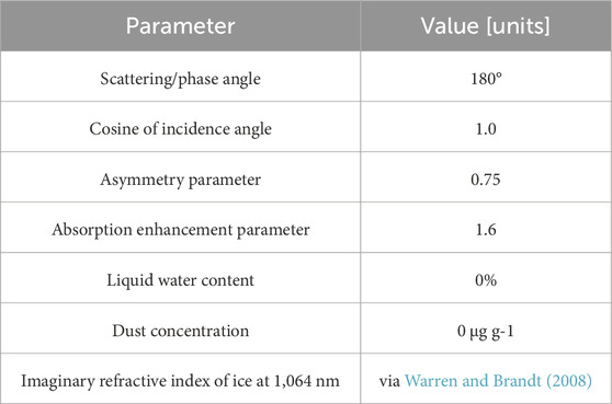
Table 2. Parameters used to build look-up table from AART model.

This allows us to solve Equation 8 to solve for $r0$ representing the semi-infinite non-absorbing snow layer,

$r0\left(\mathrm{\mu },\mathrm{\phi }\right)=\frac{1.247+1.186\left(2\mathrm{\mu }\right)+5.157{\mathrm{\mu }}^2+\left({11.1}^{\left(-0.087\mathrm{\phi }\right)}+{1.1}^{\left(-0.014\mathrm{\phi }\right)}\right)}{4\left(2\mathrm{\mu }\right)}(8)$

Given in our case that μ = 1 and $\mathrm{\phi }=180$, $r0$ is constant and is ≈1.108. The spherical albedo ($r_s$) can be estimated for clean, dry snow using the following Equation 9.

${r\left(\lambda \right)}_s={\exp }^{\left(-\sqrt{\left(\frac{4\pi k_{ice}\left(\lambda \right)}{\lambda }\right)\left(\xi d\right)}\right)}(9)$

where $d$ is the optical grain size diameter and $\xi$ is the grain shape parameter. Based on our parameters in Table 2, $\xi$ ≈11.38, which is the same value used in Kokhanovsky et al. (2018). Note that using other values for asymmetry parameter or absorption enhancement parameter will yield different values for $\xi$. We also know that $k_{ice}$ is a constant at 1,064 nm and can be plugged in. The resulting reflectance, ${\rho }_{snow}$, can be computed Equation 10.

${\rho }_{snow}=r0{\left[\exp \left(-\sqrt{\left(\frac{4\pi k_{ice}}{\lambda }\right)\left(\xi d\right)}\right)\right]}^f(10)$

where f is the escape function defined in Kokhanovsky et al. (2021). Because of the constants mentioned above, $f$ is also constant, and is ≈1.448. Therefore, we can rearrange Equations 9, 10 to yield the optical grain size radius, (i.e., d/2),

$radius=\frac{{\left\{\ln |\left({\left[\frac{{\rho }_{snow}}{r0}\right]}^{\frac{1}{f}}\right)\right\}}^2}{2\xi \left(\frac{4\pi k_{ice}}{\lambda }\right)}(11)$

We note that the resulting value in Equation 11 was multiplied by 1E6 to convert to μm. This derivation neglects any diffuse energy; however, given the active source lidar energy and low amount of diffuse solar energy at this 1,064 nm wavelength, we treat this effect as negligible. With these assumptions we were able to directly compute optical grain size radius from ${\rho }_{snow}$ at 1,064 nm and is demonstrated in Figure 5.

Figure 5

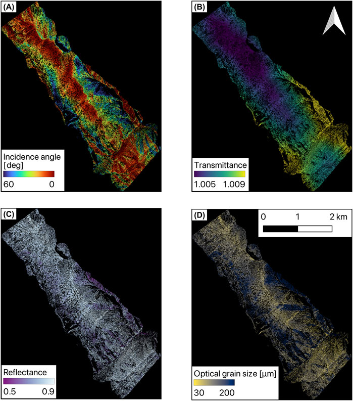
Figure 5. Subset of rasterized lidar retrievals for one flightline on 9 February 2023 including incidence angle (A), transmittance (B) calibrated reflectance (C), and optical grain size (D) at 3 m spatial resolution.

Important to note that both the asymmetry parameter and the absorption enhancement parameter were held constant between both the field estimates and the lidar estimates. We assumed grain shapes as constants, however, grain shape at the surface can vary spatially and temporally from snow redistribution and metamorphism (Fierz and Baunach, 2000). The assumption in this paper is that the grains are spheroid-like shapes, and homogeneous. However, for dry snow conditions, the temperature gradient and wind exposure play a large part in both variation of grain size and shape. We use similar grain shapes in both our field and lidar formulation, but different surface features (e.g., surface hoar), may present additional uncertainties not presented in this work.

2.5 Assessing uncertainties in reflectance and optical grain size

To assess temporal and spatial consistency of the calibrated reflectance across the three dates, we compared four surfaces that we assumed would have little change in the in-town site. These included a well-watered grass lot in a neighborhood, roof shingles on homes in a neighborhood, a concrete flat surface, and grass in golf course fairway. We also compared reference spectra at 1,064 nm (Meerdink et al., 2019) for these given surfaces.

We additionally computed the relative difference in reflectance between pixels from independent flightlines for the same date, to understand the precision in estimated reflectance. We performed a similar technique for the study site in the Boise National Forest and further compared these differences with respect to slope, to better understand uncertainties and how they varied across the landscape (Enderlin et al., 2022).

Finally, we computed the lidar-derived mean optical grain size for 10 m buffers surrounding our 9 field sampling locations to validate our method. Assuming each of the flightlines are independent, this increased our sample size to 28. Validation of grain size relies heavily on accuracy of the coincident snow-on DSM. As noted in previous work, even a ± 1° error in surface slope can greatly increase the error in retrieval of snow grain size from field spectroscopy (Tanikawa et al., 2020). In our case this also applies to the DSM-derived aspect. We do not know the absolute accuracy of our lidar derived slope and aspect maps, and thus to showcase how this may influence our retrieval, we have computed our uncertainty from spectroscopy inversions using ±0.01 of ${\mu }_s$.

2.6 Spatial and temporal relationships of lidar derived reflectance and optical grain size

To test how optical grain size varied spatially across the landscape, and to ensure the data products represented what we understand about interactions with terrain, we tested all pixels over all three dates with the corresponding snow-on elevation and Solar Radiation Index (SRI; Kane et al., 2008; Keating et al., 2007). The SRI co-variate is a function of slope, aspect, and latitude, and therefore provided information to test how optical grain size varied with respect to the amount of sunlight received by slopes for the day. Based on prior research, we assumed SRI closer to zero (i.e., shaded slopes) would have higher reflectance and smaller grains (Seidel et al., 2016). Then, we computed a distance to closest tree raster using our derived canopy height model and the Proximity Analysis tool in QGIS. Pixels were assumed to be canopy if the canopy height was at least 3 m or taller. Finally, we constructed simple linear regressions to determine the magnitude and direction of Pearson correlation of each of these co-variates for each flight based on a confidence interval of p = 0.05.

3 Results

3.1 Break point analysis of incidence angle

Using a break point analysis, we determined the optimal incidence angle where the signal was degraded (Figure 6). We found the best fit occurred with a break point of 42.0°, 68.5°, and 74.0° for the December, February, and March flights, respectively. This resulted in an average break point of 61.5° ($\mu$ = 0.48). Interestingly, the break point increased across the season and may be due in part to increased anisotropy for smaller grains (Painter and Dozier, 2004). To be conservative, and considering the added complexity of bright surfaces, we removed lidar returns where $\mu$ <0.5 (i.e., greater than 60°) in all our products (Ackroyd et al., 2024).

Figure 6

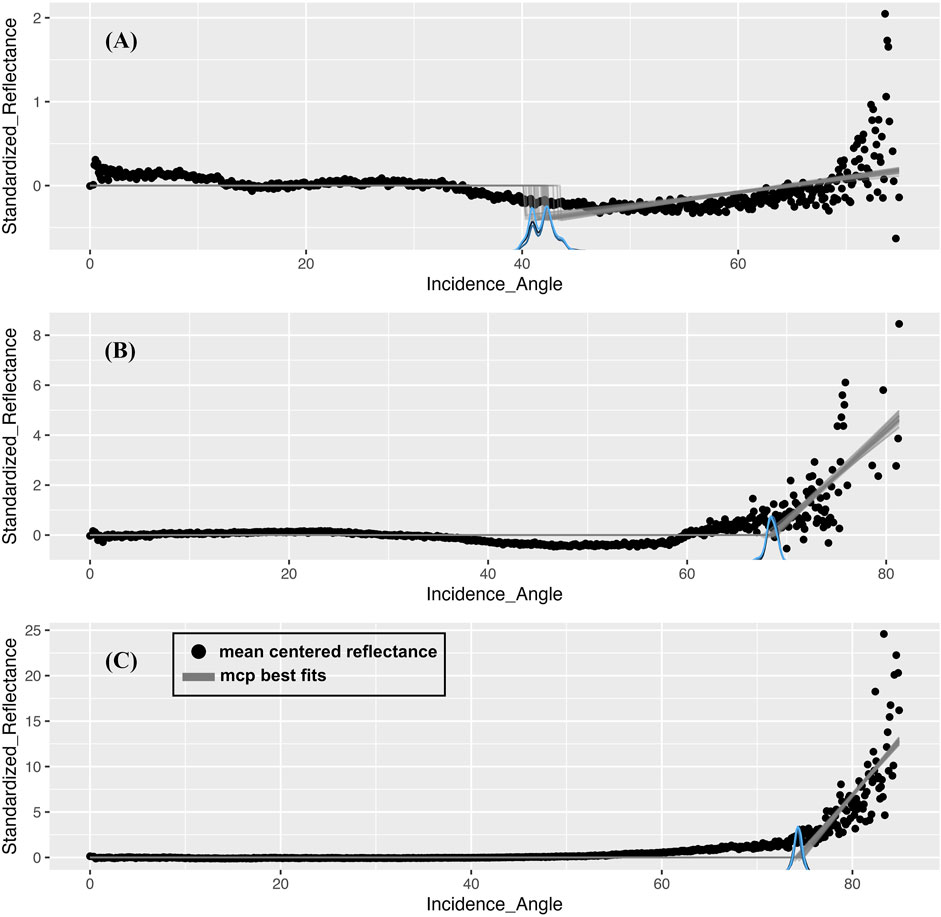
Figure 6. Breakpoint analysis for standardized reflectance (mean centered around 0) on the y-axis, and incidence angle (degrees) on the x-axis for each of the three flights, 8 December 2022 (A), 9 February 2023 (B), and 16 March 2023 (C). Grey lines and density distribution represent the derived uncertainty in the analysis from the MCP R package (Regression with Multiple Change Points).

3.2 Assessing retrieved reflectance in town

While we focused primarily on obtaining accurate snow reflectance measurements, we also used flightlines in-town in Eagle, Idaho, to ensure calibrated reflectance accurately represented other surfaces (Figure 7; Table 3). We followed a similar computational procedure; however, we did not resample to 3 m spatial resolution, and instead kept the DSM and reflectance data at 0.5 m resolution. This approach was reasonable because in-town surfaces were more variable at less than 3 m. When compared to reference spectra (Meerdink et al., 2019) and overlapping surfaces, calibrated reflectance values agreed across the season, especially for the housing shingles which varied only slightly from 0.06 to 0.08. When we compared two overlapping flightlines on 9 February 2023 at the flat, asphalt intersection, we found a mean absolute error of 0.016 (n = 2,432), which we interpreted as our in-town reflectance uncertainty over a flat surface. This uncertainty may help explain the differences we saw across the season in Table 3. Additionally, we observed high spatial variability in calibrated reflectance at 1,064 nm for asphalt (Figure 7), ranging from 0.04 to 0.30 across our flightline. This range represents different neighborhood developments with varying distributions of reflectance.

Figure 7

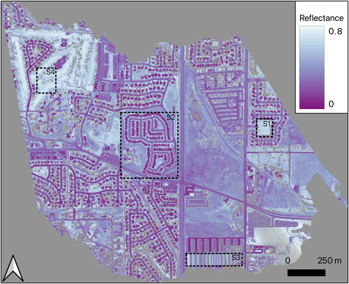
Figure 7. Estimated surface reflectance at 1,064 nm for Eagle, Idaho on 9 February 2023. Surfaces S1, S2, S3, and S4 represent grass, roof shingles, concrete, and grass at golf course, respectively (refer to Table 3).

Table 3

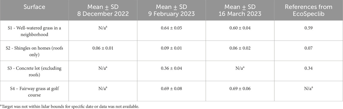
Table 3. Estimated surface reflectance at 1,064 nm for various surfaces in Eagle, Idaho with respect to reference reflectance from the literature. Pavement is not included in this table because it was used for calibration.

3.3 Assessing retrieved reflectance and optical grain size over Boise National Forest

Notable grain size patterns are demonstrated in Figure 5D. Steep, sunny slopes are shown with a darker blue that represents larger grain sizes. Also, on the north (top) side of the masked-out pixels from trees, grain sizes are variable, indicating sheltering of shortwave radiation from the canopy.

We found a median absolute difference in reflectance of 0.028 when comparing overlapping pixels over all slopes. There was some variability between bins with 0°-10° slopes having a difference of 0.025, 10°–20° slopes having a difference of 0.027, 20°–30° slopes having a difference of 0.029, 30°–40° slopes having a difference of 0.033, and slopes 40° or greater having a difference of 0.028 (Figure 8). In general, uncertainty in reflectance proportionally increased with slope.

Figure 8

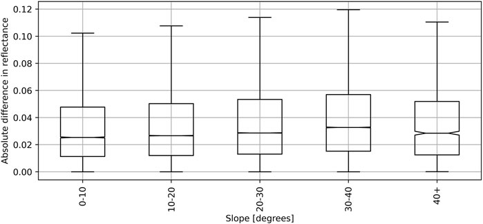
Figure 8. Boxplots of absolute difference in reflectance for overlapping pixels, where each boxplot is binned by slope bins.

When comparing field measurements to each of the flightlines directly, we found a RMSD = 49 μm, r = 0.57, and mean bias = +35 μm (n = 28, Figure 9). The percent mean absolute difference was computed to be 31%. For the February data, the median grain size from the ASD Fieldspec4 was 77 ± 36 μm, and median grain size from lidar at those same points was 115 ± 38 μm. For the one December data (ID-9), grain size from the ASD Fieldspec4 was computed to be 73 μm, and median grain size from lidar at the same point was 65 μm.

Figure 9

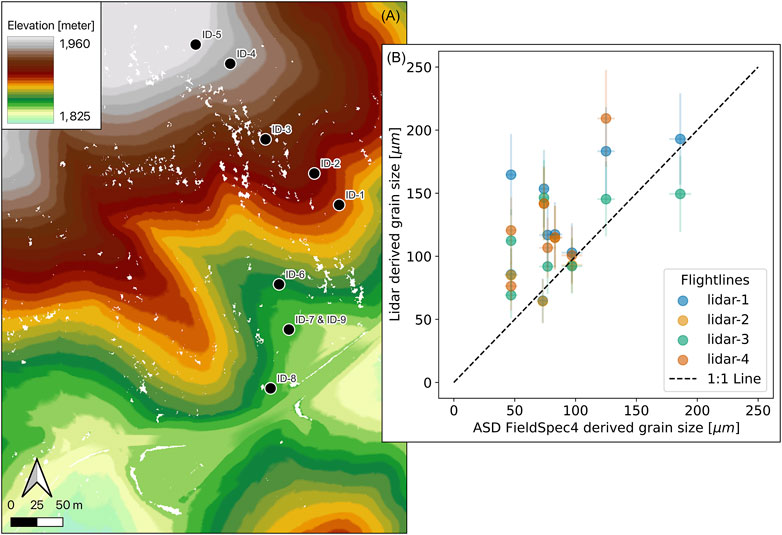
Figure 9. Map shown (A) with respect to our different samples from February flight (ID-1 through ID-8) and December flight (ID-9) (B). Uncertainties for lidar retrievals are shown by modeling ± 0.028 in reflectance (found in our study). Uncertainties for spectroscopy retrievals are shown by modeling ± 0.01 in cosine of the local solar illumination angle.

3.4 Spatial and temporal relationships of lidar derived reflectance and optical grain size

For the entire study domain reflectance values were generally higher earlier in the season, and lower later in the season, where median reflectance for 8 December 2022 was 0.84 ± 0.06, 9 February 2023 was 0.80 ± 0.07, and 16 March 2023 was 0.71 ± 0.06 (Figure 10). The largest change in reflectance occurred between the February and March flights. The optical grain size followed a similar temporal pattern (i.e., increasing grain growth as reflectance decreased), with the December flight having median optical grain size of 69 ± 65 μm, the February flight having a median optical grain size of 97 ± 81 μm, and the March flight having an optical grain size of 179 ± 90 μm.

Figure 10

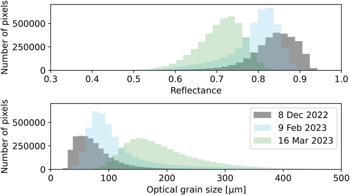
Figure 10. Histograms for all three flights showing the resulting snow reflectance (top) and optical grain size (bottom).

To understand the spatial relationship of different covariates (SRI, elevation, and distance to canopy) on optical grain size, we created simple linear regression models from all pixels. Most of the data were explained by SRI, where sunnier slopes had larger grains, and shadier slopes had smaller grains (Figure 11). However, this was not the case for the December flight at the beginning of the winter season where correlation was near zero (r = 0.02). Optical grain size from this flight seemed to be governed by the first winter storm where not enough time has passed for SRI to be a controlling factor. The effects from elevation are relatively smaller and similar across all flight dates, ranging from r = −0.22 to −0.31. This relationship shows a slight trend of larger grains at lower elevations within our study domain. Interestingly the distance to canopy metric had low explainability; however, for all three of the dates there was substantially more variability in optical grain size for pixels that were less than 30 m from canopy. Likewise, it appeared that the variation in retrieved grain size decreased with distance from tree cover.

Figure 11

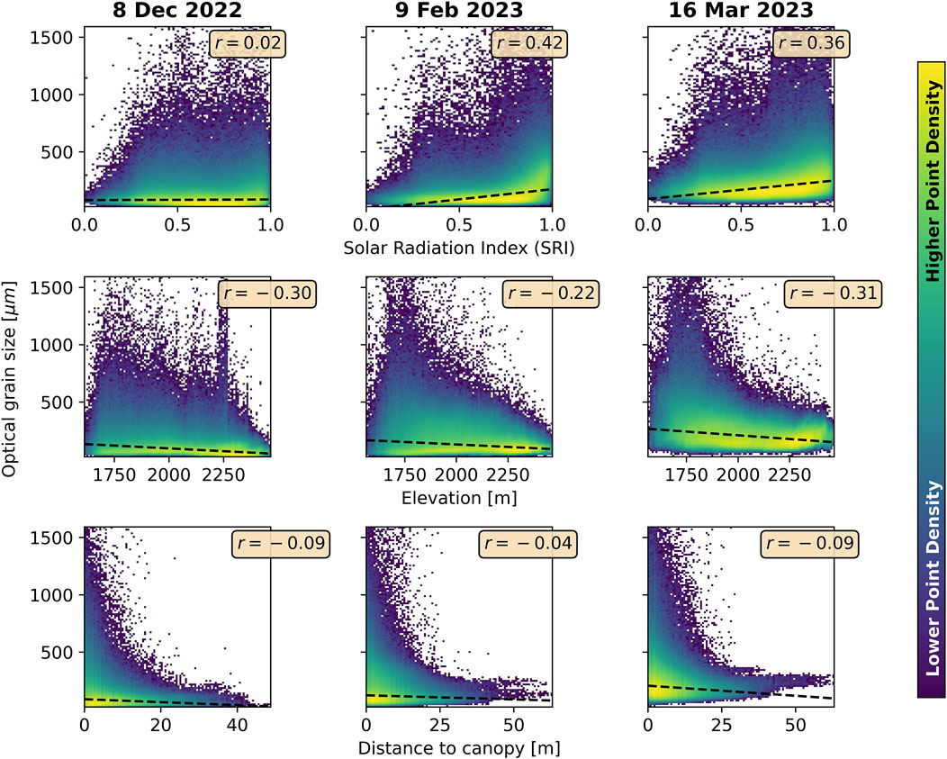
Figure 11. Linear regressions for testing the Pearson r coefficient for covariates SRI, elevation, and distance to canopy impacts on optical grain size for each of the three dates. Regressions were built using all data over study domain. Color scale shows log normalized point density, with lighter points having higher density and darker colors having lower density. All regressions were significant with p-values less than 0.01.

4 Discussion

4.1 Comparison of errors with other remote sensing methods and implications for future snow studies

In this study we introduced a workflow that used helicopter-borne lidar over the Boise National Forest to extract optical grain size with a RMSD of 49 μm. This accuracy is similar to Ackroyd et al. (2024) who used a similar approach and found a mean absolute error of 32 μm. The workflow presented here is similar to results from satellite spectroscopy (RMSE = 64 μm; Painter et al., 2009) and UAS spectroscopy (RMSE = 12 μm; Skiles et al., 2023) for clean, dry snow. However, as noted by Bohn et al. (2021), snow grain size retrieval for passive sensors dramatically decreases for solar zenith angles exceeding 45°. Therefore, it is plausible that accuracy of lidar in certain snow conditions may be beneficial for data fusion and/or calibration with retrieval methods from passive sensors. For example, it may be beneficial in a machine learning framework to combine optical grain size information from multiple sensors (Palomaki et al., 2024). Another example could be computing the surface normal from the raw radiance data of passive imaging spectroscopy datasets presents a novel development in snow retrieval in rugged terrain (Carmon et al., 2023; Wilder et al., 2024). Retrievals from lidar where the surface normal is accurately estimated may present a crucial validation source for these types of model developments, especially in the way we have catalogued the uncertainty with respect to terrain in this paper. Our method could also be used to improve modeling of grain size around canopies, which is one of the largest sources of uncertainty for passive sensors and is a major concern for global climate models. Using our method, and assumptions of dry, clean snow, we can retrieve snow optical properties in canopy gaps (Figure 12). With increasing changes in seasonal snow accumulation, it is important to understand the dynamics of optical grain size in greater detail so that snow property inversion may have higher certainty in challenging illumination conditions.

Figure 12

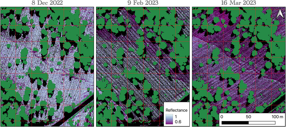
Figure 12. Demonstrating retrieval of snow reflectance at 1,064 nm at 0.5 m pixel resolution for a small portion of our study domain using one flightline. The trees are represented in green from our derived canopy height model. Red lines correspond to 30 m pixels typical for spaceborne passive sensors.

4.2 Limitations of this study and recommendations for developing this method further

While these results are encouraging, there are several opportunities to address in future studies. First and foremost, the presence of liquid water is a strict limitation on this method, preventing reliable results during the melt period. Mixed snow and liquid water manifests into the ice absorption feature widening and shifting towards shorter wavelengths (Green et al., 2006). Unfortunately, with a single wavelength (e.g., 1,064 nm), there is not enough information to resolve both liquid water content and optical grain size. However, this could be a potential opportunity for multi wavelength lidar (Niu et al., 2023).

Additionally, a large stable target of known reflectance (such as a large tarp) measured via field or airborne spectroscopy would be ideal (Ackroyd et al., 2024). We found a data fusion approach with coincident Sentinel-2A surface reflectance ( ±24 h) over a relatively stable target worked well and could be useful if large asphalt targets exist in the scene. However, the spatial variability and the relatively lower reflectance of asphalt may have manifested itself into a small bias in our results (Figure 9), suggesting that using a multi-surface calibration may work better. We proved this further by comparing the calibration factor by using our in situ data, yielding a calibration factor of 0.75 for both the December and February fights. This differs greatly from the Sentinel-2 calibration factor of 0.70 we found for February. This explains much of the positive bias we observed in Figure 9. Our work also assumed a linear response across a range of reflectance values; however, as shown in previous work this assumption may not hold when assessing low reflectance targets (roads) and high reflectance targets (snow) due to non-linearity in detector electronics (Calders et al., 2017).

Another alternative may be to use knowledge of the sensor’s emitted laser energy flux and the received radiance at sensor, which may be utilized to by-pass this radiometric bias correction (Yang et al., 2017). Unfortunately, emitted laser energy flux and radiance-at-sensor are not currently saved by Riegl instruments. If these data products were made available in the future, it would significantly progress the efficacy and accuracy in mapping snow properties from airborne lidar, specifically in eliminating radiometric bias and error–a key concern for solving optical properties from a single wavelength.

Small levels of uncertainty may also arise from our assumption that $a$ remained constant throughout each flight date. Water vapor is a major contributor to absorption at 1,064 nm (Yan et al., 2012) and any temporal variations would not be accounted for in the flights which could last a few hours. However, given the distance and elevation change between Eagle, Idaho, and Boise National Forest, it is possible that spatial and temporal differences in water column vapor and aerosol optical depth could introduce relatively small uncertainty in our reflectance estimation. Alternative approaches could be considered, such as using AERONET parameters for the radiometric calibration in Eagle, Idaho (due to the proximity), supplemented with coarser remote sensing data such as from the Geostationary Operational Environmental Satellite (GOES) (Fu et al., 2023).

The impact of incidence angle has been shown to be an essential parameter for estimating snow properties from lidar in mountain environments (Ackroyd et al., 2024), and while we took tremendous care in estimating incidence angles, there is room for improvement in our method. For example, we computed a DSM based on all flightlines for a given date; however, if some areas had lower point counts, this would dramatically reduce the reliability of the resulting slope and aspect grids. If this were a static surface, one could utilize the repeat flights to build a higher quality DSM, however, the snow surface is constantly changing at this site and is actively disturbed by snow machines and ski tracks. We also did not include points with incidence angles greater than 60° in the final processing step to reflectance. Past work has shown that correcting for incidence angle by dividing by $\mu$ can lead to overcorrections for large incidence angles (Yan and Shaker, 2014), and that another approach could be using a polynomial approximation to correct for incidence angle (Yan et al., 2017). Lidar collections with significant overlap between footprints and varying scan angles can enable more of these types of investigations.

4.3 Scalability of optical grain size retrievals for spaceborne applications

As demonstrated in the Yang et al. (2017) proof of concept study, optical grain size was retrieved over polar regions using the ICESAT GLAS instrument (1,064 nm). It is important to point out that while this worked for ICESAT, this methodology does not apply for ICESAT-2 (550 nm) which will inherently have less variability in reflectance due to changes in grain size. Presently, the Global Ecosystem Dynamics Investigation (GEDI) laser altimetry satellite mission collects at 1,064 nm although no grain size products have been published using this data source to date. The planned, Earth Dynamics Geodetic Explorer (EDGE), will also collect at this wavelength, as well as covering much of the cryosphere from 83° N to 83° S. This sensor may be well-suited for this application, as the assumption of low dust cover and low liquid water content may be met in high latitude regions. Future researchers may want to examine the efficacy of producing grain size retrievals from GEDI and other missions.

5 Conclusion

We present a method for estimating optical snow grain size from airborne lidar at 1,064 nm and assessed its accuracy over a winter in the Boise National Forest. We found reliable retrievals when compared to in situ measurements after conducting radiometric calibration with Sentinel-2A surface reflectance. When analyzing each flightline, we found that reflectance becomes unreliable as incidence angle increased. We ultimately used a 60° threshold for incidence angle in this study; however, another recent paper recommends a 40° threshold (Ackroyd et al., 2024). More work is needed to fully understand the limitations due to anisotropy of small grains and current BRDF models. Across the landscape we found optical grain size was primarily controlled by slope and aspect (which we documented here as SRI), with larger grains occurring on sunnier slopes. We also catalogued the uncertainty in airborne lidar derived snow reflectance with respect to slope. Our methodology and findings may help others progress the methods and science of accurately retrieving optical snow properties, especially in challenging illumination conditions.

Data availability statement

The raw lidar data is not currently available, but we are working on making it accessible in the future. Requests to access the datasets should be directed to BW, YnJlbnR3aWxkZXJAdS5ib2lzZXN0YXRlLmVkdQ==.

Author contributions

BW: Conceptualization, Data curation, Formal Analysis, Funding acquisition, Investigation, Methodology, Resources, Software, Validation, Visualization, Writing–original draft, Writing–review and editing. JE: Conceptualization, Data curation, Formal Analysis, Funding acquisition, Investigation, Methodology, Project administration, Resources, Software, Supervision, Validation, Visualization, Writing–original draft, Writing–review and editing. ZH: Data curation, Formal Analysis, Investigation, Methodology, Software, Validation, Visualization, Writing–original draft, Writing–review and editing. NA: Data curation, Formal Analysis, Investigation, Methodology, Software, Validation, Visualization, Writing–original draft, Writing–review and editing. H-PM: Formal Analysis, Investigation, Methodology, Resources, Supervision, Visualization, Writing–original draft, Writing–review and editing. SO’N: Data curation, Funding acquisition, Investigation, Methodology, Project administration, Resources, Software, Supervision, Writing–original draft, Writing–review and editing. TV: Data curation, Methodology, Writing–original draft, Writing–review and editing. AK: Writing–original draft, Writing–review and editing. NG: Conceptualization, Funding acquisition, Investigation, Project administration, Resources, Supervision, Writing–original draft, Writing–review and editing.

Funding

The author(s) declare that financial support was received for the research, authorship, and/or publication of this article. This research has been supported by FINESST Award – 21-EARTH21-0249.

Acknowledgments

The authors would like to thank Dominic Filiano and Nani Ciafone from Cold Regions Research and Engineering Laboratory and Karina Zikan and the rest of the Boise State lidar team for their work planning, collecting, and processing this dataset. The authors also acknowledge staff from the Boise National Forest for their cooperation in data collection, and Silverhawk Aviation Academy for piloting the missions. Last but not least, the authors acknowledge and thank Chelsea Ackroyd and McKenzie Skiles for sharing snow grain size from lidar methods at the Western Snow Conference 2022 in Salt Lake City, Utah.

Conflict of interest

The authors declare that the research was conducted in the absence of any commercial or financial relationships that could be construed as a potential conflict of interest.

Publisher’s note

All claims expressed in this article are solely those of the authors and do not necessarily represent those of their affiliated organizations, or those of the publisher, the editors and the reviewers. Any product that may be evaluated in this article, or claim that may be made by its manufacturer, is not guaranteed or endorsed by the publisher.

Supplementary material

The Supplementary Material for this article can be found online at: https://www.frontiersin.org/articles/10.3389/feart.2025.1487776/full#supplementary-material

References

Ackroyd, C., Donahue, C. P., Menounos, B., and Skiles, S. M. (2024). Airborne lidar intensity correction for mapping snow cover extent and effective grain size in mountainous terrain. GI Science and Remote Sens. 61 (1), 2427326. doi:10.1080/15481603.2024.2427326

CrossRef Full Text | Google Scholar

Adebisi, N., Marshall, H., O'Neel, S., Vuyovich, C. M., Hiemstra, C., and Elder, K. (2022). SnowEx20-21 QSI lidar DEM 0.5m UTM grid, version 1. NASA Natl. Snow Ice Data Cent. Distributed Act. Archive Cent. doi:10.5067/YO583L7ZOLOO

CrossRef Full Text | Google Scholar

Bair, E. H., Stillinger, T., and Dozier, J. (2020). Snow property inversion from remote sensing (SPIReS): a generalized multispectral unmixing approach with examples from MODIS and landsat 8 oli. IEEE Trans. Geoscience Remote Sens. 59 (9), 7270–7284. doi:10.1109/TGRS.2020.3040328

CrossRef Full Text | Google Scholar

Barnett, T. P., Adam, J. C., and Lettenmaier, D. P. (2005). Potential impacts of a warming climate on water availability in snow-dominated regions. Nature 438 (7066), 303–309. doi:10.1038/nature04141

PubMed Abstract | CrossRef Full Text | Google Scholar

Beyer, R. A., Alexandrov, O., and McMichael, S. (2018). The Ames Stereo Pipeline: NASA’s open source software for deriving and processing terrain data. Earth Space Sci. 5 (9), 537–548. doi:10.1029/2018EA000409

CrossRef Full Text | Google Scholar

Bohn, N., Painter, T. H., Thompson, D. R., Carmon, N., Susiluoto, J., Turmon, M. J., et al. (2021). Optimal estimation of snow and ice surface parameters from imaging spectroscopy measurements. Remote Sens. Environ. 264, 112613. doi:10.1016/j.rse.2021.112613

CrossRef Full Text | Google Scholar

Briese, C., Pfennigbauer, M., Lehner, H., Ullrich, A., Wagner, W., and Pfeifer, N. (2012). Radiometric calibration of multi-wavelength airborne laser scanning data. ISPRS Ann. Photogrammetry, Remote Sens. Spatial Inf. Sci. 1, 335–340. doi:10.5194/isprsannals-I-7-335-2012

CrossRef Full Text | Google Scholar

Calders, K., Disney, M. I., Armston, J., Burt, A., Brede, B., Origo, N., et al. (2017). Evaluation of the range accuracy and the radiometric calibration of multiple terrestrial laser scanning instruments for data interoperability. IEEE Trans. Geoscience Remote Sens. 55 (5), 2716–2724. doi:10.1109/tgrs.2017.2652721

CrossRef Full Text | Google Scholar

Carmon, N., Berk, A., Bohn, N., Brodrick, P. G., Dozier, J., Johnson, M., et al. (2023). Shape from spectra. Remote Sens. Environ. 288, 113497. doi:10.1016/j.rse.2023.113497

CrossRef Full Text | Google Scholar

Cawse-Nicholson, K., Townsend, P. A., Schimel, D., Assiri, A. M., Blake, P. L., Buongiorno, M. F., et al. (2021). NASA's surface biology and geology designated observable: a perspective on surface imaging algorithms. Remote Sens. Environ. 257, 112349. doi:10.1016/j.rse.2021.112349

CrossRef Full Text | Google Scholar

Cogliati, S., Sarti, F., Chiarantini, L., Cosi, M., Lorusso, R., Lopinto, E., et al. (2021). The PRISMA imaging spectroscopy mission: overview and first performance analysis. Remote Sens. Environ. 262, 112499. doi:10.1016/j.rse.2021.112499

CrossRef Full Text | Google Scholar

Colbeck, S. C. (1982). An overview of seasonal snow metamorphism. Rev. Geophys. 20 (1), 45–61. doi:10.1029/RG020i001p00045

CrossRef Full Text | Google Scholar

Dowle, M., Srinivasan, A., Gorecki, J., Chirico, M., Stetsenko, P., Short, T., et al. (2019). Package “data. table”. Extension of ‘data. frame, 596.

Google Scholar

Dozier, J., Bair, E. H., Baskaran, L., Brodrick, P. G., Carmon, N., Kokaly, R. F., et al. (2022). Error and uncertainty degrade topographic corrections of remotely sensed data. J. Geophys. Res. Biogeosciences 127 (11), e2022JG007147. doi:10.1029/2022JG007147

CrossRef Full Text | Google Scholar

Dozier, J., and Painter, T. H. (2004). Multispectral and hyperspectral remote sensing of alpine snow properties. Annu. Rev. Earth Planet. Sci. 32, 465–494. doi:10.1146/annurev.earth.32.101802.120404

CrossRef Full Text | Google Scholar

Durand, M., and Margulis, S. A. (2008). Effects of uncertainty magnitude and accuracy on assimilation of multiscale measurements for snowpack characterization. J. Geophys. Res. Atmos. 113 (D2). doi:10.1029/2007JD008662

PubMed Abstract | CrossRef Full Text | Google Scholar

Enderlin, E. M., Elkin, C. M., Gendreau, M., Marshall, H. P., O'Neel, S., McNeil, C., et al. (2022). Uncertainty of ICESat-2 ATL06-and ATL08-derived snow depths for glacierized and vegetated mountain regions. Remote Sens. Environ. 283, 113307. doi:10.1016/j.rse.2022.113307

CrossRef Full Text | Google Scholar

Fair, Z., Flanner, M., Schneider, A., and Skiles, S. M. (2022). Sensitivity of modeled snow grain size retrievals to solar geometry, snow particle asphericity, and snowpack impurities. Cryosphere 16 (9), 3801–3814. doi:10.5194/tc-16-3801-2022

CrossRef Full Text | Google Scholar

Fierz, C., and Baunach, T. (2000). Quantifying grain-shape changes in snow subjected to large temperature gradients. Ann. Glaciol. 31, 439–444. doi:10.3189/172756400781820516

CrossRef Full Text | Google Scholar

Fu, D., Gueymard, C. A., and Xia, X. (2023). Validation of the improved GOES-16 aerosol optical depth product over North America. Atmos. Environ. 298, 119642. doi:10.1016/j.atmosenv.2023.119642

CrossRef Full Text | Google Scholar

Gallet, J. C., Domine, F., Zender, C. S., and Picard, G. (2009). Measurement of the specific surface area of snow using infrared reflectance in an integrating sphere at 1310 and 1550 nm. Cryosphere 3 (2), 167–182. doi:10.5194/tc-3-167-2009

CrossRef Full Text | Google Scholar

Gay, M., Fily, M., Genthon, C., Frezzotti, M., Oerter, H., and Winther, J. G. (2002). Snow grain-size measurements in Antarctica. J. Glaciol. 48 (163), 527–535. doi:10.3189/172756502781831016

CrossRef Full Text | Google Scholar

Green, R. O., Painter, T. H., Roberts, D. A., and Dozier, J. (2006). Measuring the expressed abundance of the three phases of water with an imaging spectrometer over melting snow. Water Resour. Res. 42 (10). doi:10.1029/2005WR004509

CrossRef Full Text | Google Scholar

Harpold, A. A. (2016). Diverging sensitivity of soil water stress to changing snowmelt timing in the Western US. Adv. Water Resour. 92, 116–129. doi:10.1016/j.advwatres.2016.03.017

CrossRef Full Text | Google Scholar

He, C., Takano, Y., Liou, K. N., Yang, P., Li, Q., and Chen, F. (2017). Impact of snow grain shape and black carbon–snow internal mixing on snow optical properties: parameterizations for climate models. J. Clim. 30 (24), 10019–10036. doi:10.1175/JCLI-D-17-0300.1

CrossRef Full Text | Google Scholar

Herold, M. (2004). Understanding spectral characteristics of asphalt roads. Santa Barbara: University of California. National Center for Remote Sensing in Transportation.

Google Scholar

Herold, M., and Roberts, D. (2005). Spectral characteristics of asphalt road aging and deterioration: implications for remote-sensing applications. Appl. Opt. 44 (20), 4327–4334. doi:10.1364/AO.44.004327

PubMed Abstract | CrossRef Full Text | Google Scholar

Herold, M., Roberts, D., Noronha, V., and Smadi, O. (2008). Imaging spectrometry and asphalt road surveys. Transp. Res. Part C Emerg. Technol. 16 (2), 153–166. doi:10.1016/j.trc.2007.07.001

CrossRef Full Text | Google Scholar

Hoppinen, Z., Wilder, B., O’Neel, S., and Adebisi, N. (2023). SnowEx/ice-road-copters: v1.0.0 (v1.0.0). Zenodo. doi:10.5281/zenodo.8184592

CrossRef Full Text | Google Scholar

Kane, V. R., Gillespie, A. R., McGaughey, R., Lutz, J. A., Ceder, K., and Franklin, J. F. (2008). Interpretation and topographic compensation of conifer canopy self-shadowing. Remote Sens. Environ. 112 (10), 3820–3832. doi:10.1016/j.rse.2008.06.001

CrossRef Full Text | Google Scholar

Keating, K. A., Gogan, P. J., Vore, J. M., and Irby, L. R. (2007). A simple solar radiation index for wildlife habitat studies. J. Wildl. Manag. 71 (4), 1344–1348. doi:10.2193/2006-359

CrossRef Full Text | Google Scholar

Klein, A. G., Hall, D. K., and Riggs, G. A. (1998). Improving snow cover mapping in forests through the use of a canopy reflectance model. Hydrol. Process. 12 (10-11), 1723–1744. doi:10.1002/(sici)1099-1085(199808/09)12:10/11<1723::aid-hyp691>3.0.co;2-2

CrossRef Full Text | Google Scholar

Kokhanovsky, A., Di Mauro, B., Garzonio, R., and Colombo, R. (2021). Retrieval of dust properties from spectral snow reflectance measurements. Front. Environ. Sci. 9, 644551. doi:10.3389/fenvs.2021.644551

CrossRef Full Text | Google Scholar

Kokhanovsky, A., Lamare, M., Di Mauro, B., Picard, G., Arnaud, L., Dumont, M., et al. (2018). On the reflectance spectroscopy of snow. Cryosphere 12 (7), 2371–2382. doi:10.5194/tc-12-2371-2018

CrossRef Full Text | Google Scholar

Kokhanovsky, A. A., Brell, M., Segl, K., Bianchini, G., Lanconelli, C., Lupi, A., et al. (2023). First retrievals of surface and atmospheric properties using EnMAP measurements over Antarctica. Remote Sens. 15 (12), 3042. doi:10.3390/rs15123042

CrossRef Full Text | Google Scholar

Kokhanovsky, A. A., and Zege, E. P. (2004). Scattering optics of snow. Appl. Opt. 43 (7), 1589–1602. doi:10.1364/AO.43.001589

PubMed Abstract | CrossRef Full Text | Google Scholar

Kraft, D. (1988). “A software package for sequential quadratic programming,” in Forschungsbericht- Deutsche Forschungs-und Versuchsanstalt fur Luft-und Raumfahrt.

Google Scholar

Libois, Q., Picard, G., France, J. L., Arnaud, L., Dumont, M., Carmagnola, C. M., et al. (2013). Influence of grain shape on light penetration in snow. Cryosphere 7 (6), 1803–1818. doi:10.5194/tc-7-1803-2013

CrossRef Full Text | Google Scholar

Lindeløv, J. K. (2020). mcp: an R package for regression with multiple change points.

Google Scholar

Liu, J., Melloh, R. A., Woodcock, C. E., Davis, R. E., and Ochs, E. S. (2004). The effect of viewing geometry and topography on viewable gap fractions through forest canopies. Hydrol. Process. 18 (18), 3595–3607. doi:10.1002/hyp.5802

CrossRef Full Text | Google Scholar

Mayer, B., and Kylling, A. (2005). Technical note: the libRadtran software package for radiative transfer calculations - description and examples of use. Atmos. Chem. Phys. 5 (7), 1855–1877. doi:10.5194/acp-5-1855-2005

CrossRef Full Text | Google Scholar

Meerdink, S. K., Hook, S. J., Roberts, D. A., and Abbott, E. A. (2019). The ECOSTRESS spectral library version 1.0. Remote Sens. Environ. 230, 111196. doi:10.1016/j.rse.2019.05.015

CrossRef Full Text | Google Scholar

Mei, L., Rozanov, V., Jiao, Z., and Burrows, J. P. (2022). A new snow bidirectional reflectance distribution function model in spectral regions from UV to SWIR: model development and application to ground-based, aircraft and satellite observations. ISPRS J. Photogrammetry Remote Sens. 188, 269–285. doi:10.1016/j.isprsjprs.2022.04.010

CrossRef Full Text | Google Scholar

Miller, S. D., Wang, F., Burgess, A. B., Skiles, S. M., Rogers, M., and Painter, T. H. (2016). Satellite-based estimation of temporally resolved dust radiative forcing in snow cover. J. Hydrometeorol. 17 (7), 1999–2011. doi:10.1175/JHM-D-15-0150.1

CrossRef Full Text | Google Scholar

Montpetit, B., Royer, A., Langlois, A., Cliche, P., Roy, A., Champollion, N., et al. (2012). New shortwave infrared albedo measurements for snow specific surface area retrieval. J. Glaciol. 58 (211), 941–952. doi:10.3189/2012JoG11J248

CrossRef Full Text | Google Scholar

Muhuri, A., Gascoin, S., Menzel, L., Kostadinov, T. S., Harpold, A. A., Sanmiguel-Vallelado, A., et al. (2021). Performance assessment of optical satellite-based operational snow cover monitoring algorithms in forested landscapes. IEEE J. Sel. Top. Appl. Earth Observations Remote Sens. 14, 7159–7178. doi:10.1109/JSTARS.2021.3089655

CrossRef Full Text | Google Scholar

Nolin, A. W. (2010). Recent advances in remote sensing of seasonal snow. J. Glaciol. 56 (200), 1141–1150. doi:10.3189/002214311796406077

CrossRef Full Text | Google Scholar

Nolin, A. W., and Dozier, J. (1993). Estimating snow grain size using AVIRIS data. Remote Sens. Environ. 44 (2-3), 231–238. doi:10.1016/0034-4257(93)90018-S

CrossRef Full Text | Google Scholar

Nolin, A. W., and Dozier, J. (2000). A hyperspectral method for remotely sensing the grain size of snow. Remote Sens. Environ. 74 (2), 207–216. doi:10.1016/S0034-4257(00)00111-5

CrossRef Full Text | Google Scholar

O'Neel, S., Wilder, B., Keskinen, Z., Zikan, K. H., Enterkine, J., Filiano, D. L., et al. (2022). Helicopter-borne lidar to resolve snowpack variability in Southwest Idaho. AGU Fall Meet. Abstr. 2022, C35E–C0922.

Google Scholar

Painter, T. H., Berisford, D. F., Boardman, J. W., Bormann, K. J., Deems, J. S., Gehrke, F., et al. (2016). The Airborne Snow Observatory: fusion of scanning lidar, imaging spectrometer, and physically-based modeling for mapping snow water equivalent and snow albedo. Remote Sens. Environ. 184, 139–152. doi:10.1016/j.rse.2016.06.018

CrossRef Full Text | Google Scholar

Painter, T. H., and Dozier, J. (2004). The effect of anisotropic reflectance on imaging spectroscopy of snow properties. Remote Sens. Environ. 89 (4), 409–422. doi:10.1016/j.rse.2003.09.007

CrossRef Full Text | Google Scholar

Painter, T. H., Molotch, N. P., Cassidy, M., Flanner, M., and Steffen, K. (2007). Contact spectroscopy for determination of stratigraphy of snow optical grain size. J. Glaciol. 53 (180), 121–127. doi:10.3189/172756507781833947

CrossRef Full Text | Google Scholar

Painter, T. H., Rittger, K., McKenzie, C., Slaughter, P., Davis, R. E., and Dozier, J. (2009). Retrieval of subpixel snow covered area, grain size, and albedo from MODIS. Remote Sens. Environ. 113 (4), 868–879. doi:10.1016/j.rse.2009.01.001

CrossRef Full Text | Google Scholar

Painter, T. H., Seidel, F. C., Bryant, A. C., McKenzie Skiles, S., and Rittger, K. (2013). Imaging spectroscopy of albedo and radiative forcing by light-absorbing impurities in mountain snow. J. Geophys. Res. Atmos. 118 (17), 9511–9523. doi:10.1002/jgrd.50520

CrossRef Full Text | Google Scholar

Palomaki, R. T., Rittger, K., Lenard, S. J., Dozier, J., and Skiles, S. M. (2024). A data fusion approach to produce daily, high resolution snow albedo using multispectral and hyperspectral imagery. Copernic. Meet.

Google Scholar

PDAL Contributors (2022). PDAL point data abstraction library. doi:10.5281/zenodo.2616780

CrossRef Full Text | Google Scholar

Räisänen, P., Makkonen, R., Kirkevåg, A., and Debernard, J. B. (2017). Effects of snow grain shape on climate simulations: sensitivity tests with the Norwegian Earth System Model. Cryosphere 11 (6), 2919–2942. doi:10.5194/tc-11-2919-2017

CrossRef Full Text | Google Scholar

Raleigh, M. S., Rittger, K., Moore, C. E., Henn, B., Lutz, J. A., and Lundquist, J. D. (2013). Ground-based testing of MODIS fractional snow cover in subalpine meadows and forests of the Sierra Nevada. Remote Sens. Environ. 128, 44–57. doi:10.1016/j.rse.2012.09.016

CrossRef Full Text | Google Scholar

Riegl (2017). LAS extrabytes implementation in RIEGL software. Available at: http://www.riegl.com/uploads/tx_pxpriegldownloads/RIEGL_VQ-580II_Datasheet_2024-02-13.pdf.

Google Scholar

Roussel, J., and Auty, D. (2023). Airborne lidar data manipulation and visualization for forestry applications. R. package version 4.0.4. Available at: https://cran.r-project.org/package=lidR.

Google Scholar

Roussel, J., Auty, D., Coops, N. C., Tompalski, P., Goodbody, T. R., Meador, A. S., et al. (2020). lidR: an R package for analysis of Airborne Laser Scanning (ALS) data. Remote Sens. Environ. 251, 112061. doi:10.1016/j.rse.2020.112061

CrossRef Full Text | Google Scholar

Roussel, J., and De Boissieu, F. (2023). _rlas: read and write 'las' and 'Laz' binary file formats used for remote sensing data_. R. package version 1.6.3. Available at: https://CRAN.R-project.org/package=rlas.

Google Scholar

Seidel, F. C., Rittger, K., Skiles, S. M., Molotch, N. P., and Painter, T. H. (2016). Case study of spatial and temporal variability of snow cover, grain size, albedo and radiative forcing in the Sierra Nevada and Rocky Mountain snowpack derived from imaging spectroscopy. Cryosphere 10 (3), 1229–1244. doi:10.5194/tc-10-1229-2016

CrossRef Full Text | Google Scholar

Skiles, S. M., Donahue, C. P., Hunsaker, A. G., and Jacobs, J. M. (2023). UAV hyperspectral imaging for multiscale assessment of Landsat 9 snow grain size and albedo. Front. Remote Sens. 3, 1038287. doi:10.3389/frsen.2022.1038287

CrossRef Full Text | Google Scholar

Stillinger, T., Rittger, K., Raleigh, M. S., Michell, A., Davis, R. E., and Bair, E. H. (2023). Landsat, MODIS, and VIIRS snow cover mapping algorithm performance as validated by airborne lidar datasets. Cryosphere 17 (2), 567–590. doi:10.5194/tc-17-567-2023

CrossRef Full Text | Google Scholar

Sturm, M., Goldstein, M. A., and Parr, C. (2017). Water and life from snow: a trillion dollar science question. Water Resour. Res. 53 (5), 3534–3544. doi:10.1002/2017WR020840

CrossRef Full Text | Google Scholar

Swinehart, D. F. (1962). The beer-lambert law. J. Chem. Educ. 39 (7), 333. doi:10.1021/ed039p333

CrossRef Full Text | Google Scholar

Tanikawa, T., Kuchiki, K., Aoki, T., Ishimoto, H., Hachikubo, A., Niwano, M., et al. (2020). Effects of snow grain shape and mixing state of snow impurity on retrieval of snow physical parameters from ground-based optical instrument. J. Geophys. Res. Atmos. 125 (15), e2019JD031858. doi:10.1029/2019JD031858

CrossRef Full Text | Google Scholar

Thompson, D. R., Green, R. O., Bradley, C., Brodrick, P. G., Mahowald, N., Dor, E. B., et al. (2024). On-orbit calibration and performance of the EMIT imaging spectrometer. Remote Sens. Environ. 303, 113986. doi:10.1016/j.rse.2023.113986

CrossRef Full Text | Google Scholar

Uecker, T. M., Kaspari, S. D., Musselman, K. N., and Skiles, S. M. (2020). The post-wildfire impact of burn severity and age on black carbon snow deposition and implications for snow water resources, cascade range, Washington. J. Hydrometeorol. 21 (8), 1777–1792. doi:10.1175/JHM-D-20-0010.1

CrossRef Full Text | Google Scholar

Vikhamar, D., and Solberg, R. (2003). Snow-cover mapping in forests by constrained linear spectral unmixing of MODIS data. Remote Sens. Environ. 88 (3), 309–323. doi:10.1016/j.rse.2003.06.004

CrossRef Full Text | Google Scholar

Warren, S. G. (1982). Optical properties of snow. Rev. Geophys. 20 (1), 67–89. doi:10.1029/RG020i001p00067

CrossRef Full Text | Google Scholar

Warren, S. G., and Brandt, R. E. (2008). Optical constants of ice from the ultraviolet to the microwave: a revised compilation. J. Geophys. Res. Atmos. 113 (D14). doi:10.1029/2007JD009744

PubMed Abstract | CrossRef Full Text | Google Scholar

Warren, S. G., and Wiscombe, W. J. (1980). A model for the spectral albedo of snow. II: snow containing atmospheric aerosols. J. Atmos. Sci. 37 (12), 2734–2745. doi:10.1175/1520-0469(1980)037<2734:amftsa>2.0.co;2

CrossRef Full Text | Google Scholar

Wilder, B. A., Meyer, J., Enterkine, J., and Glenn, N. F. (2024). Improved snow property retrievals by solving for topography in the inversion of at-sensor radiance measurements. Cryosphere 18 (11), 5015–5029. doi:10.5194/tc-18-5015-2024

CrossRef Full Text | Google Scholar

Wu, Q., Zhong, R., Dong, P., Mo, Y., and Jin, Y. (2021). Airborne lidar intensity correction based on a new method for incidence angle correction for improving land-cover classification. Remote Sens. 13 (3), 511. doi:10.3390/rs13030511

CrossRef Full Text | Google Scholar

Yan, W. Y., and Shaker, A. (2014). Radiometric correction and normalization of airborne Lidar intensity data for improving land-cover classification. IEEE Trans. Geoscience Remote Sens. 52 (12), 7658–7673. doi:10.1109/TGRS.2014.2316195

CrossRef Full Text | Google Scholar

Yan, W. Y., and Shaker, A. (2017). Correction of overlapping multispectral lidar intensity data: polynomial approximation of range and angle effects. Int. Archives Photogrammetry, Remote Sens. Spatial Inf. Sci. 42, 177–182. doi:10.5194/isprs-archives-XLII-3-W1-177-2017

CrossRef Full Text | Google Scholar

Yan, W. Y., Shaker, A., Habib, A., and Kersting, A. P. (2012). Improving classification accuracy of airborne Lidar intensity data by geometric calibration and radiometric correction. ISPRS J. Photogrammetry Remote Sens. 67, 35–44. doi:10.1016/j.isprsjprs.2011.10.005

CrossRef Full Text | Google Scholar

Yang, Y., Marshak, A., Han, M., Palm, S. P., and Harding, D. J. (2017). Snow grain size retrieval over the polar ice sheets with the Ice, Cloud, and land Elevation Satellite (ICESat) observations. J. Quantitative Spectrosc. Radiat. Transf. 188, 159–164. doi:10.1016/j.jqsrt.2016.03.033

PubMed Abstract | CrossRef Full Text | Google Scholar

Zuanon, N. (2013). “IceCube, a portable and reliable instruments for snow specific surface area measurement in the field,” in International snow science workshop grenoble-chamonix mont-blance-2013 proceedings, 1020–1023.

Google Scholar

Appendix 1

ASD FieldSpec4 Data

We have included our location, terrain, and grain size estimates from field spectroscopy in Table A1.

Table A1

TABLE A1. Location, terrain, and grain size estimates for each ground measurement.