Comparative analysis of formulations for crossed artifact elimination in the frequency–Bessel spectrograms

The frequency–Bessel transformation method has significantly advanced the extraction of multimodal surface waves in seismic research. However, the presence of crossed artifacts in frequency–Bessel spectrograms, particularly when stations are regularly distributed, presents a persistent challenge. Various methods have been proposed to mitigate these artifacts, yet their diverse formulations often lead to confusion about their practical application and interrelations. This study aims to demystify these ambiguities by analyzing the existing formulations within a unified framework. We uncover that the apparent discrepancies among these methods primarily originate from the differing conventions across various studies. Consequently, we establish explicit mathematical relationships among these existing formulations. Moreover, we demonstrate that the reliance on numerical Hilbert transform can be avoided by maintaining only the causal component of cross-correlation functions. This approach simplifies the artifact removal process, enhancing the practical utility of frequency–Bessel spectrograms in geophysical analysis.

1 Introduction

Since the introduction of the frequency–Bessel transformation (FJ) method to extract multimodal surface wave dispersion curves by Wang et al. (2019) and Forbriger (2003), it is shortly recognized that crossed artifacts appear in the spectrograms when the stations are regularly distributed. Forbriger (2003) suggested that these artifacts could be reduced to use the Hankel function instead of the Bessel function in the integration process. Following this, subsequent studies by Xi et al. (2021), Luo et al. (2022), Zhou et al. (2023), and Yang et al. (2024) have explored diverse strategies to address this issue.

However, Yang et al. (2024) highlighted that there is a lack of consistency among these methods. For example, Forbriger (2003) and Xi et al. (2021) used $H_0^{(2)}$ in their formulations, while Luo et al. (2022) and Yang et al. (2024) preferred $H_0^{(1)}$. Additionally, Luo et al. (2022) did not explicitly include the Hilbert transform, which is a requirement in other studies. This disparity raises questions about which method is most effective in practice, whether these methods are fundamentally similar, and how they are related.

In this paper, we show how to extend Forbriger (2003)’s formulation from active to passive sources. We then analyze different approaches, focusing on the works by Forbriger (2003), Xi et al. (2021), Luo et al. (2022), Zhou et al. (2023), and Yang et al. (2024), using a consistent convention, and explore the relationships among these studies. We also make some clarifications on our previous study (Luo et al., 2022) and show how the usage of the numerical Hilbert transform can be avoided.

2 Theory

2.1 Conventions

We use the Hilbert transform in the form (Hahn, 1996)

$\mathcal{H}\left[f\right]\left(\omega \right)=\frac{1}{\pi }\text{P}{\int }_{-\infty }^{\infty }\frac{f\left({\omega }^{\prime }\right)}{\omega -{\omega }^{\prime }}\mathrm{d}{\omega }^{\prime },(1)$

where the symbol P denotes the Cauchy principal value. This definition aligns with current literature (Hahn, 1996; Johnansson, 1999) and is implemented in the MATLAB software and the Python function scipy.signal.hilbert. However, it differs in sign from the definition of Erdelyi (1954) and the Python function scipy.fftpack.hilbert. According to Hu (1989), as cited by Zhou and Chen (2021) and Yang et al. (2024), the Kramers–Kronig relation for an analytic signal $\chi (\omega )={\chi }_1(\omega )+\mathrm{i}{\chi }_2(\omega )$ is

${\chi }_1\left(\omega \right)=-\mathcal{H}\left[{\chi }_2\right]\left(\omega \right),(2)$

${\chi }_2\left(\omega \right)=\mathcal{H}\left[{\chi }_1\right]\left(\omega \right).(3)$

In this notation, $\mathcal{H}(\mathrm{sgn}(w)J_0(w))=Y_0(|w|)$ (Erdelyi, 1954, P. 254). Note that there will be a sign difference in Equations 2, 3 if the other definition of the Hilbert transform is used.

2.2 Extend Forbriger's formulation from active to passive source

Because we focus on the $ZZ$ component cross-correlation functions (CCFs) $C_{ZZ}(\omega ,r)$ in this study, it is shortened as $C(\omega ,r)$ for convenience. The corresponding analytic signal, with $C(\omega ,r)$ as the imaginary part, is denoted as $G(\omega ,r)$. For the $ZZ$ component CCFs $C(\omega ,r)$, the formulation for the FJ method is as follows: Wang et al. (2019)

$I_{\text{Wang}}\left(\omega ,k\right)={\int }_0^{\infty }C\left(\omega ,r\right)J_0\left(kr\right)r\mathrm{d}r.(4)$

In a related study, Forbriger (2003) proposed to use the following equation to mitigate the crossed artifacts:

$I_{\text{Forbriger}}^0\left(\omega ,k\right)={\int }_0^{\infty }G\left(\omega ,r\right)H_0^{\left(2\right)}\left(kr\right)r\mathrm{d}r.(5)$

Note that the original version of $I_{\text{Forbriger}}^0$ is intended for active source seismic records $G(\omega ,r)$. When applying Equation 5 to ambient noise CCFs, $G(\omega ,r)$ needs to be constructed from the CCFs $C(\omega ,r)$, which corresponds to the imaginary part of $G(\omega ,r)$ (Sánchez-Sesma and Campillo, 2006; Wang et al., 2019). Using the Kramers–Kronig relation in Equation 2, we obtain

$G\left(\omega ,r\right)=-\mathcal{H}\left[C\right]\left(\omega ,r\right)+\mathrm{i}C\left(\omega ,r\right).(6)$

Consequently, $I_{\text{Forbriger}}$ for CCFs can be reformulated as

$I_{\text{Forbriger}}\left(\omega ,k\right)={\int }_0^{\infty }\left\{-\mathcal{H}\left[C\right]\left(\omega ,r\right)+\mathrm{i}C\left(\omega ,r\right)\right\}{H}_0^{\left(2\right)}\left(kr\right)\mathrm{d}r.(7)$

Note that the extension of Forbriger (2003)’s work from active to passive sources intuitively leads to the adoption of $H_0^{(2)}$.

2.3 Formulation without the numerical Hilbert transform

The FJ method has been extended to multicomponent CCFs (Hu et al., 2020). Correspondingly, the method of Forbriger (2003) to remove crossed artifacts has been adapted for multicomponent CCFs in another slightly different approach by Luo et al. (2022). At this point, we would like to clarify specific aspects of the study by Luo et al. (2022).

Notably, in the approach by Luo et al.’s (2022), there is an implicit assumption that solely the causal part of the CCFs, denoted as $\bar{c}(t)$, is utilized. Explicitly, $\bar{c}(t)=\frac{1}{2}\left[c(t)+\mathrm{sgn}(t)c(t)\right]$. Therefore, the Fourier transform (denoted by $\mathcal{F}$) of $2\bar{c}(t)$ will be

$2\bar{C}\left(\omega \right)=\mathcal{F}\left[c\left(t\right)+\mathrm{sgn}\left(t\right)c\left(t\right)\right]=C\left(\omega \right)-\mathrm{i}\mathcal{F}\left[\mathrm{i}\mathrm{sgn}\left(t\right)c\left(t\right)\right]\left(\omega \right).(8)$

Using the Fourier transform of the signum function, $\mathcal{F}(\mathrm{i}\mathrm{sgn}(t))=\frac{2}{\omega }$ and the Fourier transform of a product of functions, $\mathcal{F}[g(t)f(t)]=\frac{1}{2\pi }\left(\widehat{g}\ast \widehat{f}\right)(\omega )$, where the symbol $\ast$ represents the convolution and $\mathcal{F}(f)=\widehat{f}(\omega )$, as well as the definition of the Hilbert transform in Equation 1, there is a relation

$2\bar{C}\left(\omega \right)=C\left(\omega \right)-\mathrm{i}\frac{1}{\pi }\frac{1}{\omega }\ast C\left(\omega \right)=C\left(\omega \right)-\mathrm{i}\mathcal{H}\left[C\right]\left(\omega \right).(9)$

From Equation 9, there are relations $\text{Re}\{\bar{C}(\omega )\}=\frac{1}{2}C(\omega )$ and $\text{Im}\{\bar{C}(\omega )\}=-\frac{1}{2}\mathcal{H}[C](\omega )$. Therefore, $\mathcal{H}[C](\omega )=-2\text{Im}\{\bar{C}(\omega )\}$. We emphasize that the abovementioned relation offers an alternative approach to computing the Hilbert transform without relying on pure numerical methods. Specifically, it involves first constructing the Fourier transform of the causal part of the CCFs $(\bar{c}(t))$ and then extracting the imaginary part of the result. Equation 9 has been validated through numerical tests, as depicted in Figure 1, where $\text{Im}\{\bar{C}(\omega )\}$ is compared with $-\frac{1}{2}\mathcal{H}[C](\omega )$. Specifically, as shown in Figure 1A, we first constructed a causal signal $\bar{c}(t)=\frac{1}{2}{\mathrm{e}}^{-t^2}$ for $t>0$ and then calculated its Fourier transform $\bar{C}(\omega )$. The plot juxtaposes $\text{Im}\{\bar{C}(\omega )\}$ in green with $-\frac{1}{2}\mathcal{H}[C](\omega )$ in red, demonstrating their concordance and thereby validating Equation 9. Figure 1B depicts a parallel test using CCFs between two virtual stations in a numerical experiment. The phase agreement between the green and red lines is evident. However, a discrepancy in amplitude between the two lines is observed, which is most likely a consequence of edge effects associated with the numerical Hilbert transform.

Figure 1

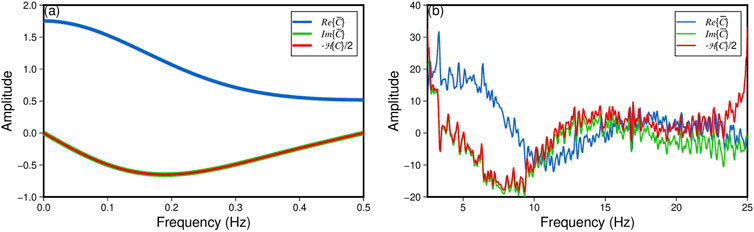
Figure 1. Validation of Equation 9 by comparison of different methods to construct the imaginary part of $\bar{C}(\omega ,r)$: (A) with the input signal described as $\bar{c}(t)={\mathrm{e}}^{-t^2/2}$ for $t>0$, (B) with the input signal as a sample CCF between two virtual stations in a numerical test. Blue lines are the real part of $\bar{C}(\omega ,r)$, which equals $\frac{1}{2}C(\omega ,r)$. Green lines are the imaginary part of $\bar{C}(\omega ,r)$ constructed by the Fourier transform of the causal part of CCFs $(\text{Im}\{\bar{C}(\omega )\})$. Red lines are the imaginary part of $\bar{C}(\omega ,r)$ constructed by the numerical Hilbert transform $-\frac{1}{2}\mathcal{H}[C](\omega )$.

According to Equation 9, the numerical execution of the Hilbert transform can be circumvented in practical scenarios. This is because the Hilbert transform is inherently incorporated during the retention of only the causal portion of the CCFs. Practically, due to the potential asymmetry between the causal and acausal parts of the CCFs, we define the causal part as the average of the positive and negative segments of the CCFs. Additionally, in Luo et al. (2022), only the real part of the integration is used to construct the F-J spectrograms. Therefore, an equivalent expression of the equations used by Luo et al. (2022) would be (see Appendix in Luo et al. (2022)):

$I_{\mathrm{Luo}}\left(\omega ,k\right)=\text{Re}\left\{{\int }_0^{\infty }\bar{C}\left(\omega ,r\right)H_0^{\left(1\right)}\left(kr\right)r\mathrm{d}r\right\},(10)$

$=\frac{1}{2}\text{Re}\left\{{\int }_0^{\infty }\left\{C\left(\omega ,r\right)-\mathrm{i}\mathcal{H}\left[C\right]\left(\omega ,r\right)\right\}{H}_0^{\left(1\right)}\left(kr\right)r\mathrm{d}r\right\}.(11)$

Instead of computing Equation 11 directly, Equation 10 indicates that the numerical Hilbert transform can be avoided in the integration if only the casual part of the CCFs $\bar{C}(\omega ,r)$ is used. Note that in the main text of Luo et al. (2022), $H_0^{(2)}$ in Equations 7, 8, 11, 12 should be replaced by $H_0^{(1)}$. It is also noteworthy that although the usage of Re$\{\cdot \}$ in Equation 10 is not mentioned in Luo et al. (2022), it is required because the corresponding imaginary part of the integrand (denoted by ${I^{*}}_{\text{Luo}}$) fails to correctly constrain the dispersion curves (see details in the Discussion section).

2.4 Comparison among different formulations

In the following section, we summarize other formulations for the improved FJ method with crossed artifacts removed.

Xi et al. (2021) proposed to use

$I_{\text{Xi}}\left(\omega ,k\right)=-{\int }_0^{\infty }\left\{\mathrm{i}G\left(\omega ,r\right)H_0^{\left(2\right)}\left(kr\right)+{\left(\mathrm{i}G\left(\omega ,r\right)\right)}^{*}{H}_0^{\left(1\right)}\left(kr\right)\right\}r\mathrm{d}r,(12)$

where $G$ is the analytic signal defined in Equation 6 and ${(\mathrm{i}G)}^{*}$ is the complex conjugate of $\mathrm{i}G$.

Zhou et al. (2023) proposed to use

$I_{\text{Zhou}}\left(\omega ,r\right)={\int }_0^{\infty }\left[\text{Re}\left\{\tilde{C}\left(r,\omega \right)\right\}{J}_0\left(kr\right)+\text{Im}\left\{\tilde{C}\left(r,\omega \right)\right\}{Y}_0\left(kr\right)\right]r\mathrm{d}r,(13)$

where $\tilde{C}(\omega ,r)$ should be regarded as the analytic signal whose real part is the CCFs $C(\omega ,r)$. Therefore, $\text{Re}\left\{\tilde{C}(\omega ,r)\right\}=C(\omega ,r)$ and $\text{Im}\left\{\tilde{C}(\omega ,r)\right\}=\mathcal{H}[C](\omega ,r)$ according to Equation 3. Note that $\tilde{C}(\omega ,r)\ne G(\omega ,r)$, and Equation 13 seems to be a correct version of Zhou and Chen’s (2021)’s original formulation.

The methods of Xi et al. (2021) and Zhou et al. (2023) have been implemented by Li et al. (2021) for ZZ component CCFs and by Zhang et al. (2022) for multicomponent CCFs. It is important to note, however, that Li et al. (2021) and Zhang et al. (2022) utilized the Python function scipy. fftpack.hilbert in their implementation. This usage has introduced an apparent sign difference when compared to the theoretical analysis presented in this paper.

In a recent study, Yang et al. (2024) proposed the frequency–Hankel transform

$I_{\text{Yang}}\left(\omega ,k\right)={\int }_0^{\infty }\left[\mathcal{H}\left[C\right]\left(\omega ,r\right)+\mathrm{i}C\left(\omega ,r\right)\right]H_0^{\left(1\right)}\left(kr\right)r\mathrm{d}r.(14)$

Combining with the properties of the Hankel function, $H_0^{(1)}(x)=J_0(x)+\mathrm{i}{Y}_0(x)$, $H_0^{(2)}(x)=J_0(x)-\mathrm{i}{Y}_0(x)$, and ${(H_0^1(x))}^{*}=H_0^{(2)}(x)$, formulations presented in Equations 7, 10, 12–14 can be expanded in terms of Bessel functions as

$\begin{array}{ll}\hfill I_{\text{Forbriger}}& ={\int }_0^{\infty }\left[-\mathcal{H}\left[C\right]\left(\omega ,r\right)J_0\left(kr\right)+C\left(\omega ,r\right)Y_0\left(kr\right)\right]r\mathrm{d}r\hfill \\ \hfill & +\mathrm{i}{\int }_0^{\infty }\left[\mathcal{H}\left[C\right]\left(\omega ,r\right)Y_0\left(kr\right)+C\left(\omega ,r\right)J_0\left(kr\right)\right]r\mathrm{d}r,\hfill \end{array}(15)$

$I_{\text{Xi}}=2{\int }_0^{\infty }\left[\mathcal{H}\left[C\right]\left(\omega ,r\right)Y_0\left(kr\right)+C\left(\omega ,r\right)J_0\left(kr\right)\right]r\mathrm{d}r,(16)$

$I_{\text{Luo}}=\frac{1}{2}{\int }_0^{\infty }\left[\mathcal{H}\left[C\right]\left(\omega ,r\right)Y_0\left(kr\right)+C\left(\omega ,r\right)J_0\left(kr\right)\right]r\mathrm{d}r,(17)$

$I_{\text{Zhou}}={\int }_0^{\infty }\left[\mathcal{H}\left[C\right]\left(\omega ,r\right)Y_0\left(kr\right)+C\left(\omega ,r\right)J_0\left(kr\right)\right]r\mathrm{d}r,(18)$

and

$\begin{array}{ll}\hfill I_{\text{Yang}}& ={\int }_0^{\infty }\left[\mathcal{H}\left(C\right)\left(\omega ,r\right)J_0\left(kr\right)-C\left(\omega ,r\right)Y_0\left(kr\right)\right]r\mathrm{d}r\hfill \\ \hfill & +\mathrm{i}{\int }_0^{\infty }\left[\mathcal{H}\left[C\right]\left(\omega ,r\right)Y_0\left(kr\right)+C\left(\omega ,r\right)J_0\left(kr\right)\right]r\mathrm{d}r.\hfill \end{array}(19)$

According to Equations 15–19, there relation is given as

$\text{Im}\left\{I_{\text{Forbriger}}\right\}=\frac{1}{2}{I}_{\text{Xi}}=2I_{\text{Luo}}=I_{\text{Zhou}}=\text{Im}\left\{I_{\text{Yang}}\right\}.(20)$

Denoting the corresponding imaginary part of the integrand in Equation 10 as ${I^{*}}_{\text{Luo}}$, the relation is given as

$\text{Re}\left\{I_{\text{Forbriger}}\right\}=2{I^{*}}_{\text{Luo}}=-\text{Re}\left\{I_{\text{Yang}}\right\}.(21)$

Note that Equation 19 has already been correctly provided by Yang et al. (2024) (Equation 21). However, the construction of $G(\omega ,r)$ in Yang et al. (2024) seems to be problematic (it should be $-a+b\mathrm{i}$ instead of $a+b\mathrm{i}$ on page KS72 in Yang et al. (2024) in their notation according to our Equation 6). The problematic derivation results in their flawed arguments regarding the relationships among different methods.

3 Discussion

As elucidated in Equations 20, 21, the formulations proposed by Forbriger (2003), Xi et al. (2021), Luo et al. (2022), Zhou et al. (2023), and Yang et al. (2024) are actually correlated with each other. Notably, the constructions of $I_{\text{Forbriger}}$, $I_{\text{Xi}}$, $I_{\text{Zhou}}$, and $I_{\text{Yang}}$ all require the numerical computation of the Hilbert transform, as implemented by Li et al. (2021) and Zhang et al. (2022). We would like to emphasize that the numerical Hilbert transform can be avoided in the implementation of $I_{\text{Luo}}$ by merely maintaining the causal portion of the CCFs, or pragmatically, by designating the average of the positive and negative parts of the CCFs as the causal part. To substantiate the efficacy of $I_{\text{Luo}}$, validate the relationship in Equation 20, and study the effects of the real part of $I_{\text{Forbriger}}$ and $I_{\text{Yang}}$, we present a numerical example. In practice, Li et al. (2021) and Zhang et al. (2022) implemented $I_{\text{Xi}}$ and $I_{\text{Zhou}}$ using Equations 16, 18, instead of their original formulations in Equations 12, 13. We, therefore, choose to compare the results of $I_{\text{Luo}}$ and $I_{\text{Xi}}$ using Equations 10, 16 (Figures 2B, C). We also plot ${I^{*}}_{\text{Luo}}$ to study the effects of the real parts of $I_{\text{Forbriger}}$ and $I_{\text{Yang}}$ (Figure 2D). In the numerical example, the seismic arrays are located linearly, as shown in Figure 2B in Luo et al. (2022), and the velocity model contains a low-velocity layer as shown in Figure 2C in Luo et al. (2022). The synthetic waveforms were computed using the Computer Programs in Seismology package (Herrmann, 2013). Subsequently, the vertical–vertical component CCFs were computed. Based on this, the FJ spectrograms of the synthetic data, in accordance with Equations 4, 10, 16, were calculated and illustrated in Figures 2A–C, respectively. In this example, it is clear the crossed artifacts are effectively removed in both Figures 2B, C. Notably, the outputs of $I_{\text{Luo}}$ and $I_{\text{Xi}}$ are almost identical to each other, with the exception that the normalization factor of $I_{\text{Xi}}$ at each frequency is four times that of $I_{\text{Luo}}$, as delineated in Equation 20. On the other hand, the peak locations of the ${I^{*}}_{\text{Luo}}$ spectrogram, corresponding to Re$\{I_{\text{Forbriger}}\}$ and Re$\{I_{\text{Yang}}\}$, do not coincide with the correct dispersion curves (Figure 2D). Therefore, as discussed by Zhou and Chen (2021), the inclusion of Re$\{I_{\text{Forbriger}}\}$ reduces the resolution of FJ spectrograms.

Figure 2

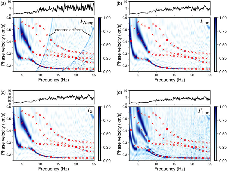
Figure 2. Frequency–Bessel spectrograms of synthetic data computed by the FJ method and three modified versions by Luo et al. (2022) and Xi et al. (2021). (A) FJ spectrogram by integrating with the Bessel function $J_0$ as $I_{\text{Wang}}$ in Equation 4. (B) FJ spectrogram by $I_{\text{Luo}}$ as expressed in Equation 10. (C) FJ spectrogram by $I_{\text{Xi}}$ as expressed in Equation 16. (D) FJ spectrogram by $I_{\text{Luo}}^{*}$, which is the imaginary part of the corresponding integrand in Equation 10. The numerical Hilbert transform was performed to construct $I_{\text{Xi}}$. The theoretical dispersion curves are plotted as red crosses. The normalization factors at each frequency are also plotted at the top of the FJ spectrograms (divided by $10^4$ for visualization).

To further demonstrate the correlations among these methods, we conducted a parallel test using field data from a USArray, as shown in Supplementary Figure S1. The data were previously used in Luo et al. (2022) (see their Figure 9). This test also confirms that both $I_{\text{Luo}}$ and $I_{\text{Xi}}$ are equally effective in removing the crossed artifacts. Additionally, the real part of $I_{\text{Forbriger}}$ should not be included when generating high-resolution FJ spectrograms.

4 Conclusion

In this study, we have conducted analysis of prior work addressing the elimination of crossed artifacts in the frequency–Bessel spectrograms, placing these studies within a unified framework. This approach has allowed us to uncover the underlying relationships between various methodologies proposed in the literature. We also have shown how to extend the formulation proposed by Forbriger (2003) from active to passive sources. Furthermore, we have proposed a refined approach that circumvents the need for the numerical Hilbert transform, as has been implicitly suggested in a previous study (Luo et al., 2022).

Author contributions

XJ: formal analysis, investigation, validation, visualization, and writing–original draft. SH: conceptualization, formal analysis, methodology, validation, and writing–original draft, Writing–review and editing. SL: Software, Writing–review and editing.

Funding

The author(s) declare that financial support was received for the research, authorship, and/or publication of this article. This study was supported by the National Natural Science Foundation of China (42488301, 41904047), Hubei Subsurface Multi-scale Imaging Key Laboratory (China University of Geosciences) (SMIL-2023-8), and the Research and Innovation Initiatives of WHPU.

Acknowledgments

The authors would like to thank the reviewers for their comments that helped them improve the manuscript.

Conflict of interest

The authors declare that the research was conducted in the absence of any commercial or financial relationships that could be construed as a potential conflict of interest.

Generative AI statement

The authors declare that no Generative AI was used in the creation of this manuscript.

Publisher’s note

All claims expressed in this article are solely those of the authors and do not necessarily represent those of their affiliated organizations, or those of the publisher, the editors and the reviewers. Any product that may be evaluated in this article, or claim that may be made by its manufacturer, is not guaranteed or endorsed by the publisher.

Supplementary material

The Supplementary Material for this article can be found online at: https://www.frontiersin.org/articles/10.3389/feart.2025.1505367/full#supplementary-material

References

Erdelyi, A. (1954). Tables of integral transforms, vol. 2, bateman manuscript project. New York, New York: McGraw-Hill.

Google Scholar

Forbriger, T. (2003). Inversion of shallow-seismic wavefields: I. wavefield transformation. Geophys. J. Int. 153, 719–734. doi:10.1046/j.1365-246x.2003.01929.x

CrossRef Full Text | Google Scholar

Hahn, S. L. (1996). Hilbert transforms in signal processing. Boston, London: Artech House.

Google Scholar

Herrmann, R. B. (2013). Computer programs in seismology: an evolving tool for instruction and research. Seismol. Res. Lett. 84, 1081–1088. doi:10.1785/0220110096

CrossRef Full Text | Google Scholar

Hu, B. Y. K. (1989). Kramers–Kronig in two lines. Am. J. Phys. 57, 821. doi:10.1119/1.15901

CrossRef Full Text | Google Scholar

Hu, S., Luo, S., and Yao, H. (2020). The frequency-Bessel spectrograms of multicomponent cross-correlation functions from seismic ambient noise. J. Geophys. Res. Solid Earth 125, e2020JB019630. doi:10.1029/2020JB019630

CrossRef Full Text | Google Scholar

Johnansson, M. (1999). The Hilbert transform. Master’s thesis. Suecia: Växjö University.

Google Scholar

Li, Z., Zhou, J., Wu, G., Wang, J., Zhang, G., Dong, S., et al. (2021). CC-FJpy: a python package for extracting overtone surface-wave dispersion from seismic ambient-noise cross correlation. Seismol. Res. Lett. 92, 3179–3186. doi:10.1785/0220210042

CrossRef Full Text | Google Scholar

Luo, S., Hu, S., Zhou, G., and Yao, H. (2022). Improvement of frequency-Bessel phase-velocity spectra of multicomponent cross-correlation functions from seismic ambient noise. Bull. Seismol. Soc. Am. 112, 2257–2279. doi:10.1785/0120220027

CrossRef Full Text | Google Scholar

Sánchez-Sesma, F. J., and Campillo, M. (2006). Retrieval of the Green’s function from cross correlation: the canonical elastic problem. Bull. Seismol. Soc. Am. 96, 1182–1191. doi:10.1785/0120050181

CrossRef Full Text | Google Scholar

Wang, J., Wu, G., and Chen, X. (2019). Frequency-Bessel transform method for effective imaging of higher-mode Rayleigh dispersion curves from ambient seismic noise data. J. Geophys. Res. Solid Earth 124, 3708–3723. doi:10.1029/2018JB016595

CrossRef Full Text | Google Scholar

Xi, C., Xia, J., Mi, B., Dai, T., Liu, Y., and Ning, L. (2021). Modified frequency-Bessel transform method for dispersion imaging of Rayleigh waves from ambient seismic noise. Geophys. J. Int. 225, 1271–1280. doi:10.1093/gji/ggab008

CrossRef Full Text | Google Scholar

Yang, Z., Sun, Y.-C., Zhang, D., Han, P., and Chen, X. (2024). A frequency-Hankel transform method to extract multimodal Rayleigh wave dispersion spectra from active and passive source surface wave data. Geophysics 89, KS69–KS81. doi:10.1190/geo2023-0189.1

CrossRef Full Text | Google Scholar

Zhang, G., Liu, Q., and Chen, X. (2022). Enhancing the frequency-Bessel spectrogram of ambient noise cross-correlation functions. Bull. Seismol. Soc. Am. 113, 361–377. doi:10.1785/0120220124

CrossRef Full Text | Google Scholar

Zhou, J., and Chen, X. (2021). Removal of crossed artifacts from multimodal dispersion curves with modified frequency-Bessel method. Bull. Seismol. Soc. Am. 112, 143–152. doi:10.1785/0120210012

CrossRef Full Text | Google Scholar

Zhou, J., Li, Z., and Chen, X. (2023). Extending the frequency band of surface wave dispersion curves by combining ambient noise and earthquake data and self-adaptive normalization. J. Geophys. Res. Solid Earth 128, e2022JB026040. doi:10.1029/2022JB026040

CrossRef Full Text | Google Scholar