Reducing dependence of modeled resuspended volcanic ash on meteorological grid resolution

Remobilized volcanic ash from ground deposits can present significant hazards to human health, infrastructure, and aviation. Modeling of ash remobilization events is an important tool that can provide information on the timing and magnitude to assist in planning and response. We investigate how the horizontal resolution of meteorological data, specifically that of friction velocity provided by numerical weather prediction (NWP) models, affects the estimated vertical mass flux and modeled concentrations of volcanic ash. We then apply a method designed to reduce the influence of the resolution on these quantities. Resuspension of volcanic ash from a deposit in Iceland has been modeled with the HYSPLIT atmospheric transport and dispersion model (ATDM) driven by meteorological fields from the European Center for Medium-Range Weather Forecasts (ECMWF) ECMWF Reanalysis v5 (ERA5) dataset and the weather research and forecasting model (WRF) at different resolutions (27 km and 9 km). We tested several simple emission schemes: one widely used for both volcanic ash and dust emissions, one operationally used to forecast ash resuspension in Iceland, and one based on controlled measurements from prepared ash deposits. Scaling factors for emissions were estimated using a cumulative distribution function (CDF) matching technique. Friction velocity values varied significantly across meteorological datasets resulting in considerably different estimates of onsets and vertical mass flux. It is a common approach to compensate for these differences by applying a scaling factor and adjusting the threshold friction velocity. Here, we implement a scheme that utilizes a Weibull distribution for the friction velocity to reduce the dependence of emission estimates on meteorological data resolution. We find that all emission schemes and meteorological datasets can predict the timing of large resuspension events and subsequent transport of the resuspended material. Indeed, the coarser datasets of WRF 27 km and ERA5 perform better than the WRF 9 km in some respects. The use of Weibull distribution for friction velocity successfully reduces the dependence of emission estimates on grid resolution. Similar schemes have been used successfully for dust emissions. Reducing or eliminating this dependence is important in order to assess and compare the success of different emission schemes, threshold friction velocities, and calibration factors.

1 Introduction

For hazard planning purposes, it is important to determine the expected frequency of hazardous conditions and concentrations of ash. Atmospheric transport and dispersion models (ATDMs) are often used to model concentrations of resuspended materials such as volcanic ash and mineral dust. ATDMs require meteorological inputs, such as from a numerical weather prediction (NWP) model, analysis or reanalysis products, or observations. They also require information about the initial position and amount of the material emitted into the atmosphere. To model resuspension with a forward modeling setup, the ATDM requires information about the location of source regions and the mass of the material lifted from each source region as a function of time.

Dust and ash are resuspended by a transfer of momentum from the atmosphere to the deposit. The amount of material resuspended depends on both the state of the atmosphere and properties of the deposit (Kok et al., 2012). Detailed information about deposit properties such as grain size distribution, soil moisture, and deposit depth is not often available. Even the horizontal extent of the deposit may not be clearly known, particularly for fresh deposits of volcanic ash. Furthermore, deposit properties change over time.

An NWP model supplies information about the atmosphere, in particular, the friction velocity that characterizes the momentum flux. However, the spatial and temporal resolutions of the available data may be fairly coarse, and resuspension depends on very local conditions. The modeled mass flux of resuspended material has been shown to be sensitive to the grid resolution of the data (Ridley et al., 2013; Gueye and Jenkins, 2019; Mingari et al., 2017). Vertical mass flux from the surface is related to a high power (generally 3–5) of the friction velocity, and thus, using a mean value for this quantity over an area will provide an underestimation of the true value in case of heterogeneity. Different strategies for reducing the dependence on grid resolution have been developed, including computing emissions on a high-resolution offline grid separately (Meng et al., 2021), estimating emissions from albedo (Chappell et al., 2024), creating a mapping between high- and low-resolution dust emissions (Leung et al., 2023), reducing the threshold friction velocity for coarser resolutions (Klose et al., 2021), and using a distribution for wind speed over the grid square rather than a single value (Ridley et al., 2013; Zhang et al., 2016; Foroutan and Pleim, 2017; Menut, 2018; Tai et al., 2021). Here, we implement a version of the last strategy by utilizing a Weibull distribution for friction velocity.

The processes that govern the resuspension of volcanic ash are generally the same as those for mineral dust and sand, and thus, modeling of resuspended volcanic ash is generally similar to that of dust, but there are important differences (Langmann, 2013; Etyemezian et al., 2019; Del Bello et al., 2021). Fewer studies and measurements of volcanic ash resuspension exist. Measurements conducted by Etyemezian et al. (2019) suggest that fresh volcanic ash deposits can be much more emissive than dust, although they did find that the threshold friction velocities are similar (30–40 cm ${\text{s}}^{-1}$). Particles in ash deposits can be considerably irregularly shaped than dust (Dominguez et al., 2020; Del Bello et al., 2021), which may affect properties such as threshold friction velocities (Del Bello et al., 2021). Here, we focus on modeling the resuspension of ash during large-scale episodic events driven by high wind speeds. These large-scale events pose hazards to human health as well as possible aviation hazards if they occur near airports.

We compare simulated concentrations of resuspended volcanic ash with observations of PM₁₀ at five measurement stations in Iceland. We use an atmospheric transport and dispersion model, HYSPLIT, with three sets of NWP products. The measurements by Leadbetter et al. (2012) are described in Section 2.1. We then describe the modeling setup in which a matrix describing source–receptor relationships is created (Section 2.2). This modeling setup allows for different emission schemes, which are described in Section 2.3, to be applied quickly.

The emission schemes and a technique for reducing dependence on meteorological grid resolution are described in Sections 2.3 and 2.4, respectively. A cumulative distribution function (CDF) matching technique is used to compute calibration or scaling factors for the emission schemes as well as take into account the background (Section 2.5). Evaluation of the different simulations is described in Section 2.6, and results and discussion are presented in Section 3 and Section 4, respectively.

2 Materials and methods

2.1 Measurements

Measurement data are from the Environment Agency of Iceland, and the same measurement data were used in Leadbetter et al. (2012). The data consist of hourly measurements from particulate matter monitors measuring concentrations of particulates less than 10 $\mu$m in diameter (${\text{PM}}_{10}$) at five stations. Resuspended particles less than approximately 20 $\mu$m in diameter can remain in the atmosphere for weeks (Kok et al., 2012).

We focus on the period of 25 May 2010 through 30 June 2010 after the cessation of the eruption of Eyjafjallojökull on 23 May 2010 (Arason et al., 2011). The locations of the measurement sites are shown in Figure 1. Two urban stations, Grensásvegur and Hvaleyrarholt, lie a couple of hundred kilometers to the west and slightly north of the source region. Three stations are located on the edge of the source region, Hvolsvöllur on the east edge, Heimaland to the southeast, and Vík to the south. Measurements of ${\text{PM}}_{10}$ at all the measurement sites are shown in Figure 2. Letters are used to identify resuspension events in which elevated concentrations were observed at one or more of the sites. Seven main resuspension events, A, B, C, D, E, F, and G, were identified. Five smaller events, q, r, s, t, and u, at Hvolsvöllur (Figure 2C) are also discussed. Concentrations at the more distant stations, Hvaleyrarholt and Grensásvegur, were lower in general, remaining below 2,000 $\mu \mathrm{g}{\mathrm{m}}^{-3}$. Concentrations closer to the source sometimes reached above 4,000 $\mu \mathrm{g}{\mathrm{m}}^{-3}$. These values are at least two orders of magnitude higher than background values at the sites and suitable for evaluating our ability to simulate large episodic events most likely driven by higher wind speeds. Visual inspection of the time series at Heimaland, Hvaleyrarholt, and Hvolsvöllur indicates background concentrations on the order of 10 $\mu$g ${\text{m}}^{-3}$. Background values at Grensásvegur are higher, between 10 and 30 $\mu$g ${\text{m}}^{-3}$, and the background values at Vík are approximately 40 $\mu$g ${\text{m}}^{-3}$.

Figure 1

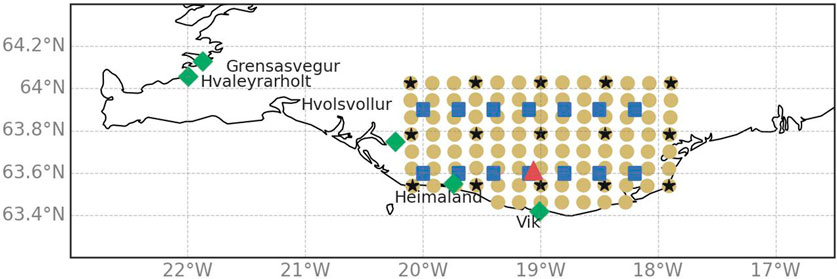
Figure 1. Map of relevant locations in Iceland. Measurements sites are marked as green diamonds. Eyjafjallojökull volcano is shown as the red triangle (${63.61}^o$ N, ${19.06}^o$W). Centers of source locations used for HYSPLIT runs are shown as follows: yellow circles represent grid points from the WRF 9 km dataset, black stars represent grid points from the WRF 27 km dataset, and blue squares represent grid points from the ERA5 dataset.

Figure 2

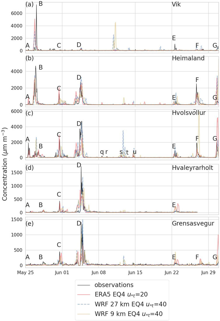
Figure 2. Measured and simulated levels of ${\text{PM}}_{10}$ at each location (a) Vik, (b) Heimaland, (c) Hvollvollur, (d) Hvaleyrarholt, (e) Grensasvegur. Letters on the x-axis (with varying y-axis positions) mark times of elevated ${\text{PM}}_{10}$ levels measured at one or more locations. Emissions were calculated using Equation 4, with $u_{*t}$ = 0.30 m ${\text{s}}^{-1}$ for the ERA5 dataset and 0.40 m ${\text{s}}^{-1}$ for both WRF datasets. Station-specific scaling factors were applied.

2.2 Modeling

HYSPLIT is a Lagrangian transport and dispersion model developed by the National Oceanic and Atmospheric Administration’s Air Resources Laboratory (NOAA ARL) Draxler and Hess (1997), Draxler and Hess (1998); Stein et al. (2015). The model is used operationally at the Washington, Anchorage, Darwin, and Wellington volcanic ash advisory centers (VAACs) for modeling the transport and dispersion of volcanic ash (Beckett et al., 2024) and is also used to model dust resuspension (Draxler et al., 2001; Stein et al., 2010; Ashrafi et al., 2014; Salmabadi et al., 2023). Gridded fields from a meteorological model including the wind field, temperature, humidity, precipitation, and boundary layer height are inputs for the HYSPLIT model. In this study, we use three different meteorological datasets that are described in Section 2.2.1 as model inputs.

2.2.1 NWP modeling

Below, we discuss the meteorological datasets we use in the study and compare with previous studies on regional volcanic ash resuspension that have utilized meteorological fields with various resolutions: 12-km weather research forecasting (WRF) (Folch et al., 2014), 8-km WRF (Mingari et al., 2020), 2-km WRF (Mingari et al., 2017), and a 12-km limited area version of the NWP model from the UK Met Office (Leadbetter et al., 2012; Beckett et al., 2017). These resolutions refer to the horizontal grid spacing of the respective models.

2.2.1.1 ERA5

Data from the European Center for Medium-Range Weather Forecasts (ECMWF) ERA5 global atmospheric reanalysis (Hersbach et al., 2020) were obtained from Copernicus Climate Change and Atmospheric Monitoring Services (2018) and used as input in the HYSPLIT. The dataset has $0.3^o$ latitude–longitude resolution and performs hourly analysis. We used the output on pressure levels, of which there are 37, ranging from 1,000 to 1 hPa. Spacing is 25 hPa between 1,000 and 750 hPa and between 250 and 100 hPa. Spacing is 50 hPa between 750 and 250 hPa. Above 100 hPa, the spacing varies. At high latitude, the grid squares are rectangular, approximately 33 km$\times$14 km. The grid points in the region considered for possible emissions are shown in Figure 1.

2.2.1.2 WRF

The WRF model (Skamarock et al., 2008) version 3.5.1 was run for May through July of 2010 with horizontal resolutions of 27 km (WRF 27 km), 9 km (WRF 9 km), and 3 km (WRF 3 km). In the vertical resolution, there are 34 pressure-sigma levels, with the highest resolution observed near the surface and model top. The upper boundary of the model is at 100 hPa pressure level. The thickness of the lowest layer is approximately 16 m, and there are 20 layers below 850 hPa. The global forecast system (GFS) is used for the model’s initial and outermost lateral boundary conditions. The model is run with the MM5 similarity theory surface layer scheme to compute surface exchange coefficients for heat, moisture, and momentum (Fairall et al., 2003); the Noah land surface model to calculate surface water and energy fluxes (Chen and Dudhia, 2001); the UW planetary boundary layer scheme to compute vertical sub-grid scale fluxes due to eddy transports (Bretherton and Park, 2009); the rapid radiative transfer model for general circulation models (RRTMGs) longwave and shortwave radiation schemes (Iacono et al., 2008); the WRF single-moment 3-class microphysics scheme to predict water vapor, cloud water/ice, and rain/snow concentrations (Hong et al., 2004); and the Grell–Freitas cumulus parameterization to estimate sub-grid-scale updrafts and downdrafts associated with convection and shallow clouds using an ensemble approach that is scale-dependent to allow for a smooth transition as the horizontal resolution increases (Grell and Freitas, 2013). Observational and analysis nudging is employed in the WRF simulations. WRF output fields consist of hourly averages. Since WRF data are on a conformal grid, the grid is close to square. Grid points in the region considered for possible emissions are shown in Figure 1. The 3-km grid points are not shown, but there are nine of them for every 9-km WRF grid point.

2.2.2 HYSPLIT model setup

HYSPLIT model runs were performed, which released one unit of mass for each particle size from every source location every hour from May 22 to 30 June 2010. To reduce the computational time, the runs were only performed for source points in which the friction velocity was greater than 20 cm ${\text{s}}^{-1}$ for WRF 27 km and ERA5 and 30 cm ${\text{s}}^{-1}$ for WRF 9 km, and precipitation was less than 0.01 mm ${\text{h}}^{-1}$ during that hour, as determined from the meteorological dataset. This was done because resuspension is suppressed during precipitation events. We do not investigate the threshold friction velocities below 20 cm ${\text{s}}^{-1}$ as this quantity has generally been measured or calculated to be above the mentioned value (Folch et al., 2014; Beckett et al., 2017; Etyemezian et al., 2019; Mingari et al., 2020; Del Bello et al., 2021).

Sample input files to HYSPLIT are provided in Supplementary Material and provide complete information on the model setup. HYSPLIT was run in the three-dimensional computational particle mode with a variable time step calculated by the model according to the maximum wind speed and grid spacing. Vertical velocities from the meteorological datasets were used to calculate the vertical motion.

As measurements consist of PM₁₀, particle diameters of 1, 5, 10, and 20 $\mu \mathrm{m}$ were modeled. Here, we focus mostly on the 5 $\mu \mathrm{m}$ size. The 1 and 5 $\mu \mathrm{m}$ particles were given a density $2.5\mathrm{g}{\mathrm{c}\mathrm{c}}^{-1}$, while the 20$\mu \mathrm{m}$ particles had a density of $2.2\mathrm{g}{\mathrm{c}\mathrm{c}}^{-1}$ (Bonadonna and Phillips, 2003; Beckett et al., 2016). In HYSPLIT, the particle diameter, density, and shape are used to calculate a settling velocity. Here, the Ganser (1993) and Dare (2015) formulation was used to calculate the settling velocity. All particles were given a shape factor of 1. At an air density of 1.2 kg ${\text{m}}^{-3}$, the settling velocities are $7.6\times 10^{-5}$, $1.9\times 10^{-3}$, $7.6\times 10^{-3}$, and $2.6\times 10^{-2}$ m ${\text{s}}^{-1}$, respectively. As volcanic ash particles are known to have highly irregular shapes, computational particles may be physical particles with a particular fall velocity rather than diameter and density.

The output concentration grid used for each run has a vertical resolution of 50 m and a horizontal resolution of $0.2\times 0.2^o$. A database of friction velocity, precipitation, and 10-m wind speed at each source point at each hour was created from the NWP outputs. Concentrations for each measurement station are extracted from each of the HYSPLIT output files in unit mass per meter cubed. A matrix, T, is constructed, in which the values, $T_{ij}$, are modeled concentrations (in unit mass per volume) for which each source, $i$, contributes to each measurement, $j$. The source is specified by the particle size, location of release, and time of release. Additionally, each source has a friction velocity and 10-m wind speed associated with it. The matrix is then multiplied by an emissions vector, $\vec{E}$, to obtain a modeled concentration vector, $\vec{M}$, with values for the forecast concentrations at each measurement location and time.

$M_j={\displaystyle \sum _i}{E}_i{T}_{ij}.$

The emission vectors are calculated from one of the relationships described in Section 2.3. As discussed previously, Figure 1 shows the center of the source locations, which coincides with the center of the NWP grid cells. The computational particles were released from an area of the size of the grid cell centered on the grid cells.

One advantage of this setup is that once all the model runs are completed, different formulations for determining the emissions can be applied relatively quickly without running the HYSPLIT again. Although many HYSPLIT runs are needed, the individual runs are short, and they can be run in parallel. However, computational time does increase significantly at higher resolution. Here, we only use the WRF 27 km and WRF 9 km resolutions to drive HYSPLIT and leave the use of WRF 3 km for future work. The use of the WRF 3 km resolution for determining emissions is described in Section 2.4.

2.3 Emission estimates

Friction velocity is defined as the product of density and shear stress. The NWP model provides a friction velocity, $u_{\ast }$, which represents the shear stress over or the momentum flux to the surface. In a neutral atmosphere, the relationship between the wind speed and friction velocity is described by the law of the wall.

$u\left(z\right)=\frac{u_{\ast }}{k_v}\mathrm{l}\mathrm{n}\frac{z}{z_0},(1)$

where $u(z)$ is the wind speed at height $z$, $z_0$ is the aerodynamic roughness (the height at which wind speed is 0 m s⁻¹), and $k_v$ is von Karman’s constant $\sim 0.4$. The friction velocity is widely used in emission schemes for resuspended dust and volcanic ash as it represents the transfer of momentum from the atmosphere to the surface.

We consider four simple relationships between emission flux, s, in units of kg ${\text{m}}^{-2}$ ${\text{s}}^{-1}$ and friction velocity in units of m ${\text{s}}^{-1}$.

$s=\left\{\begin{array}{cc}{c}_2{\left(u_{\ast }-u_{*t}\right)}^3\hfill & u_{\ast }\ge u_{*t}\hfill \\ 0\hfill & u_{\ast }<u_{*t}\hfill \end{array}\right..(2)$

Equation 2 is used by Beckett et al. (2017) and Hammond and Beckett (2019) with the factor $c_2=1\times 10^{-3}$ kg ${\text{s}}^2$ ${\text{m}}^{-5}$ computed by the comparison of model output with simulations. The same equation with a different scaling factor is used by Leadbetter et al. (2012). Note that Leadbetter et al. (2012) and Beckett et al. (2017) compute a source strength with units of mass per unit time, which we have converted to a flux by dividing by the approximate area of their emissions, $1\times 10^6$ ${\text{m}}^{-3}$. It is used for daily forecasting of ash resuspension events in Iceland provided by the UK Met Office (Hammond and Beckett, 2019).

$s=\left\{\begin{array}{cc}{c}_3{u}_{\ast }^4\hfill & u_{\ast }\ge u_{*t}\hfill \\ 0\hfill & u_{\ast }<u_{*t}\hfill \end{array}\right..(3)$

Equation 3 was formulated in Westphal et al. (1987) with $c_3=1\times 10^{-5}$ kg ${\text{s}}^3$ ${\text{m}}^{-6}$ and has been used successfully for estimation of ash resuspension since (Folch et al., 2014).

$s=\left\{\begin{array}{c}{c}_4{u}_{\ast }^a\hfill \\ 0\hfill & u_{\ast }<u_{*t}\hfill \end{array}\right..(4)$

Etyemezian et al. (2019) determined $c_4$ and $a$ in Equation 4 by fitting to measurements of $s$ performed at different values of $u_{\ast }$. They provided different estimates of $c_4$ and $a$ for ash sampled from different deposits and different humidity conditions. Here, we use values of a = 5.53 and $c_4=1.349\times 10^{-3}$ kg ${\text{s}}^{4.53}$ ${\text{m}}^{7.53}$, which are the values determined for ash from Mount St. Helens at 50% humidity. For the different ash types and humidities Etyemezian et al. (2019) tested, the exponents ranged from 3.94 to 5.53. As Equation 3 already tests an exponent of 4, and we apply our own scaling as described in Section 2.5, we do not explicitly consider the other relationships in Etyemezian et al. (2019).

$s=\left\{\begin{array}{cc}\frac{k_s{\rho }_{\text{air}}}{g}{u}_{\ast }^3\left(1-{\left(\frac{u_{*t}}{u_{\ast }}\right)}^2\right)\hfill & u_{\ast }>u_{*t}\hfill \\ 0\hfill & u_{\ast }<u_{*t}\hfill \end{array}\right..(5)$

This formulation is from Marticorena and Bergametti (1995) and has been used extensively for dust and ash (Draxler et al., 2001; Folch et al., 2014; Mingari et al., 2020). $k_s$ is a soil texture coefficient, which is set to $5.4\times 10^{-4}$ ${\text{m}}^{-1}$ here (Gillette et al., 1997; Folch et al., 2014). ${\rho }_{\text{air}}$ is the density of air, which is set to 1.225 kg ${\text{m}}^{-3}$ here, and $g$ is the acceleration due to gravity (9.8 m ${\text{s}}^{-2}$).

The above relationships encompass a range of common functional forms of the emission dependence on $u_{\ast }$ and friction velocity, $u_{*t}$. The threshold friction velocity, $u_{*t}$, is the friction velocity below which not enough momentum is available for resuspension to occur. Here and in many simulations, $u_{*t}$ is treated as a constant value. Leadbetter et al. (2012) and Beckett et al. (2017) used 45 and 40 cm ${\text{s}}^{-1}$, respectively.

Etyemezian et al. (2019) measured $u_{*t}$ to be between 0.33 and 0.43 m ${\text{s}}^{-1}$ for a range of relative humidities and ash obtained from two different deposits. Meanwhile, Del Bello et al. (2021) measured $u_{*t}$ between 0.19 and 0.38 m ${\text{s}}^{-1}$ for a deposit in Japan and between 0.13 and 0.19 m ${\text{s}}^{-1}$ for a deposit in Argentina. The low values obtained for the deposit in Argentina were attributed to highly irregular particle shape. Wind tunnel measurements by Del Bello et al. (2018) show that high relative humidity can increase $u_{*t}$ by up to a factor of 2. However, this effect is dependent on properties of the deposit and is non-linear, with significant changes occurring only at high relative humidity levels.

Friction velocity can be more realistically treated as a function of deposit properties. For instance, Folch et al. (2014) and Mingari et al. (2020) implement a scheme in which $u_{*t}$ is a function of particle size distribution of the deposit, soil moisture, and other soil properties. In Mingari et al. (2020), the temporal variation of $u_{\ast }t$ estimated from a relation defined in Fécan et al. (1999) is quite large due to modeled changes in soil moisture, and it varies from less than 40 to up to 80 cm ${\text{s}}^{-1}$. Such an estimation relies on an estimate of the volumetric soil moisture obtained from a meteorological model, which may not be accurate for a fresh volcanic ash deposit, and the maximum amount of water that can be absorbed by the material, $w^{\prime }$, which can vary from approximately 0% for sand to 30% for clay. It is unknown what range of values may be valid for ash, although some studies use a value of 10% (Folch et al., 2014; Mingari et al., 2020).

While we investigate and discuss the effect of changing $u_{*t}$, here, it is treated as a constant within the emission schemes. As noted in Section 2.2, we turn off emissions when precipitation exceeds 0.01 mm ${\text{h}}^{-1}$, which can be interpreted as increasing $u_{*t}$ to a very high value. We would not expect other deposit properties to change significantly during the study period.

2.4 Accounting for horizontal resolution of the NWP model in the emission scheme

It is well known that many dust emission algorithms are dependent on grid resolution (Ridley et al., 2013; Meng et al., 2021; Leung et al., 2023). One way of reducing this dependence is to utilize a distribution for variables such as wind or friction velocity in the equation for emission flux.

$s={\displaystyle \sum _i^N}P\left(u_{*i}\right)F\left(u_{*i}\right)d{u}_{\ast },(6)$

where $F_{u*}$ is a relationship between emission flux and friction velocity, such as described in Equations 2-5. $P(u_{\ast })$ is the distribution of $u_{\ast }$ over the grid square. N and $d{u}_{\ast }$ are chosen appropriately to approximate the integral. Here, we use $d{u}_{\ast }=1$ cm ${\text{s}}^{-1}$. The Weibull distribution given by Equation 7 is often used for wind speed and has been used for momentum flux as well (Ridley et al., 2013; Klose et al., 2014; Zhang et al., 2016; Menut, 2018; Tai et al., 2021).

$P\left(u_{\ast };k,\lambda \right)=\left\{\begin{array}{cc}\frac{k}{\lambda }\left({\frac{u_{\ast }}{\lambda }}^{k-1}\right)e^{-{\left(x/\lambda \right)}^k}\hfill & u_{\ast }>u_{*t}\hfill \\ 0\hfill & u_{\ast }<u_{*t}\hfill \end{array}\right.,(7)$

$k={\left(\frac{{\bar{u}}_{\ast }}{{\sigma }_{u_{*}}}\right)}^{1.086},(8)$

$\lambda =\frac{{\bar{u}}_{\ast }}{\mathrm{\Gamma }\left(1+1/k\right)},(9)$

where $k$ and $\lambda$ are the shape and scale parameters of the distribution, respectively. The goal is to use only information from the coarse dataset to estimate emissions using Equations 6 and 7. To do this, we take friction velocity from the coarse dataset, $u_{*c}$, as an adequate approximation to ${\bar{u}}_{*}$ in Equation 8. The variability in friction velocity in the WRF 3-km dataset is then used to estimate the relationship given in Equation 10 between $u_{*c}$ and ${\sigma }_{u_{*}}$, as described below. Finally, $k$ and $\lambda$ are calculated from the $u_{*c}\approx {\bar{u}}_{\ast }$ using Equations 8–10.

For each grid box in the WRF 27 km dataset, there are 81 values from the WRF 3 km, and similarly for the WRF 9-km dataset, there are nine values. Figure 3a shows the standard deviation of the friction velocities in the fine resolution WRF 3-km dataset, ${\sigma }_{u_{*}}$, versus the friction velocity of the coarse dataset WRF 27 km, $u_{*c}$. The relationship between $u_{*c}$ and ${\sigma }_{u_{*}}$ can be approximated by a linear fit to the data, as given in Equation 10.

Figure 3

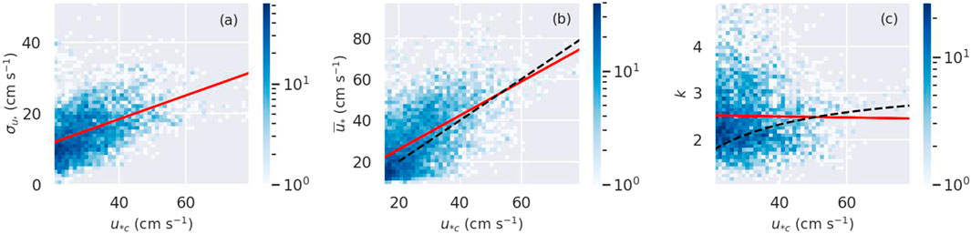
Figure 3. (a) Histogram of standard deviation of the WRF 3 km friction velocities vs. the friction velocity of the WRF 27 km. The red line is a linear fit to the data (Equation 10). The slope is 0.332 with standard error 0.009, the intercept is 5.13 with standard error 0.31, and the Pearson correlation coefficient (PCC) = 0.456. (b) Histogram of the mean of the WRF 3 km friction velocities vs. friction velocity of the WRF 27 km. The red line is a linear fit to the data with slope 0.822 and standard error 0.015; the intercept is 9.5 with standard error 0.4, and PCC = 0.56. The black dotted line is the 1:1 line. (c) Histogram of the shape parameter calculated from each fit of a Weibull distribution to the 81 WRF 3 km friction velocities at each location and hour. The red line is a linear fit to the points with slope of −0.001 with standard error 0.001, intercept of 2.53 with standard error of 0.04, and PCC = −0.01. The black line is $k$ calculated using the fit to the standard deviation given in Equation 10 and Equation 8. Color bars show the number of counts in each bin, and the color is on a log scale. The linear fits are calculated with the Python SciPy module (Virtanen et al., 2020) linregress function. The function returns a slope, intercept, PCC, and standard error for the slope and intercept.

The same process is followed for the WRF 9 km and ERA5 datasets, as shown in the Supplementary Material. The relationship between $u_{*c}$ and ${\sigma }_{u_{*}}$ for the ERA5 is close enough to that found for the WRF 27 km dataset that we simply use the same relationship for both.

${\sigma }_{u_{*}}\approx \left\{\begin{array}{cc}0.332u_{*c}+5.13\hfill & \mathrm{W}\mathrm{R}\mathrm{F}27\mathrm{k}\mathrm{m}\hfill \\ 0.206u_{*c}+1.72\hfill & \mathrm{W}\mathrm{R}\mathrm{F}9\mathrm{k}\mathrm{m}\hfill \end{array}\right..(10)$

Figure 3b shows the histogram of the mean of the 81 WRF 3-km friction velocities vs. the friction velocity of the WRF 27 km, which we use to check our assumption that $u_{*c}\approx {\bar{u}}_{\ast }$. Although there is a lot of scatter, a linear fit is close to the 1:1 line, and the two quantities are correlated. This indicates that the value of $u_{\ast }$ in the coarse grid is an acceptable approximation to the mean.

Figure 3c shows the histogram of shape parameters obtained from fitting a Weibull distribution to the WRF 3 km data vs. $u_{*c}$ and provides comparison to $k$ calculated from Equations 10, 8. The fits to the WRF 3-km data were performed with the Python SciPy module (Virtanen et al., 2020) using the weibull_min.fit function. The red line shows a linear fit to the points making up the histogram, while the black dotted line shows k values computed from $u_{*c}$ and Equations 8, 10. Using these equations produces shape parameters between approximately 1.8 and 2.7 for $u_{\ast }$ between 20 and 80 cm ${\text{s}}^{-1}$ for WRF 27 km, which roughly agrees with the results from fitting a Weibull distribution to the WRF 3 km data.

Following the same procedure for the WRF 9 km data produces shape parameters between approximately 4 and 5 for $u_{\ast }$ between 20 and 140 cm ${\text{s}}^{-1}$, which also agrees with results from the fitting.

Larger values of the shape parameter indicate a distribution with a narrower peak, so it makes sense that the shape parameter value will increase as the grid resolution becomes finer, and there is less variation in $u_{\ast }$ over the grid square (Menut, 2018). The shape parameter value is also lower for lower friction velocity, which usually correspond to lower wind speeds, which tend to have more variability.

Figure 4 shows examples of Weibull distributions for a time period for the 15 WRF 27- km source locations. As seen from the large scatter in Figure 3a, $u_{*c}$ is often different from the mean of the sub-grid values. At this particular time period, $u_{*c}$ is often smaller than ${\bar{u}}_{\ast }$. There may be ways to reduce the scatter in the relationship between the two, which can be investigated in future work.

Figure 4

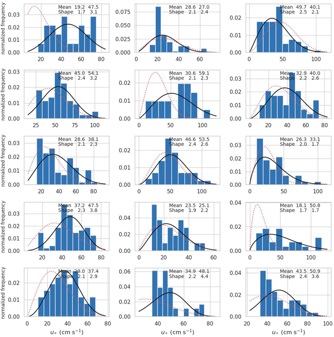
Figure 4. Each plot represents one source location in the WRF 27 km dataset and the source points in the WRF 3 km dataset which are within the WRF 27 km grid square on 01 June 2010 the time 00:00 UTC. The blue bars are the normalized histogram of WRF 3 km friction velocities. The black line is a Weibull distribution fit to the histogram. The red dotted line is a Weibull distribution computed from the friction velocity of the WRF 27 km dataset being used as an approximation for the mean and Equations 10, 8 to calculate the shape, $k$. The mean and shape of the distributions are given in the top right corner, with the first set of numbers belonging to the red dotted curve and the second set belonging to the solid black curve.

Figure 4 also illustrates the uncertainty in estimating the distribution and parameters from a relatively small sample size. To check the suitability of the Weibull distribution, we used a fitting program called distfit (Taskesen, 2020) to rank how well 10 different distributions fit the data according to the residual sum of squares (RSS) and found that Weibull performed the best overall (see Supplementary Material).

Our method here differs from similar work mainly in two respects. First, it uses a distribution for $u_{\ast }$ rather than wind speed. Second, it looks at regional transport of volcanic ash and uses generally higher-resolution datasets, while most previous studies focus on the global transport of dust. Ridley et al. (2013) used GEOS-Chem at $4^o\times 5^o$ and $2^o\times 2.5^o$ resolution with higher-resolution winds at $0.25^o\times 0.3125^o$ resolution to calculate the shape parameter of the Weibull functions. Zhang et al. (2016) used CAM5 at $1.9^o\times 2.5^o$ horizontal resolution to study global dust emissions. A 15-km ECMWF analysis and some regional WRF 3-km runs are used for comparison. Tai et al. (2021) used the GEOS-Chem global chemical transport model on a $2^o\times 2.5^o$ resolution grid and the MERRA reanalysis dataset at $0.333^o\times 0.666^o$ resolution for downscaling. Menut (2018) used WRF and CHIMERE with 60-km resolution. They do not use a finer grid resolution to estimate the shape parameter but instead rely on a relationship between the shape parameter and the mean velocity.

2.5 Computing the scaling factor

It is a generally accepted practice to compute a scaling or calibration factor for the emission scheme by comparing simulated concentrations with observations, although the methods to do so vary (Leadbetter et al., 2012; Folch et al., 2014; Beckett et al., 2017; Mingari et al., 2020).

To compute the scaling factors, $\varphi$, we use cumulative distribution function, CDF, and matching (Reichle and Koster, 2004; Piani et al., 2010; Gudmundsson L. et al., 2012; Belitz and Stackelberg, 2021; Crawford et al., 2022), which transforms forecast values so that their CDF more closely matches that of the observations. Figure 5 shows an example of the CDF matching at two measurement sites. The modeled and observed values are sorted from greatest to least and then paired. A linear fit is applied to the difference between the pairs as a function of the forecast value, as shown in Figures 5a, b. Then, the forecast values are transformed according to Equation 11.

$c^{\prime }=\left(1-\varphi \right)c-\alpha ,(11)$

where $c$ is the original value and $c^{\prime }$ is the transformed value. $1-\varphi$ and $\alpha$ are the slope and intercept of the fit, respectively. Figures 5c, d compare the CDF of the observations, the original forecast values, and the transformed values. Figures 5e, f compare the time series of observations and transformed values, respectively. The technique reduces bias by transforming the forecast, so the area of the forecast time series curve above the observations matches the area below it. One advantage of this method is that it is not affected by incorrect predictions of the timing of the peaks.

Figure 5

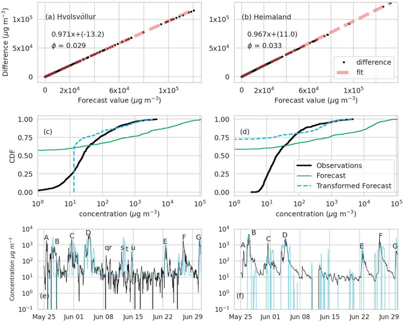
Figure 5. Examples of the CDF matching procedure at two stations, Hvolsvöllur (a, c, and e) and Heimaland (b, d, and f). The examples use the 27 km WRF dataset and Equation 3 for emissions with $u_{*t}=0.4$ m ${\text{s}}^{-1}$. Figures (a) and (b) show the linear fit to the differences between the paired data. Figures (c) and (d) show the CDF for the observations, forecast CDF, and transformed forecast CDF. Figures (e) and (f) show the transformed modeled concentrations (thick cyan line) compared with the observations (thin black line). Note that in (f), modeled values that were previously 0 were shifted to −11.6 and are not shown due to the log scale.

The intercept can be interpreted as the background value of the observations when it is negative. The intercept only correctly represents the background when the forecast correctly captures the magnitude, duration, and number of peaks. If the simulation over-forecasts the peaks, then the background value will be shifted lower or even to a negative value (positive intercept), which is not physical. If the simulation under-forecasts the peaks, then the background value will be shifted higher.

Figures 5a, c, e show a case when the intercept is negative, which is most often the case. Figures 5b, d, f show a case when the intercept is positive. Subtracting the positive intercept then leads to negative concentrations at some times, which is not physical. An additional step could be taken to then adjust those to 0.

Here, we calculate $\varphi$ for each observation site and use the median of those values for calculating the total mass resuspended. This allows for different background values at the different sites. An alternative method is to subtract the background estimated at each site from the observations and then calculate the scaling factor using CDF matching on the whole dataset. However, we found that in cases where the scaling factors could be quite different, this was too sensitive to the outliers.

2.6 Evaluation

We compute statistics, root-mean-square error (RMSE), and Pearson correlation coefficient (PCC) using the forecasts adjusted individually at each station. We do not report a traditional measure of bias because it is near zero in all cases due to the use of CDF matching. This method of computing the statistics gives a best-case scenario.

We provide the ratio of the highest scaling factor to the lowest and indicate it by $\alpha$. If $\alpha$ is 1, that means that the scaling factor computed at all stations was the same. The larger $\alpha$ is, the larger the bias (as well as RMSE) would be if using simulated values calculated with only one scaling value for the emissions. As discussed in Section 2.5, bias can also be inferred from values of the intercept that are not reasonable background values. For instance, a positive intercept indicates high bias, while a negative intercept that is larger than a reasonable background value indicates low bias. The total amount of the material emitted is calculated using the median scaling factor ${\varphi }_m$.

3 Results

3.1 Emission estimates and friction velocity

Figure 6 shows the joint histograms of friction velocity and 10 m wind speed, as well as the relationship between $u_{\ast }$ and wind speed given by Equation 1 for different $z_o$. In the WRF datasets, the highest friction velocities are not associated with the highest wind speeds, but rather with higher roughness values. Additionally, in the ERA5 dataset, $z_o$ is between 0.05 and 5 cm, while in the WRF datasets, it is between 0.05 and 50 cm.

Figure 6

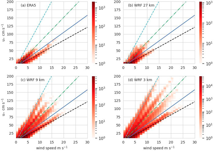
Figure 6. Two-dimensional histograms of $u^{\ast }$ and wind speed for all source points for (a) ERA5, (b) WRF 27 km, (c) WRF 9 km, (d) WRF 3 km. The solid lines show Equation 1 with $z_o$ = 0.05 cm (black dashed line on the right), 5 cm (blue solid line), 10 cm (green dash-dot line), and 50 cm (cyan dashed line on the far left).

The time series of $u_{\ast }$ values for the different datasets show very similar temporal variation, with peak values generally coinciding with identified emission episodes (Supplementary Figure S9 in Supplementary Material). However, the peak values are quite different with values between 40 and 70 cm ${\text{s}}^{-1}$ for ERA5, 50 and 80 cm ${\text{s}}^{-1}$ for WRF 27 km, and 80 and 140 cm ${\text{s}}^{-1}$ for WRF 9 km. Given the power law relationship between $u_{\ast }$ and emission flux, this naturally leads to emission estimates that have similar temporal variation but quite different strengths, as shown in Figure 7. This figure also shows the effect of using a Weibull distribution for $u_{\ast }$. Peak values of emissions tend to increase significantly and are in better agreement with the 3-km WRF. The range of emission values also increases because when $u_{\ast }<u_{*t}$, the portion of the distribution above $u_{\ast }$ still produces some emissions. This leads to better agreement with the 3-km WRF during the time periods of low emissions as well.

Figure 7

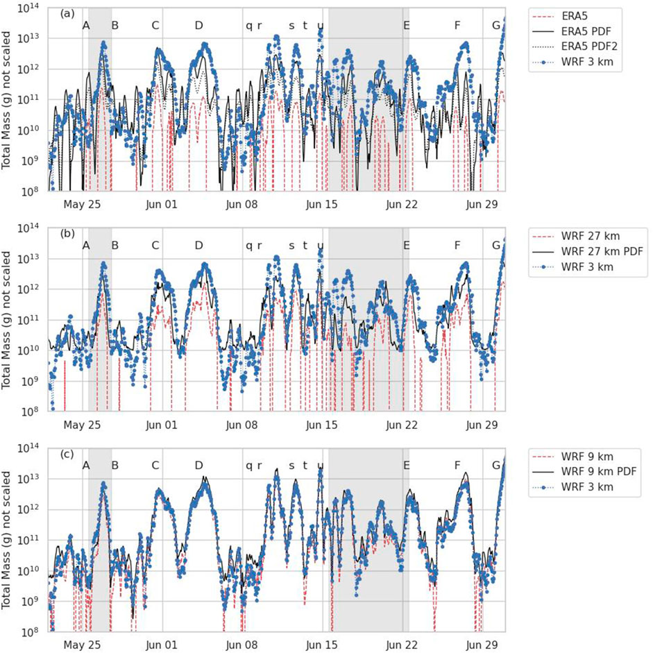
Figure 7. Time series of the total mass resuspended as predicted by Equation 4 with $u_{*t}=30$ cm ${\text{s}}^{-1}$. Each plot shows emissions calculated using $u_{\ast }$ from the WRF 3 km dataset in blue circles and dotted lines. The other lines indicate emissions calculated as indicated. (a) ERA5 using $u_{\ast }$ and Weibull distribution for $u_{\ast }$ with shape parameter k = 1.5 (dark black line) and shape from Equations 8, 10 (dotted black line). (b) WRF 27 km using $u_{\ast }$ and Weibull distribution for $u_{\ast }$ using shape from Equations 8, 10. (c) WRF 9 km data using $u_{\ast }$ and Weibull distribution using shape from Equation 10. The shaded area marks periods when emissions are noticeably suppressed by precipitation, as shown in Figure 8.

The WRF 9 km and WRF 3 km data already agree fairly well, especially at the peaks, even without using a PDF for $u_{\ast }$, indicating that the 9 km horizontal resolution may be sufficient for this time period and area.

Figure 8 is the same as Figure 7, except sources with precipitation greater than 0.01 mm ${\text{h}}^{-1}$ have been removed. As may be expected, accounting for precipitation has a large effect. Emissions are suppressed significantly during a couple of time periods, which are indicated by the shaded regions.

Figure 8

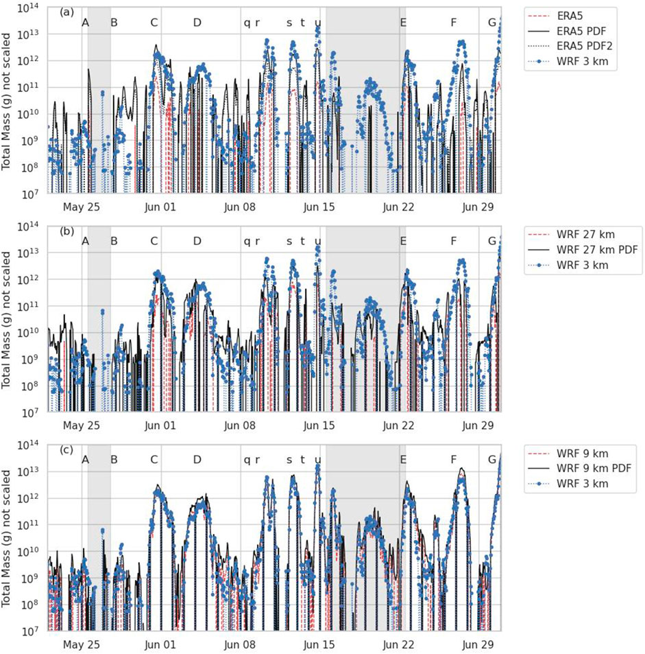
Figure 8. Same as Figure 7, except sources with precipitation greater than 0.01 mm ${\text{h}}^{-1}$ have been removed. (a) ERA5 compared to WRF 3 km, (b) WRF 27 km compared to WRF 3 km, (c) WRF 9 km compared to WRF 3 km. The shaded area marks periods when emissions are noticeably suppressed by precipitation, as compared with Figure 7.

3.2 Modeled concentrations

Figure 2 shows modeled concentrations compared to observations at all five measurement sites. An example using each meteorological dataset is shown. Changing the emission scheme or threshold friction velocity tends to only change the magnitudes of the peaks somewhat. Qualitatively, episodes A, B, and C seem to be captured best by ERA5.

Episode A is predicted only by ERA5. Episode B is predicted at Vík by ERA5 and WRF 27 km, with the simulated arrival time being approximately 9 h too early. At Heimaland and Hvolsvöllur, all three datasets predict episode B, with the WRF datasets showing the peak to be large and sharp at Hvolsvöllur and ERA5 being closer.

Episode D is captured fairly well by all three meteorological datasets, with the WRF 27 km arguably reproducing the timing and duration of the peak the best.

At higher $u_{*t}$ thresholds that do not utilize the PDF, these peaks are not seen. The WRF 9-km dataset also performs fairly well for q through u at Hvolsvöllur, but it does produce peaks during this time period at the other sites as well. In particular, the main reason for the poor performance of WRF 9 km at Vík is a large peak that occurs between episodes r and s. The WRF 27 km produces peaks that are too large as well as peaks at the other sites.

Episode E is quite mixed. The WRF 27 km seems to perform the best. It shows a small peak at approximately 100 $\mu$g ${\text{m}}^{-3}$ around episode E at Vík, which is hard to see on the linear scale plot. It slightly overestimates concentrations at Heimaland, but it gets both the magnitude and timing correct at Hvolsvöllur, Hvaleyrarholt, and Grensásvegur. ERA5 and WRF 9 km datasets also show peaks for episode E at all stations, except Vík, but the timing and/or magnitudes are not quite in agreement.

Figure 9 provides the values described in Section 2.6 for the three meteorological datasets using different emission schemes and $u_{*t}$. Figure 10 is the same but uses distributions for $u_{\ast }$ as in Equation 6.

Figure 9

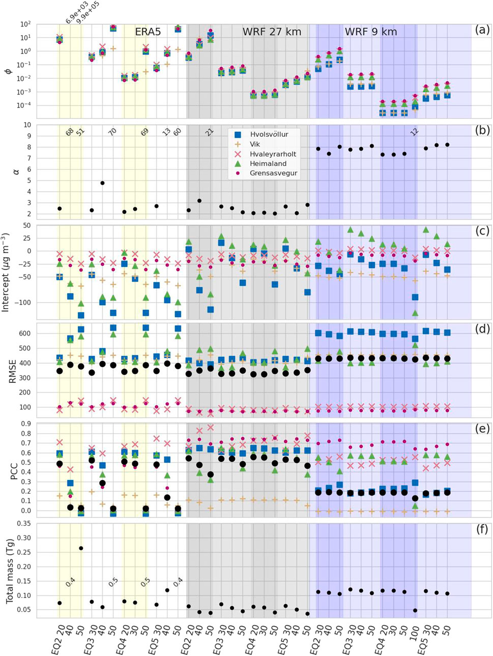
Figure 9. (A) Scaling factor, $\varphi$, determined from CDF matching. If values are above 100, the median value is written as text at the top. (B) Ratio, $\alpha$, of the highest to lowest scaling factor. If the value is above 10, it is written as text near the top. (C) Intercept from CDF matching. Negative intercept can be interpreted as an estimated background value. (D) RMSE of simulation data corrected with CDF matching. (E) Pearson correlation coefficient of simulated concentrations corrected with CDF matching. (F) Total mass emitted in simulation using the median scaling factor from all five stations. Values above 0.150 are written in text near the top. The label on the bottom indicates which equation was used to calculate emissions and $u_{*t}$ in cm ${\text{s}}^{-1}$. The white/yellow area is simulations driven with the ERA5 dataset, the gray area is for simulations driven with the WRF 27 km dataset, and the blue area is for simulations driven with the WRF 9 km dataset. The shaded regions separate different emission schemes.

Figure 10

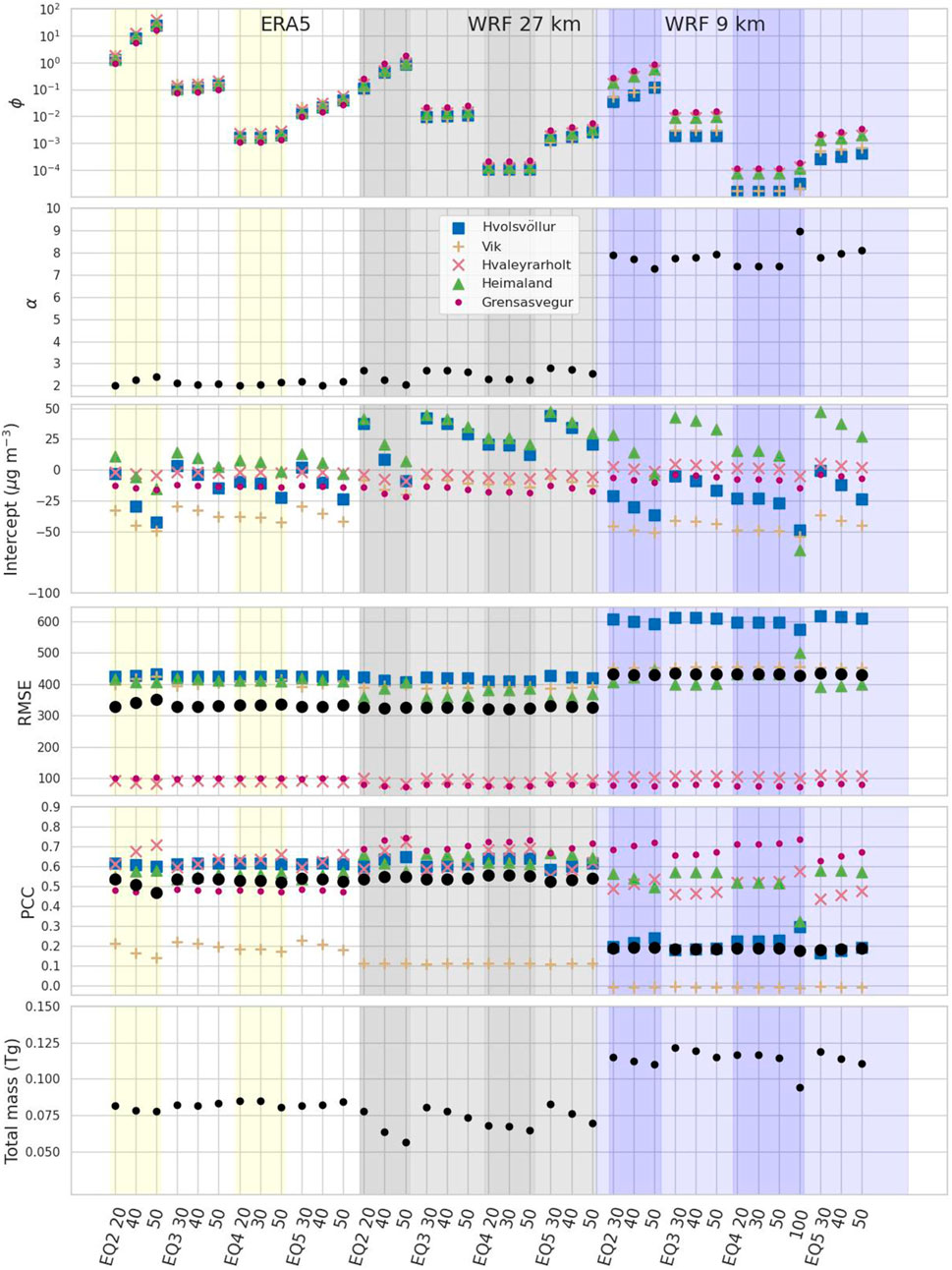
Figure 10. Same as Figure 9, except emissions were calculated with a Weibull distribution for $u_{\ast }$, as described in Section 2.4. The same distribution was used for the ERA5 and WRF 27 km datasets.

The three different meteorological datasets are shown in the order from the most coarse on the left to the least coarse on the right. Results for the different functional forms are shown with different values of $u_{*t}$ increasing from left to right. All results are for utilizing only the $5\mu \mathrm{m}$ diameter particle size. A discussion of how changing the particle size affects the results is provided in the following text.

Simulations using the WRF 27 km and ERA5 data produced the lowest values of $\alpha$, while simulations using WRF 9 km data produced the highest values of $\alpha$. For the 9 km WRF, Hvolsvöllur consistently had the lowest $\varphi$, followed by Vík, Hvaleyrarholt, Heimaland, and Grensásvegur. For the 27-km WRF, Hvaleyrarholt and Grensásvegur tended to have the largest scaling factor. Higher scaling factors being estimated at the more distal stations indicates a possible problem with transport processes, which could be related to deposition, vertical mixing, and errors in mean winds. Folch et al. (2014) also found that simulated concentrations are underestimated at stations far from emission points and overestimated at closer stations.

Given a meteorological dataset, scaling factors were lowest for Equation 4 and highest for Equation 2. This may be expected as the scaling in Equation 2 was already computed with a similar method as given here, while Equation 4 is from point measurements of prepared bare ash samples. And thus, the scaling factor must account for adjustments such as drag partition (King et al., 2005).

The scaling factor tends to increase as $u_{*t}$ is increased. As might be expected, this relationship is more pronounced for Equations 2, 5, in which the excess friction velocity $u_{*}-u_{*t}$ is utilized. It is also more pronounced when the distribution is not used for $u_{\ast }$ and in meteorological datasets in which the range of $u_{\ast }$ is smaller.

Figure 11 compares the scaled emission flux as a function of $u_{\ast }$ for the different emission schemes, threshold friction velocities, meteorological inputs, and use of distribution for $u_{\ast }$. The similarities between the emission fluxes for the same meteorological inputs help explain why the performance is quite similar for the different emission schemes. It is also evident why the estimates using WRF inputs, particularly the WRF 9 km, are insensitive to changes in the $u_{*t}$. For WRF 9 km, the emission fluxes cover almost three orders of magnitude between $u_{\ast }=40$ and 140 cm ${\text{s}}^{-1}$. The higher emissions dominate for the events that we are evaluating, and it does not matter much if the lower emissions are included or not. The measurements we are using are not sensitive to the low emissions. For the WRF 9 km data, results using $u_{*t}=30$ through 50 cm ${\text{s}}^{-1}$ are almost identical, and real differences are not seen until $u_{*t}$ close to 100 cm ${\text{s}}^{-1}$ is used, at which point simulation performance degrades.

Figure 11

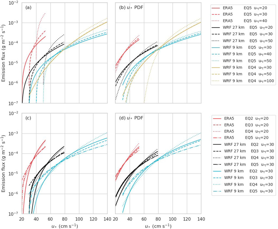
Figure 11. Scaled emission flux as a function of friction velocity. The median scaling factor from all five measurement sites was used. Figures (a) and (b) show the effect of changing $u_{*t}$. Figures (c) and (d) show the effect of changing the functional form of the relationship between $s$ and $u_{\ast }$. Figures (b) and (d) use a Weibull distribution for $u_{\ast }$ with shape,$k$, calculated from Equations 10 and 8. The ERA5 uses the same equations as WRF 27 km dataset.

On the other hand, estimates using ERA5 are quite sensitive to $u_{*t}$ due to the reduced range of $u_{\ast }$ values. Reducing the $u_{*t}$ value as in Klose et al. (2021) can be a valid strategy for coarser datasets. However, using the distribution for $u_{\ast }$ may be preferable.

The total mass suspended was estimated to be approximately 0.075 Tg for ERA5, between 0.05 TG and 0.075 TG for WRF 27 km, and approximately 0.11 Tg for WRF 9 km. The different scaling factors tend to preserve the total mass resuspended. According to Gudmundsson et al. (2012), the total amount of airborne tephra produced by the eruption was $270\times 10^6{m}^3$, with $140\times 10^6{m}^3$ (density of 1,400 kg ${\text{m}}^{-3}$) depositing in Iceland. The deposit amounts would thus amount to approximately 200 TG.

Given an emission equation, scaling factors were highest for ERA5 and lowest for WRF 9 km. This is related to the range of $u_{\ast }$ values in the datasets that are lowest for ERA5 and highest for WRF 9 km. Using a Weibull distribution for $u_{\ast }$ decreased this difference in scaling factors across the different meteorological datasets significantly. The scaling factors for WRF 9 km and WRF 27 km went from being close to an order of magnitude different to being on order of the same magnitude for the Grensásvegur, Heimaland, and Hvolsvöllur stations.

Figures 12, 13 illustrate the effect of using the distribution for $u_{\ast }$ on the time series of concentrations. These figures are similar to Figure 2 but are shown on a log scale. Figure 12 compares results using ERA5 and Equation 4. Comparison of the red and blue line shows the effect of increasing the friction velocity threshold without using a distribution. Meanwhile, comparison of the red and yellow line shows how using a distribution has a similar effect as lowering $u_{*t}$, which is a strategy used in Klose et al. (2021). Notably, the red and yellow lines are similar despite having very different threshold friction velocities. For example, episodes q through u, which only show peaks at Hvolsvöllur, are best represented by the ERA5 with a lower $u_{*t}$ of 20 cm ${\text{s}}^{-1}$ or a $u_{\ast }$ PDF.

Figure 12

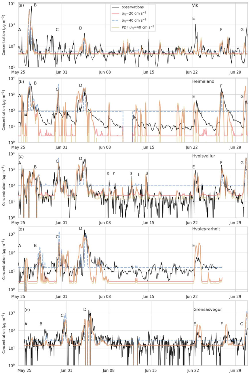
Figure 12. Measured and simulated levels of ${\text{PM}}_{10}$ at each location (a) Vik, (b) Heimaland, (c) Hvollvollur, (d) Hvaleyrarholt, (e) Grensasvegur. Letters are placed at the same location on the x-axis (y-axis location may differ) to indicate times at which elevated ${\text{PM}}_{10}$ levels were measured at one or more locations. Equation 4 was used to calculate emissions with the ERA5 dataset. Threshold friction velocities are as indicated in the legend. The yellow lines are results using a Weibull distribution for $u_{\ast }$, as indicated by PDF in the legend. The scaling factors and background computed for each individual station were used.

Figure 13

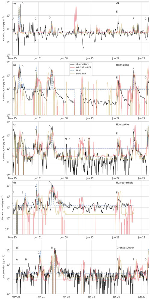
Figure 13. Measured and simulated levels of ${\text{PM}}_{10}$ at each location (a) Vik, (b) Heimaland, (c) Hvollvollur, (d) Hvaleyrarholt, (e) Grensasvegur. Letters are placed at the same location on the x-axis (y-axis location may differ) to indicate times at which elevated ${\text{PM}}_{10}$ levels were measured at one or more locations. Equation 4 was used to calculate emissions with $u_{*t}$ = 40 cm ${\text{s}}^{-1}$. The red line shows ERA5 using no distribution. The blue dashed line shows ERA5 using a distribution for $u_{\ast }$. The yellow line shows WRF 9 km using a distribution for $u_{\ast }$. The scaling factors and background computed for each individual station were used.

However, using the distribution has advantages over simply reducing $u_{*t}$, such as it also reduces the difference between the scaling factors. Because of the scaling factors, the magnitude of the peaks in the plots remains very similar, and differences are difficult to see on a linear scale plot. Using a log scale as shown here, the most noticeable differences are the changes in the estimated background value (intercept from the CDF matching), number of small peaks, and width of the peaks. Because the range of $u_{\ast }$ in ERA5 is fairly small, the modest increase in $u_{*t}$ reduces the number of small peaks and width of peaks. Figure 13 is almost the same as 12, except the red line is now the WRF 9 km with the same $u_{*t}=40{\mathrm{c}\mathrm{m}}^{-1}$ as the other two lines and using a distribution for $u_{\ast }$. The main point here is that if the distribution is used for $u_{\ast }$, the results from using ERA5 and WRF 9 km are much more similar (yellow and red lines). When the distribution for $u_{\ast }$ is not used, then, ERA5 produces much narrower and fewer peaks than the WRF 9 km dataset with the same $u_{*t}$ (yellow and blue lines). Additionally, the scaling factors are much farther apart.

As shown in Figure 10, the only relationship that produces scaling factors near 1 is Equation 2. A scaling factor near 1 indicates agreement with the scaling factor determined by Beckett et al. (2017). Folch et al. (2014) determined a scaling factor of 0.1 for Equation 3, which is similar to what we see for ERA5 with the Weibull distribution for $u_{\ast }$ (Figure 10) and for the WRF 27 km without the distribution (Figure 9).

Negative values of intercept from the CDF matching that agree with the background indicate that the model is correctly capturing the amount of mass in the peaks. Positive values of the intercept from the CDF matching indicate a high bias or over-forecasting of peaks. We see this only at the Heimaland station for most of the WRF 9-km runs and a few of the WRF 27-km runs. We also see large negative values of the intercept occurring particularly when $u_{*t}$ is too large. This occurs because some peaks have been reduced or even eliminated entirely, leading the simulation to under-forecast the peaks. The CDF matching makes up for this by adding a larger value.

RMSE is significantly lower at the two distal stations, Grensásvegur and Hvaleyrarholt. It is similar across all simulations, with the exception that the RMSE for Hvolsvöllur for the WRF 9 km dataset is significantly higher. PCC also decreases significantly, and visual inspection confirms that peaks produced by the WRF 9 km dataset at this station tend to be offset slightly in time. Overall, the WRF 27 km dataset also produces simulations with the highest PCC.

Arguably, the most important performance metric shown here is $\alpha$. A value near 1 would indicate that emission fluxes estimated from all observation sites were in agreement. However, the lowest value of $\alpha$ achieved was 2 through simulations with both ERA5 and WRF 27 km datasets. The simulations using WRF 9 km produced $\alpha$ of 7–8, which is quite high and seems to be driven mostly by a couple of large misplaced peaks predicted at Vík and Hvolsvöllur, which drive $\varphi$ lower and cause lower values for PCC and higher values for RMSE.

We looked at the effect of using different particle sizes along with the Weibull distribution by repeating the analysis carried out so far with different particle sizes in place of the 5 $\mu$m particles. As the simple emission schemes we use do not contain any terms dependent on particle size, any differences are due to transport and deposition. The large particle sizes will tend to remain lower in the atmosphere and deposit faster due to increased gravitational settling. Reducing the particle size used to 0.1 $\mu$m diameter had very little effect on any of the results. Increasing the particle size to 20 $\mu$m did affect the results. It decreased $\alpha$ slightly in the WRF 9 km simulations to approximately 6 or 7, but it also increased alpha in the ERA5 and WRF 27 km simulations to approximately 5. Those increases were driven by a larger increase in $\varphi$ for the distal stations than for the closer stations, which is probably due to increased settling and deposition of the larger particles. The pattern and magnitude of the peaks with the scaling applied remained the same, with some variations in values. The same trends were seen in the 10 $\mu$m particle size to a lesser extent. For the WRF 27-km simulations, $\alpha$ was increased slightly to approximately 3. Plots similar to Figure 10 for the different particle sizes can be found in Supplementary Material.

4 Discussion

This investigation mainly focused on reducing differences in estimated emissions due to differences in meteorological grid size. Utilizing methods to account for meteorological grid resolution has several advantages. It should allow for better agreement in scaling factors and optimal threshold friction velocities in different modeling setups. In many areas, it may allow the use of coarser meteorological data for operational forecasting purposes to save on computational resources while not sacrificing much in forecast quality.

It is also an important component in adapting experimental measurements on relationships between $u_{\ast }$ and emissions to the modeling. For instance, we can consider drag partition. While shear stress exerted by the atmosphere on the land surface is increased by roughness elements, non-erodible roughness elements also absorb much of this momentum. They have a sheltering effect on erodible elements. Thus, $u_{*t}$ for a landscape with non-erodible elements is larger than that for a bare landscape with only the erodible elements. The friction velocity in measurements and field experiments such as Etyemezian et al. (2019) is for the bare landscape. To estimate a bare surface $u_{\ast }$ from $u_{\ast }$ supplied by the meteorological model, a correction factor sometimes referred to as the drag partition coefficient is used. It can be seen as an estimate of the fraction of momentum that is transferred to the erodible elements. Much work has been conducted on methods to calculate the drag partition and apply it (Marticorena and Bergametti, 1995; MacKinnon et al., 2004; King et al., 2005; Webb et al., 2020). The application of the drag partition reduces vertical mass flux by increasing $u_{*t}$ or reducing $u_{\ast }$ from the meteorological model. This is important because using $u_{\ast }$ from the meteorological model in relationships derived from measurements often results in overestimation of concentrations of the resuspended material. Even with drag partition being considered, computed calibration factors are often less than 1 (Mingari et al., 2020; Folch et al., 2014). Although the dependence of emission estimates on meteorological grid resolution is recognized as important, the correction is probably often ignored because it is in the wrong direction, thus increasing estimates of vertical mass flux and requiring an even smaller calibration factor. Future work could look at how to apply a drag partition scheme in addition to this method. Figure 6 illustrates that one can also expect significant sub-grid scale variability in $z_o$, which is utilized in some schemes to calculate the drag partition (Marticorena et al., 1997).

Some schemes utilize the model roughness $z_o$ to estimate the drag partition (Marticorena et al., 1997) and may also benefit from taking into account sub-grid scale variability (Figure 6).

Here, we focused on simulating large remobilization events and obtaining agreement between emission estimates from 27 km, 9 km, and 3 km grid resolutions. The peak emissions estimates from 9 km to 3 km resolutions were similar even without the use of the distribution for $u_{\ast }$, which gives some indication that the 9 km resolution is adequate for the purpose. The transport was calculated well by the coarser meteorological grids, indicating that using a coarser grid (approximately 27 km) with a Weibull distribution for $u_{\ast }$ could be a good setup for operational forecasting.

Something this investigation hinted at but could not fully explore was that using a distribution for $u_{\ast }$ may be quite useful for simulating smaller and more local remobilization events. There was much better agreement in emissions during times in which wind speeds were lower and, consequently, emissions were lower as well. Without using the distribution, the coarser datasets tended to produce zero emissions during times that the finer datasets produced low emissions. It was unclear whether this led to better predictions as the evaluation focused on the large events in which ash was transported to some distance and the lower emissions were not relevant. However, other works have indicated the utility of using distributions for shear stresses when simulating emissions in weak wind conditions (Klose and Shao, 2012; Klose and Shao, 2013; Klose et al., 2014). Further work with different datasets could explore this aspect, including whether it would be useful to extend it to a finer scale or temporal variations in $u_{\ast }$.

One potential weakness of the approach is the need to determine the shape parameter, $k$, of the distribution. It is not practical to always determine it from a fine resolution model run as we did here. We did find that the shape parameter determined for the ERA5 and WRF 27 km datasets was similar, which indicates some universality. However, we did not investigate whether $k$ determined here could be applied to other areas or even other time periods in the same area. However, other approaches such as determining $k$ from orography variances as in Menut (2018) could be considered. Such work could also lead to better ways of determining appropriate modeling resolutions for different areas and times.

Data availability statement

The raw data supporting the conclusions of this article will be made available by the authors, without undue reservation.

Author contributions

AC: conceptualization, investigation, methodology, software, visualization, writing – original draft, and writing – review and editing. CL: methodology, software, writing – original draft, and writing – review and editing. DT: methodology and writing – review and editing. AS: conceptualization, funding acquisition, project administration, and writing – review and editing.

Funding

The author(s) declare that financial support was received for the research and/or publication of this article. Initial work on the resuspension of volcanic ash was supported by the U.S. Department of Energy (DOE), Office of River Protection (ORP), through Interagency Agreement DE-EM0003822.

Acknowledgments

The authors thank Vic Etyemezian and Jack Gillies at Desert Research Institute for providing the data used for Equation 4 and information about drag partitioning. Data were provided courtesy of the Environment Agency of Iceland and Susan Leadbetter.

Conflict of interest

The authors declare that the research was conducted in the absence of any commercial or financial relationships that could be construed as a potential conflict of interest.

Generative AI statement

The author(s) declare that Generative AI was used in the creation of this manuscript. This manuscript utilized content generated with the assistance of ChatGPT (January 2025 version, GPT-4 architecture), developed by OpenAI (https://openai.com). The AI was used solely for editing the manuscript in response to reviewer comments. The output was reviewed and edited by the authors to ensure accuracy and relevance.

Publisher’s note

All claims expressed in this article are solely those of the authors and do not necessarily represent those of their affiliated organizations, or those of the publisher, the editors and the reviewers. Any product that may be evaluated in this article, or claim that may be made by its manufacturer, is not guaranteed or endorsed by the publisher.

Supplementary material

The Supplementary Material for this article can be found online at: https://www.frontiersin.org/articles/10.3389/feart.2025.1511847/full#supplementary-material

References

Arason, P., Petersen, G. N., and Bjornsson, H. (2011). Observations of the altitude of the volcanic plume during the eruption of Eyjafjallajökull, April–May 2010. Earth Syst. Sci. Data 3, 9–17. doi:10.5194/essd-3-9-2011

CrossRef Full Text | Google Scholar

Ashrafi, K., Shafiepour-Motlagh, M., Aslemand, A., and Ghader, S. (2014). Dust storm simulation over Iran using HYSPLIT. J. Environ. Health Sci. Eng. 12, 9. doi:10.1186/2052-336X-12-9

PubMed Abstract | CrossRef Full Text | Google Scholar

Beckett, F., Bensimon, D., Crawford, A., Deslandes, M., Guidard, V., Hort, M., et al. (2024). VAAC model setup tables 2023. Zenodo. doi:10.5281/zenodo.10671098

CrossRef Full Text | Google Scholar

Beckett, F., Kylling, A., Siguroardottir, G., von Loewis, S., and Witham, C. (2017). Quantifying the mass loading of particles in an ash cloud remobilized from tephra deposits on Iceland. Atmos. Chem. Phys. 17, 4401–4418. doi:10.5194/acp-17-4401-2017

CrossRef Full Text | Google Scholar

Beckett, F., Witham, C., Hort, M., Stevenson, J., Bonadonna, C., and Millington, S. (2016). Sensitivity of dispersion model forecasts of volcanic ash clouds to the physical characteristics of the particles. J. Geophys. Res. Atmos. 120. doi:10.1002/2015JD023609

CrossRef Full Text | Google Scholar

Belitz, K., and Stackelberg, P. E. (2021). Evaluation of six methods for correcting bias in estimates from ensemble tree machine learning regression models. Environ. Model. and Softw. 139, 105006. doi:10.1016/j.envsoft.2021.105006

CrossRef Full Text | Google Scholar

Bonadonna, C., and Phillips, J. C. (2003). Sedimentation from strong volcanic plumes. J. Geophys. Res. Solid Earth 108. doi:10.1029/2002JB002034

CrossRef Full Text | Google Scholar

Bretherton, C., and Park, S. (2009). A new moist turbulence parameterization in the Community Atmosphere Model. J. Clim. 22, 3422–3448. doi:10.1175/2008jcli2556.1

CrossRef Full Text | Google Scholar

Chappell, A., Hennen, M., Schepanski, K., Dhital, S., and Tong, D. (2024). Reducing resolution dependency of dust emission modeling using albedo-based wind friction. Geophys. Res. Lett. 51. doi:10.1029/2023GL106540

CrossRef Full Text | Google Scholar

Chen, F., and Dudhia, J. (2001). Coupling an advanced land-surface-hydrology model with the Penn State-NCAR MM5 modeling system. part i: model implementation and sensitivity. Mon. Weather Rev. 129, 569–585. doi:10.1175/1520-0493(2001)129<0569:caalsh>2.0.co;2

CrossRef Full Text | Google Scholar

Copernicus Climate Change and Atmospheric Monitoring Services (2018). ERA5 dataset. Contains modified copernicus climate change service information.

Google Scholar

Crawford, A., Chai, T., Wang, B., Ring, A., Stunder, B., Loughner, C. P., et al. (2022). Evaluation and bias correction of probabilistic volcanic ash forecasts. Atmos. Chem. Phys. 22, 13967–13996. doi:10.5194/acp-22-13967-2022

CrossRef Full Text | Google Scholar

Dare, R. A. (2015). Sedimentation of Volcanic ash in the HYSPLIT dispersion model. Tech. Rep. No. 079, Centre Aust. Weather Clim. Res. Collaboration for Australian Weather and Climate Research (CAWCR).

Google Scholar

Del Bello, E., Taddeucci, J., Merrison, J., Rasmussen, K., Andronico, D., Ricci, T., et al. (2021). Field-based measurements of volcanic ash resuspension by wind. Earth Planet. Sci. Lett. 554, 116684. doi:10.1016/j.epsl.2020.116684

CrossRef Full Text | Google Scholar

Del Bello, E., Taddeucci, J., Merrison, J. P., Alois, S., Iversen, J. J., and Scarlato, P. (2018). Experimental simulations of volcanic ash resuspension by wind under the effects of atmospheric humidity. Sci. Rep. 8, 14509. doi:10.1038/s41598-018-32807-2

PubMed Abstract | CrossRef Full Text | Google Scholar

Dominguez, L., Bonadonna, C., Forte, P., Jarvis, P. A., Cioni, R., Mingari, L., et al. (2020). Aeolian remobilisation of the 2011-cordón caulle tephra-fallout deposit: example of an important process in the life cycle of volcanic ash. Front. Earth Sci. 7. doi:10.3389/feart.2019.00343

CrossRef Full Text | Google Scholar

Draxler, R., Gillette, D., Kirkpatrick, J., and Heller, J. (2001). Estimating pm₁0 air concentrations from dust storms in Iraq, Kuwait and Saudi Arabia. Atmos. Environ. 35, 4315–4330. doi:10.1016/S1352-2310(01)00159-5

CrossRef Full Text | Google Scholar

Draxler, R. R., and Hess, G. D. (1997). Description of the HYSPLIT_4 modeling system. Tech. Rep. arl-224. Silver Spring, MD: NOAA Air Resources Laboratory.

Google Scholar

Draxler, R. R., and Hess, G. D. (1998). An overview of the HYYSPLIT_4 modeling system for trajectories, dispersion, and deposition. Aust. Meteorol. Mag. 47, 195–308.

Google Scholar

Etyemezian, V., Gillies, J. A., Mastin, L. G., Crawford, A., Hasson, R., Van Eaton, A. R., et al. (2019). Laboratory experiments of volcanic ash resuspension by wind. J. Geophys. Research-Atmospheres 124, 9534–9560. doi:10.1029/2018JD030076

CrossRef Full Text | Google Scholar

Fairall, C., Bradley, E., Hare, J., Grachev, A. A., and Edson, J. (2003). Bulk parameterization of air-sea fluxes: updates and verification for the COARE algorithm. J. Clim. 16, 571–591. doi:10.1175/1520-0442(2003)016<0571:bpoasf>2.0.co;2

CrossRef Full Text | Google Scholar

Fécan, F., Marticorena, B., and Bergametti, G. (1999). Parametrization of the increase of the aeolian erosion threshold wind friction velocity due to soil moisture for arid and semi-arid areas. Ann. Geophys. 17, 149–157. doi:10.1007/s00585-999-0149-7

CrossRef Full Text | Google Scholar

Folch, A., Mingari, L., Osores, M. S., and Collini, E. (2014). Modeling volcanic ash resuspension - application to the 14-18 October 2011 outbreak episode in central Patagonia, Argentina. Nat. Hazards Earth Syst. Sci. 14, 119–133. doi:10.5194/nhess-14-119-2014

CrossRef Full Text | Google Scholar

Foroutan, H., and Pleim, J. E. (2017). Improving the simulation of convective dust storms in regional-to-global models. J. Adv. Model. Earth Syst. 9, 2046–2060. doi:10.1002/2017MS000953

PubMed Abstract | CrossRef Full Text | Google Scholar

Ganser, G. H. (1993). A rational approach to drag prediction of spherical and nonspherical particles. Powder Technol. 77, 143–152. doi:10.1016/0032-5910(93)80051-b

CrossRef Full Text | Google Scholar

Gillette, D. A., Fryrear, D. W., Gill, T. E., Ley, T., Cahill, T. A., and Gearhart, E. A. (1997). Relation of vertical flux of particles smaller than 10 μm to total aeolian horizontal mass flux at Owens Lake. J. Geophys. Res. Atmos. 102, 26009–26015. doi:10.1029/97JD02252

CrossRef Full Text | Google Scholar

Grell, G., and Freitas, S. (2013). A scale and aerosol aware stochastic convective parameterization for weather and air quality modeling. Atmos. Chem. Phys. 14, 5233–5250. doi:10.5194/acp-14-5233-2014

CrossRef Full Text | Google Scholar

Gudmundsson, L., Bremnes, J. B., Haugen, J. E., and Engen-Skaugen, T. (2012a). Technical note: downscaling RCM precipitation to the station scale using statistical transformations - a comparison of methods. Hydrology Earth Syst. Sci. 16, 3383–3390. doi:10.5194/hess-16-3383-2012

CrossRef Full Text | Google Scholar

Gudmundsson, M. T., Thordarson, T., Höskuldsson, A., Larsen, G., Björnsson, H., Prata, F. J., et al. (2012b). Ash generation and distribution from the April-May 2010 eruption of Eyjafjallajökull, Iceland. Sci. Rep. 2, 572. doi:10.1038/srep00572

PubMed Abstract | CrossRef Full Text | Google Scholar

Gueye, M., and Jenkins, G. S. (2019). Investigating the sensitivity of the WRF-Chem horizontal grid spacing on pm₁₀ concentration during 2012 over West Africa. Atmos. Environ. 196, 152–163. doi:10.1016/j.atmosenv.2018.09.064

CrossRef Full Text | Google Scholar

Hammond, K., and Beckett, F. (2019). Forecasting resuspended ash clouds in Iceland at the London VAAC. Weather 74, 167–171. doi:10.1002/wea.3398

CrossRef Full Text | Google Scholar

Hersbach, H., Bell, B., Berrisford, P., Hirahara, S., Horányi, A., Muñoz-Sabater, J., et al. (2020). The era5 global reanalysis. Q. J. R. Meteorol. Soc. 146, 1999–2049. doi:10.1002/qj.3803

CrossRef Full Text | Google Scholar

Hong, S.-Y., Dudhia, J., and Chen, S. H. (2004). A revised approach to ice microphysical processes for the bulk parameterization of clouds and precipitation. Mon. Weather Rev. l132, 103–120. doi:10.1175/1520-0493(2004)132<0103:aratim>2.0.co;2

CrossRef Full Text | Google Scholar

Iacono, M., Delamere, J., Mlawer, E., Shephard, M. W., Clough, S. A., and Collins, W. D. (2008). Radiative forcing by long-lived greenhouse gases: calculations with the AER radiative transfer models. J. Geophys. Res. 113, D13103. doi:10.1029/2008JD009944

CrossRef Full Text | Google Scholar

King, J., Nickling, W. G., and Gillies, J. A. (2005). Representation ofvegetation and other nonerodible elements in aeolian shear stress partitioning models for predicting transport threshold. J. Geophys. Res. 110, F04015. doi:10.1029/2004jf000281

CrossRef Full Text | Google Scholar

Klose, M., Jorba, O., Goncalves Ageitos, M., Escribano, J., Dawson, M. L., Obiso, V., et al. (2021). Mineral dust cycle in the multiscale online nonhydrostatic atmosphere chemistry model (monarch) version 2.0. Geosci. Model Dev. 14, 6403–6444. doi:10.5194/gmd-14-6403-2021

CrossRef Full Text | Google Scholar

Klose, M., and Shao, Y. (2012). Stochastic parameterization of dust emission and application to convective atmospheric conditions. Atmos. Chem. Phys. 12, 7309–7320. doi:10.5194/acp-12-7309-2012

CrossRef Full Text | Google Scholar

Klose, M., and Shao, Y. (2013). Large-eddy simulation of turbulent dust emission. Aeolian Res. 8, 49–58. doi:10.1016/j.aeolia.2012.10.010

CrossRef Full Text | Google Scholar

Klose, M., Shao, Y., Li, X., Zhang, H., Ishizuka, M., Mikami, M., et al. (2014). Further development of a parameterization for convective turbulent dust emission and evaluation based on field observations. J. Geophys. Research-Atmospheres 119, 10441–10457. doi:10.1002/2014JD021688

CrossRef Full Text | Google Scholar

Kok, J. F., Parteli, E. J. R., Michaels, T. I., and Bou Karam, D. (2012). The physics of wind-blown sand and dust. Rep. Prog. Phys. 75, 106901. doi:10.1088/0034-4885/75/10/106901

PubMed Abstract | CrossRef Full Text | Google Scholar

Langmann, B. (2013). Volcanic ash versus mineral dust: atmospheric processing and environmental and climate impacts. Int. Sch. Res. Notices 2013, 1–17. doi:10.1155/2013/245076

CrossRef Full Text | Google Scholar

Leadbetter, S. J., Hort, M. C., von Löwis, S., Weber, K., and Witham, C. S. (2012). Modeling the resuspension of ash deposited during the eruption of Eyjafjallajökull in spring 2010. J. Geophys. Res. 117, D00U10. doi:10.1029/2011jd016802

CrossRef Full Text | Google Scholar

Leung, D. M., Kok, J. F., matLi, L., Okin, G. S., Prigent, C., Klose, M., et al. (2023). A new process-based and scale-aware desert dust emission scheme for global climate models - part I: description and evaluation against inversemodeling emissions. Atmos. Chem. Phys. 23, 6487–6523. doi:10.5194/acp-23-6487-2023

CrossRef Full Text | Google Scholar

MacKinnon, D. J., Clow, G. D., Tigges, R. K., Reynolds, R. L., and Chavez, . P. S. (2004). Comparison of aerodynamically and model-derived roughness lengths (z₀) over divers surfaces, central Mojave Desert, Californa, USA. Geomorphology 63, 103–113. doi:10.1016/j.geomorph.2004.03.009

CrossRef Full Text | Google Scholar

Marticorena, B., and Bergametti, G. (1995). Modeling the atmospheric dust cycle: 1. design of a soil-derived dust emission scheme. J. Geophys. Res. 100, 16415–16430. doi:10.1029/95jd00690

CrossRef Full Text | Google Scholar

Marticorena, B., Bergametti, G., Aumont, B., Callot, Y., N’Doumé, C., and Legrand, M. (1997). Modeling the atmospheric dust cycle: 2. simulation of saharan dust sources. J. Geophys. Res. Atmos. 102, 4387–4404. doi:10.1029/96JD02964

CrossRef Full Text | Google Scholar

Meng, J., Martin, R. V., Ginoux, P., Hammer, M., Sulprizio, M. P., Ridley, D. A., et al. (2021). Grid-independent high-resolution dust emissions (v1.0) for chemical transport models: application to ‘GEOS-Chem (12.5.0). Geosci. Model Dev. 14, 4249–4260. doi:10.5194/gmd-14-4249-2021

CrossRef Full Text | Google Scholar

Menut, L. (2018). Modeling of mineral dust emissions with a Weibull wind speed distribution including subgrid-scale orography variance. J. Atmos. Ocean. Technol. 35, 1221–1236. doi:10.1175/JTECH-D-17-0173.1

CrossRef Full Text | Google Scholar

Mingari, L., Folch, A., Dominguez, L., and Bonadonna, C. (2020). Volcanic ash resuspension in Patagonia: numerical simulations and observations. Atmosphere 11, 977. doi:10.3390/atmos11090977

CrossRef Full Text | Google Scholar

Mingari, L. A., Collini, E. A., Folch, A., Baez, W., Bustos, E., Soledad Osores, M., et al. (2017). Numerical simulations of windblown dust over complex terrain: the Fiambala Basin episode in June 2015. Atmos. Chem. Phys. 17, 6759–6778. doi:10.5194/acp-17-6759-2017

CrossRef Full Text | Google Scholar

Piani, C., Weedon, G. P., Best, M., Gomes, S. M., Viterbo, P., Hagemann, S., et al. (2010). Statistical bias correction of global simulated daily precipitation and temperature for the application of hydrological models. J. Hydrology 395, 199–215. doi:10.1016/j.jhydrol.2010.10.024

CrossRef Full Text | Google Scholar

Reichle, R. H., and Koster, R. D. (2004). Bias reduction in short records of satellite soil moisture. Geophys. Res. Lett. 31. doi:10.1029/2004gl020938

CrossRef Full Text | Google Scholar

Ridley, D. A., Heald, C. L., Pierce, J. R., and Evans, M. J. (2013). Toward resolution-independent dust emissions in global models: impacts on the seasonal and spatial distribution of dust. Geophys. Res. Lett. 40, 2873–2877. doi:10.1002/grl.50409

CrossRef Full Text | Google Scholar

Salmabadi, H., Saeedi, M., Roy, A., and Kaskaoutis, D. G. (2023). Quantifying the contribution of middle eastern dust sources to pm₁0 levels in Ahvaz, Southwest Iran. Atmos. Res. 295, 106993. doi:10.1016/j.atmosres.2023.106993

CrossRef Full Text | Google Scholar

Skamarock, W. C., Klemp, J. B., Dudhia, J., Gill, D. O., Barker, D. L., Duda, M. G., et al. (2008). A description of the advanced research WRF version 3. NCAR technical note. Boulder, CO: NCAR/TN-475+STR, NCAR.

Google Scholar

Stein, A. F., Draxler, R. R., Rolph, G. D., Stunder, B. J. B., Cohen, M. D., and Ngan, F. (2015). NOAA’s HYSPLIT atmospheric transport and dispersion modeling system. Bull. Amer. Meteor. Soc. 96, 2059–2077. doi:10.1175/bams-d-14-00110.1

CrossRef Full Text | Google Scholar

Stein, A. F., Wang, Y., De La Rosa, J. D., Sanchez De La Campa, A. M., Castell, N., and Draxler, R. R. (2010). Modeling PM10 originating from dust intrusions in the southern iberian peninsula using HYSPLIT. Weather Forecast. 26, 236–242. doi:10.1175/waf-d-10-05044.1

CrossRef Full Text | Google Scholar

Tai, A. P., Ma, P. H., Chan, Y.-C., Chow, M.-K., Ridley, D. A., and Kok, J. F. (2021). Impacts of climate and land cover variability and trends on springtime East Asian dust emission over 1982–2010: a modeling study. Atmos. Environ. 254, 118348. doi:10.1016/j.atmosenv.2021.118348

CrossRef Full Text | Google Scholar

Taskesen, E. (2020). Distfit is a python library for probability density fitting. Available online at: https://erdogant.github.io/distfit v1.4.0

Google Scholar

Virtanen, P., Gommers, R., Oliphant, T. E., Haberland, M., Reddy, T., Cournapeau, D., et al. (2020). SciPy 1.0: fundamental algorithms for scientific computing in Python. Nat. Methods 17, 261–272. doi:10.1038/s41592-019-0686-2

PubMed Abstract | CrossRef Full Text | Google Scholar

Webb, N. P., Chappell, A., LeGrand, S. L., Ziegler, N. P., and Edwards, B. L. (2020). A note on the use of drag partition in aeolian transport models. Aeolian Res. 42, 100560. doi:10.1016/j.aeolia.2019.100560

CrossRef Full Text | Google Scholar

Westphal, D. L., Toon, O. b., and Carlson, T. (1987). A two-dimensional numerical investigationof the dynamics and microphysics of Saharan dust storms. J. Geophys. Res. 92, 3027–3049. doi:10.1029/jd092id03p03027

CrossRef Full Text | Google Scholar

Zhang, K., Zhao, C., Wan, H., Qian, Y., Easter, R. C., Ghan, S. J., et al. (2016). Quantifying the impact of sub-grid surface wind variability on sea salt and dust emissions in cam5. Geosci. Model Dev. 9, 607–632. doi:10.5194/gmd-9-607-2016

CrossRef Full Text | Google Scholar