Forecasting formation density from well logging data based on machine learning model

Formation density can reflect the pressure state and fluid migration of the reservoir, which is crucial for the re-development of depleted reservoirs. Although various prediction models have been developed using density inversion, the Terzaghi correction, and machine learning techniques, these models are difficult to meet the high-precision requirements during the calculation process. This fact limits their effectiveness in oil and gas exploration and development. However, the formation density and the detector counting rate during well logging process exhibit a nonlinear relationship. A system structure integrating Convolutional neural network (CNN) and Transformer is suggested to accomplish the goal of automatic formation density prediction and solve the problem of insufficient model feature extraction ability under multiple logging data conditions. The reason for adopting the integrated structure is to enhance prediction accuracy and robustness through collaborative optimization of multiple models. The CNN mainly extracts feature regions of interest and Transformer encoder is utilized to assign high weights to the regions of interest. The CNN-Transformer model also includes the novel S-shaped Rectified Linear Activation Unit (S-ReLU) function. Based on the counting rates of the detector’s energy windows, the Pearson correlation coefficient method is applied for feature selection. Bayesian optimization combined with K-fold cross validation is used to fine-tune the key model hyperparameters. The proposed CNN-Transformer model is compared with the traditional inversion model, the CNN model and the Transformer model in terms of prediction accuracy. The results demonstrate that the CNN-Transformer model offers greater robustness and smaller prediction deviations than other machine learning models. This study provides a reliable and fast approach for predicting formation density while minimizing exploration cost and improving exploration efficiency for oil and gas.

1 Introduction

As more domestic oil fields go into their later stages of development, it becomes more crucial than ever to realize the re-development of depleted reservoirs. The precise interpretation of formation density is particularly important for improving the success rate of exploration and development benefits. Density logging provides irreplaceable technical support in the fine reservoir description, the dynamic development tracking and the engineering risk prevention and control. It is a key tool for achieving efficient and safe development throughout the entire lifecycle of oil and gas fields, especially in the development of unconventional oil and gas (shale gas, tight oil) and the complex old oil fields.

For the density logging project, the response properties and gamma spectrum of the four-probe array density logging instrument are studied based on the interaction principle between photon and material. Meanwhile, the cement sheath density (ρ_c), the casing thickness (h_s) and the cement sheath thickness (h_c) are proved to be the three primary influencing elements for formation density (ρ_b) (Zheng, 2008). Drawing from simulation data and the calibration wells, numerous researchers worldwide have developed inversion models for the four-probe array density logging. Ronald et al. (2011) established a four-detector forward model of the counting rate using simulated and measured well data. Based on the forward model, the inversion of formation density was studied by optimization methods in Alberta Basin. Li et al. (2017) created a model to calculate the formation density under the condition of known cement sheath density and thickness. And it is found that the inversion error of the formation density value is 0.124 when the cement sheath thickness is greater than 2.5 cm in the Ordos Basin. Wu et al. (2017) conducted the response simulation of scattered gamma photons using a four-detector density logging instrument and established a density inversion model. They obtained relatively accurate formation density values. Cao et al. (2024) proposed an extension of the Terzaghi correction method by selecting a new direction perpendicular to the scan line of the fracture and calculating the projection length of the sampling space in that direction to solve the problem of formation fracture density. In fact, the simultaneous acquisition of these four parameters (ρ_b, h_c, h_s and ρ_c) can be achieved by forming a four-dimensional equation group. In the equation, the casing thickness offers the highest computation accuracy and is least influenced by other factors. However, the calculation accuracy of the formation density is comparatively low, and the cement sheath thickness also generates a major impact on the computation. According to the practical application research of Xiangyang et al. (2024), the above traditional inversion methods also lack the ability to extract richer feature information and can’t achieve long-term high-precision prediction. For this reason, a new technique to determine the formation density is needed.

With the development of artificial intelligence, machine learning (ML) has been widely applied in the field of geophysical exploration (Pham et al., 2020). Majid and Hadi (2019) utilized an enhanced Support Vector Regression (SVR) technique to forecast reservoir permeability, yielding highly satisfactory outcomes in Ordos Basin. Johnson et al. (2023) summarized that artificial neural network (ANN) is the most commonly used machine learning method for rock physics analysis and estimation of raw petroleum geological reserves. Liang et al. (2021) improved the interpretation of acoustic dipole dispersion data in the presence of casing and drill pipe by physics-driven machine learning method in Qinshui Basin. Xiao et al. (2023) conducted a multi-logging curve variable contribution analysis using reservoir sweet spot parameters as output, and ultimately constructed a reservoir sweet spot prediction model based on Light Gradient Boosting Machine (LightGBM) regression algorithm in Chuannan Basin. Ekechukwu and Adejumo (2024) used the eXtreme Gradient Boosting (XGBoost) method to predict the equivalent cyclic density (ECD) value in South Pars gas field of Iran. Wang et al. (2024) proposed a deep learning model based on bidirectional temporal convolutional network (BTCN) and bidirectional long short-term memory (BLSTM) network, called bidirectional spatiotemporal neural network (BSTNN), to establish a porosity prediction model in Sichuan Basin. Hassaan et al. (2024) applied gradient boosting regressors (GBRs) network to predict formation permeability using existing drilling parameters in Middle East Basin. Al-Mudhafar et al. (2023) adopted adaptive boosting (AdaBoost) model to identify discrete lithofacies distributions related to well logging records in Iran Basin. Feng et al. (2024) proposed a reliable and low-cost Bidirectional Long Short-Term Memory (BiLSTM) method for predicting S-wave velocity from real logging data in Liaohe Basin. Lei et al. (2024) created a RefineNet network model based on a mixed loss function for removing clutter signals from ground penetrating radar profiles. The multi-value nonlinear regression model should be used due to the nonlinear correlation between the formation density and the detector counting rate of distinct energy windows during well logging process (Zhou et al., 2002). The deep learning neural network is one of the most widely used techniques for solving nonlinear regression issues. It demonstrates remarkable abilities in function approximation and pattern recognition, and in principle can be considered a high-dimensional nonlinear function (Khisamutdinov and Pakhotina, 2015; Cresson, 2019; Sun et al., 2019). But there are few related studies about formation density problem of well logging by machine learning. Meanwhile, convolutional neural network (CNN) model is ideal for handling complicated well logging parameter prediction situations because of their great adaptive and self-learning capabilities. Cai (2022) successfully predicted the formation density variation of Zhangye Basin with an accuracy of 75% using CNN model. With the increase of logging data, the prediction classification task in CNN model is also vulnerable to multi-class labels and a complicated setting environment, which can lead to the problem of insufficient feature extraction ability (Lim et al., 2021). Furthermore, the original activation function ReLU of CNN suffers a neuron “necrosis” issue while having good sparsity and operational efficiency. Therefore, the creation of an effective activation function for the current CNN network is equally crucial.

In this paper, CNN-Transformer model is designed to achieve accurate prediction of formation density and solve the insufficient feature extraction ability problem of CNN model under multiple logging data conditions for the first time. The innovation lies in the Transformer encoder is coupled after the CNN structure to reweight the feature information by the multi-head self-attention mechanism. This operation allows us to precisely capture the feature areas of interest throughout the training process, which can enhance the feature extraction ability. After that, the CNN-Transformer model is expanded to include the innovative S-ReLU function. The new S-ReLU activation function avoids the problem of neuron “necrosis” in CNN-Transformer model. Meanwhile, the parameter feature selection engineering is adopted to reduce the redundant input information. Lastly, the new model is applied to the formation density prediction and a discussion of the study’s findings is displayed. Moreover, the model practicality, parameter sensitivity analysis and recommendations for future studies are discussed to gain a more specific understanding of CNN-Transformer model performance.

2 Methodology

2.1 Convolutional neural network (CNN)

Convolutional Neural Network is a feedforward neural network (Jin and Tong, 2023). Its powerful feature extraction and recognition skills have been effectively employed in time series and picture data classification applications (Barkataki et al., 2022; Madan et al., 2022; Ozcanli and Baysal, 2022). CNN’s distinct convolution and pooling techniques not only simplify network models but also enable automatic feature extraction, significantly enhancing the model’s ability to adapt to input data (Huang and Xia, 2019; Kim et al., 2021; Zulfiqar et al., 2020). Due to the fact that the formation density parameter is time series data, a one-dimensional convolutional neural network (1D-CNN) model can be adopted to achieve multi-classification prediction about formation density.

BP neural network is transformed into 1D-CNN by changing the function and form of hidden layer. 1D-CNN and BP neural network are generally composed of three parts: input layer, hidden layer, and output layer. The difference is that the hidden layer of 1D-CNN model contains convolutional layer, pooling layer, and fully connected layer (Rizvi, 2021). Relative to BP neural network, 1D-CNN model exhibits two major advantages. Firstly, as the connection mode between neurons is local region connection, the number of training parameters can be effectively reduced, and the computational efficiency of the model may be enhanced. Secondly, from the perspective of weight similarities and differences, 1D-CNN model employs the way of weight sharing, which makes the algorithm possess strong robustness and easy to train (Abo-Tabik et al., 2020; Williams et al., 2021). The connection modes of BP and 1D-CNN models are displayed in Figure 1.

Figure 1

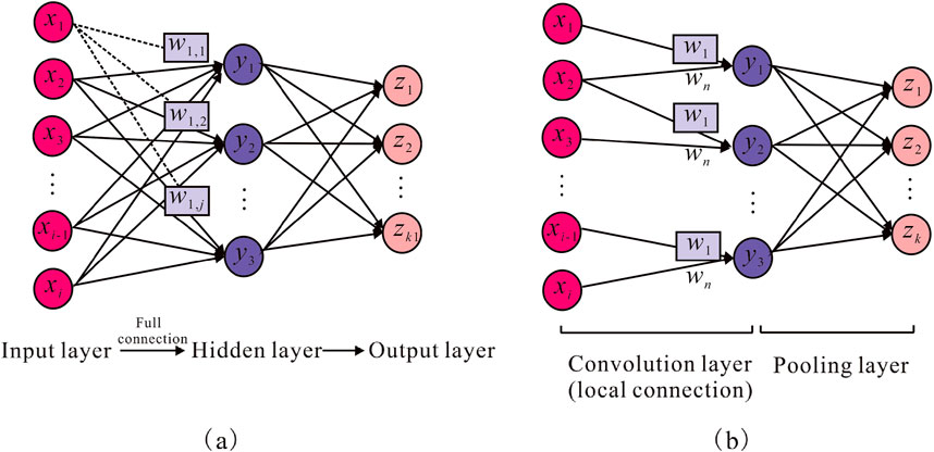
Figure 1. Network connection diagram of BP and 1D-CNN models. (a) Represents BP model; (b) represents 1D-CNN model.

The neurons of BP neural network are fully connected, and the corresponding weights and biases are varied. Hence, the output of the jth neuron in the hidden layer is represented as (Li et al., 2020):

$y_j=f\left({\displaystyle \sum _{i=1}^n}{w}_{i,j}{x}_i+b_j\right)(1)$

where x_i (i = 1, 2, .) is the input vector; f is the activation function; w_{i, j} is the weight from the ith neuron to the jth neuron; b_j is the bias of each neuron in the hidden layer.

Due to the introduction of convolution kernel in 1D-CNN model, the connection mode between neurons becomes local connection. So 1D-CNN model provides the feature of sharing weight. Then, the weight part of Equation 1 is improved to obtain the output of the jth neuron of the convolutional layer in 1D-CNN model:

$y_j=f\left({\displaystyle \sum _{i=1}^k}{w}_i{x}_{j-i+k}+b_k\right)(2)$

In Equation 2, w_i is the shared weight of convolutional kernel between neurons; k is the number of convolutional kernel; b_k is the offset corresponding to the kth convolutional kernel in the hidden layer.

2.2 Redefined S-ReLU function

To increase the nonlinear ability of CNN model, a novel function S-ReLU is created based on ReLU function and SoftPlus function. The advantages of S-ReLU are illustrated by analyzing its properties and comparing it to ReLU and SoftPlus, and then how S-ReLU propagates forward in the model is exhibited.

Glorot et al. (2011) were inspired by the performance of human brain neuron after stimulation in neuroscience and applied ReLU to the neural network for the first time. Through allowing CNN to simulate the workflow of biological neural networks, the expression ability was enhanced. The form of ReLU function is:

$f\left(x\right)=\left\{\begin{array}{l}x,x>0\\ 0,x\le 0\end{array}\right.(3)$

SoftPlus is considered to be a smooth approximation of ReLU, and they share many similarities (Hahnloser et al., 2003). The expression for SoftPlus is:

$f\left(x\right)=\text{In}\left(1+{\mathrm{e}}^{\mathrm{x}}\right)(4)$

The S-ReLU activation function is built using two types of activation functions stated in Equations 3, 4:

$f\left(x\right)=\left\{\begin{array}{l}x,x>0\\ x\left[e^x+x\text{In}\left(1+e^x\right)\right],x\le 0\end{array}\right.(5)$

As can be seen from Equation 5, the output is an identity function when x > 0, that is, the input is equal to the output. When x ≤ 0, the output is a combination of ReLU and SoftPlus functions. The derivative of S-ReLU activation function is:

$f\left(x\right)=\left\{\begin{array}{l}1,x>0\\ e^x+x\left(e^x+2\alpha +\frac{x{e}^x}{1+e^x}\right),x\le 0\end{array}\right.(6)$

Noted that α = ln (1+e^x) in Equation 6. Figure 2 presents S-ReLU function and derivative diagram. From f’+(0) = f’ (0) = 1, it can be inferred that f(x) is differentiable and its derivative is not a constant. Thus, f(x) is nonlinear, which will considerably improve the model’s ability to deal with complex problems.

Figure 2

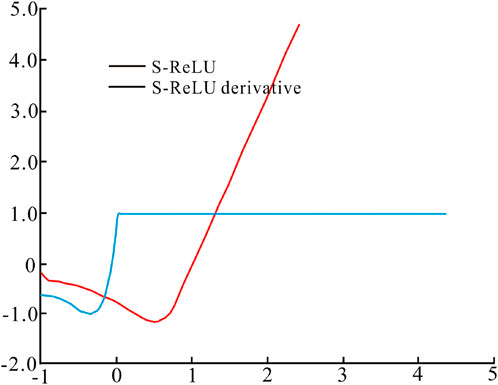
Figure 2. S-ReLU function and derivative diagram.

First of all, S-ReLU adds negative sample information. Specifically, S-ReLU contains positive and negative values, unlike SoftPlus, which always exists a value larger than 0 in the negative area. This significantly solves the “mean deviation” issue. S-ReLU is more in line with the characteristics of biological neuron response, which increases the anti-interference ability of the model. Secondly, when x approaches +$\infty$, f(x) approaches $\infty$. It is proved the function has no upper bound, which can accelerate the convergence speed of CNN model and avoid a sharp decrease in training speed after function saturation. When x approaches -$\infty$, f(x) approaches 0. It suggests that the function has a lower bound, making CNN model highly regularized and improving its robustness.

Additionally, S-ReLU function is composed of exponential function and logarithmic function, which is more complex than the function composed of only identity function (Equation 3). The operation makes S-ReLU function need more time in practical application. But the S-ReLU function can return a valid negative value during forward propagation, preventing the gradient from disappearing. The structure of S-ReLU function is extremely similar to that of ReLU function, which enables the S-ReLU function to possess several advantages of ReLU function, such as sparsity. This not only reduces the computational complexity of CNN model, but also enhances its expressive power, making the network more focused on the task itself.

2.3 Transformer encoder structure

Transformer structure is made up of multi-head self-attention mechanism and feedforward neural network (Figure 3). The Q (query matrix), K (key matrix) and V (value matrix) are the inputs of self-attention mechanism which is a special case of attention mechanism (Kumar et al., 2022). The sequence matches itself to extract the dependency between its parts. Equation 7 presents how each self-attention mechanism is calculated:

$\text{Attention}\left(Q,K,V\right)=\text{softmax}\left(\frac{Q{K}^{\mathrm{T}}}{\sqrt{d_k}}\right)V(7)$

where d_k is the dimension of channel. The Q and K use the inner product to match, and the result is an attention matrix whose value characterizes the correlation between Q and K. Multi-head self-attention mechanism employs multiple self-attention in parallel to learn the interdependence between different types of data, as shown in Equation 8 and Equation 9:

$\text{MultiHead}\left(Q,K,V\right)=\text{Concat}\left({\text{head}}_1,....{\text{head}}_h\right)W_o(8)$

$\begin{array}{l}{\text{head}}_i=\text{Attention}\left(Q{W}_i^Q,K{W}_i^K,V{W}_i^V\right)\\ W_i^Q\in R^{d_{\text{model}}\times d_k},W_i^K\in R^{d_{\text{model}}\times dk},W_i^V\in R^{d_{\text{model}}\times dv}\end{array}(9)$

Figure 3

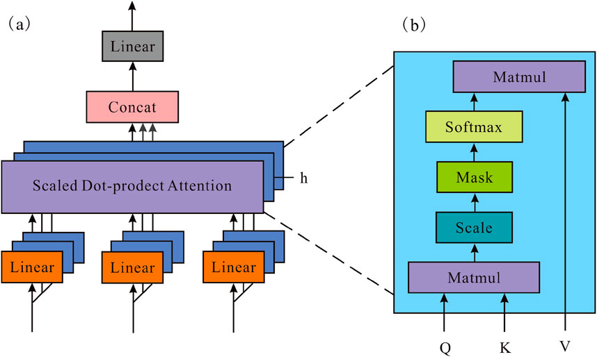
Figure 3. The construction of multi-head self-attention mechanism. (a) Multi-head self-attention mechanism, (b) Self-attention mechanism.

In this paper, h = 6 is selected, which is composed of six self-attention mechanisms.

Each layer in the Transformer encoder has a feedforward neural network, and the network is applied equally to each location. The structure includes the following linear transformations:

$FFN\left(x\right)=\max \left(0,x{W}_1+b_1\right)W_2+b_2(10)$

To avoid the problem of neuron “necrosis”, the S-ReLU function is in the middle of the structure of Equation 10. While linear transformations employ different parameters between layers, they are the same in all positions (Nawaz et al., 2020). Although linear transformations are the same in different positions, they adopt various parameters between layers (Liu et al., 2022). In Equation 7, due to the lack of position information, the position of self-attention layer is unknown. Consider adopting position self-attention mechanism, learnable relative position code is embedded. Each attention head can be expressed as Equation 11 through a trainable relative position code:

$\text{Attention}\left(Q,K,V\right)=\text{softmax}\left(\frac{Q{K}^{\mathrm{T}}}{\sqrt{d_k}}+\mathrm{B}\right)V(11)$

where B is the relative position code, which is a learnable parameter during network training.

2.4 Workflow of CNN-transformer model

The MBConv structure serves as the primary foundation for the convolution operation in the newly built model (Sivaanpu et al., 2024). Furthermore, the weighted values of the preset receptive field can be summarised to represent both the convolution operation and the self-attention process (Stojsic et al., 2024). The “inverted residual” design is used by both the Transformer encoder and the MBConv structure in the convolution layer. The design first employs 1 × 1 convolution to accomplish dimension augmentation, then 3 × 3 DW convolution is used to extract features, and finally 1 × 1 convolution is applied to achieve dimension reduction. This allows it to realize the mutual fusion of various feature data. The MBConv structure incorporates the S-ReLU activation function to expedite the network’s convergence.

Convolution specifically relies on the fixed convolution kernel to extract the feature data from the nearby receptive field. It not only assures that the learned convolution kernel responds most strongly to the local peculiarities of the input cased-hole information, but it also minimizes the model’s complexity. Local characteristics, on the other hand, tend to neglect the context correlation between distinct regions predicted by cased-hole parameters. By calculating the normalized weight based on pair similarity, the self-attention mechanism can immediately obtain global information. The global receptive field causes the model’s computation volume to grow quickly. In order to determine the feature information we wish to retain, CNN should extract the feature areas we are interested in prior to entering the Transformer encoder structure.

Combining the advantages of CNN and Transformer should be possible with the perfect model. Anti-interference performance enhancement of CNN-Transformer model is achieved through the use of S-ReLU activation function. The total structure is depicted in Figure 4. This model not only thoroughly extracts the feature regions of relevance for the prediction of cased-hole parameter, but it also gives more weight to significant feature information.

Figure 4

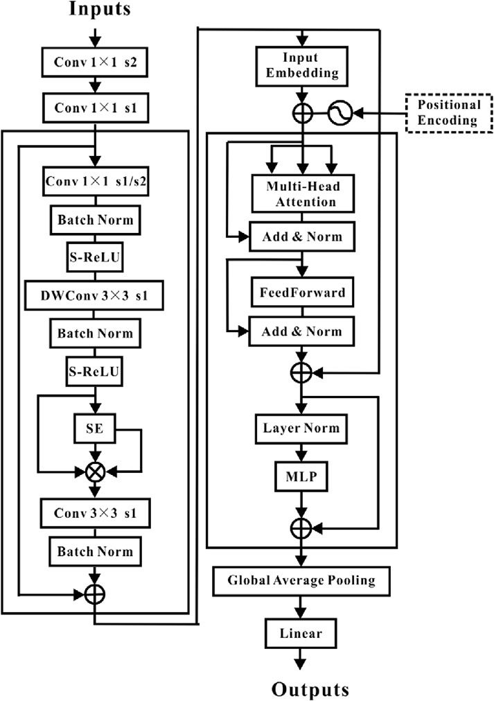
Figure 4. CNN-transformer structure schematic diagram.

2.5 Performance metrics evaluation

Pearson Correlation Coefficient (R) and Root-Mean-Square-Error (RMSE) are utilized to analyze the model’s predictive ability (Chen et al., 2020). R is the method to measure the correlation between two variables, and its value range is [-1, 1]. RMSE reflects the maximum error between target parameters and prediction parameters. Additionally, we conducted t-tests (Kim, 2015) on the prediction results of different models to statistically evaluate the differences between the models. Their calculation equations are as follows:

$R=\frac{C\text{ov}\left(Y,P\right)}{\sqrt{D\left(Y\right)}\sqrt{D\left(P\right)}}(12)$

$RMSE=\sqrt{{\sum }_{n=1}^N{\left(y_i-p_i\right)}^2\times \frac{1}{N}}(13)$

$t=\frac{\overline{p}\sqrt{k}}{\sqrt{\frac{{\sum }_{i=1}^k{\left(p^i-\overline{p}\right)}^2}{k-1}}}(14)$

In Equations 12, 13, Y and P denote the real and predicted parameter values; Cov (Y, P) and D denote the covariance and variance functions, respectively; y_i and p_i denote the true formation density and the predicted formation density; N denotes the samples’ number. In Equation 14, k is the iteration number. Pⁱ is the performance difference between different models in the ith iteration. $\overline{p}$ represents the average performance difference between different models.

3 Experiments

3.1 Data sample selection

A certain work area is located in the central western part of Ordos Basin, which is between two primary structural units: Tianhuan Depression and Shanbei Slope. Four detector density logging project was carried out in August 2019. This work area is mainly composed of dense sandstone, rich in pyrite, and has a geological thickness of 624–2014 m. The entire reservoir porosity ranges from 1.8% to 8.7%, with an average of 4.8%. The permeability ranges from 0.01 to 4.81 mD, with an average of 2.15 mD. The work area exhibits overall low porosity and low permeability characteristics. During the process of measuring formation density by the four-detector density logging instrument in this work area, the actual counting rates of different detectors with different energy windows were obtained at different depths by the gamma counters. For every detector counting rate of each energy window, ρ_b shows different features.

To establish the prediction model of formation density, the dataset samples mainly include six counting rates of energy window: 0–45 keV counting rate, 45–85 counting rate, 85–135 keV counting rate, 135–235 keV counting rate, 235–345 keV counting rate and 345–585 keV counting rate. The experimental data ratio of the training set, validation set and test set is set as 8:1:1. The training set data and validation set data used for the experiment were acquired from nine wells in the western part of work area, with a total of 1,680 samples and 210 samples, respectively. The purpose of the validation set is to prevent overfitting of the model. To ensure the generalization ability of the model, the test set selects regions that are different from the training set. The predicted sample data comes from three wells in the south, with a total of 210 samples.

3.2 Data preprocessing

Before data preprocessing, the quality control of logging data was strictly implemented by adopting standardized acquisition process, high-precision instrument calibration and double review to ensure accurate data entry. Due to environmental interference or errors in the acquisition process, the obtained detector counting rate may be affected by noise interference, which results in the occurrence of outliers. The box plot method is used for outlier detection (He et al., 2023). Data with less than Q1-1.5*IQR or greater than Q3 + 1.5*IQR are defined as potential outliers, as shown in Figure 5. Among them, Q1 and Q3 are the 25th and 75th percentile values of the data, respectively, and IQR is the interquartile range (Q3-Q1). For detected potential outliers, further verification should be applied based on professional knowledge. Considering the limited amount of experimental data, the confirmed outliers will be treated as missing values to avoid potential information loss. K-Nearest Neighbor (KNN) interpolation method is adopted to fill missing values and preserve data information to the maximum extent. The KNN method estimates and fills missing values by searching for several most similar historical data near the missing values, which can effectively handle missing value problems in multivariate datasets while maintaining data distribution characteristics. The specific KNN interpolation steps are as follows. Firstly, for each sample containing missing values, select the K samples closest to the missing sample based on metrics such as Euclidean distance (K = 4 in this study). Secondly, use the weighted average of these K sample data to fill in missing values, with weights inversely proportional to the samples. Finally, replace data points that do not meet the requirements or outliers that deviate from normal data can reduce the interference of logging noise.

Figure 5

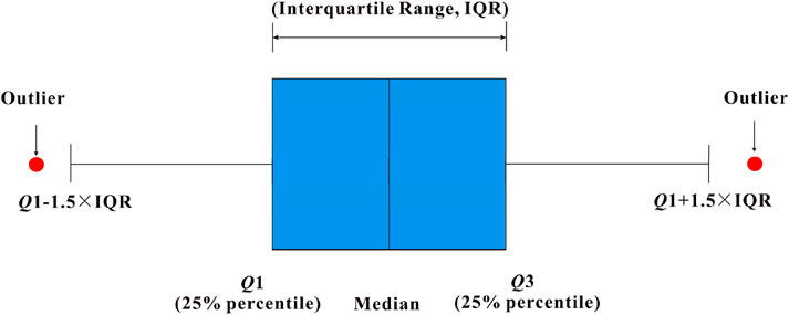
Figure 5. Schematic diagram of box plot method.

3.3 Feature selection and data standardization

Based on the fundamental theory of density logging, there is a relationship between the cased-hole parameters and the counting rate of every energy window. Six energy windows of the detectors with a source distance of 16.84 cm were chosen for feature selection. The purpose is to reduce the redundant feature information and lower the model complexity. Figure 6 examines the relationship between ρ_b and the energy window counting rate.

Figure 6

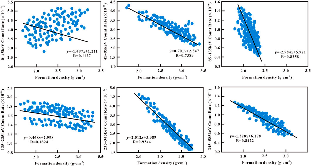
Figure 6. Correlation analysis of formation density and the counting rate of six energy windows.

It is observed that there is a high correlation between ρ_b and the counting rates in the energy windows of 45–85 keV, 85–135 keV, 235–345 keV and 345–585 keV. They have the correlation coefficients (R) above 0.5. Furthermore, the correlation coefficients (R) of ρ_b with the counting rates of 0–45 keV and 135–235 keV energy windows are less than 0.3 and do not exhibit any significant correlation. Thus, we consider the four counting rates (45–85 keV, 85–135 keV, 235–345 keV and 345–585 keV) for various detector energy windows to be the input values. The goal is to simply develop the nonlinear mapping between energy window counting rate and formation density.

Before inputting the counting rate of detector into CNN-Transformer model, the data must be standardized first. To eliminate the magnitude difference between counting rate data and ensure that the data with small magnitude will not be submerged during the modeling process, we standardize all the data with z-score method. The specific calculation process is shown in Equation 15.

$x_i=\frac{x-x_{\min }}{x_{\max }-x_{\min }}(15)$

where x_i is the standardized counting rate; x is the real counting rate; x_min and x_max are the minimum and maximum values of counting rate.

3.4 Experimental setup

In the experiment, the processor is Intel (R) Xeon (R) CPU E5-2687 W v4 at 3.00GHz, the graphics card is NVIDIA Ge Force RTX 3090, the running memory is 24 GB, the GPU acceleration library is CUDA11.1, and the deep learning framework is PyTorch. The model training adopts cross entropy loss as the loss function and updates the learnable model parameters by the AdamW optimizer. AdamW optimizer combines Adam optimizer and weight decay, which not only has the advantage of adaptive learning rate, but also effectively prevents overfitting through weight decay. In addition, an early stopping strategy was introduced during the training process. L2 regularization and Dropout technique were also used to control model complexity and enhance the model’s generalization ability.

During the construction process of CNN-Transformer model, optimizing algorithm hyperparameters is a key step to ensure superior model performance. This study adopted Bayesian optimization algorithm combined with K-fold cross validation to adjust the model hyperparameters for optimal predictive performance. Figure 7 displays the changes in the loss function value and accuracy value (Sang et al., 2021) as iteration number increases during the training process. At the beginning of training, the loss function value experienced a rapid decline. When the iteration number reached around 150, the model gradually converged. The loss function value tended to stabilize, and the accuracy value reached its highest level. Table 1 provides a detailed list of the optimization results for the key hyperparameters in the CNN-Transformer model. Besides, the traditional inversion model of Wu et al. (2017) in the Introduction section, CNN model of Cai (2022) and Transformer model are used as a comparison. The experimental environment of the comparative models is identical, the same method is used to ensure optimal hyperparameters, and training is also conducted on the same dataset.

Figure 7

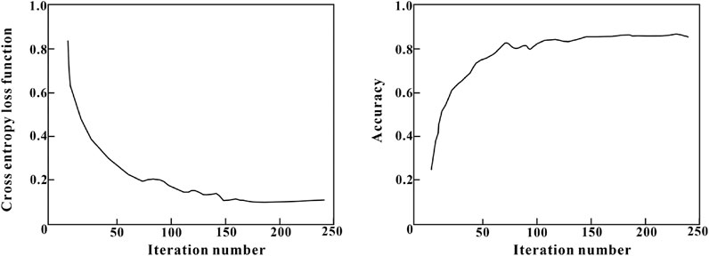
Figure 7. The variation of loss function value and accuracy vale with the number of iterations.

Table 1

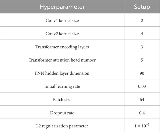
Table 1. Optimization results of key hyperparameters in the CNN-transformer model.

4 Example and results

4.1 Cased-hole formation density prediction performance

The prediction results of formation density by CNN-Transformer model, Transformer model, CNN model and traditional inversion model (Wu et al., 2017) are illustrated in Figure 8. The true density value was measured through geochemical methods from real rock samples of the test wells, with a sampling interval of 0.5 m.

Figure 8

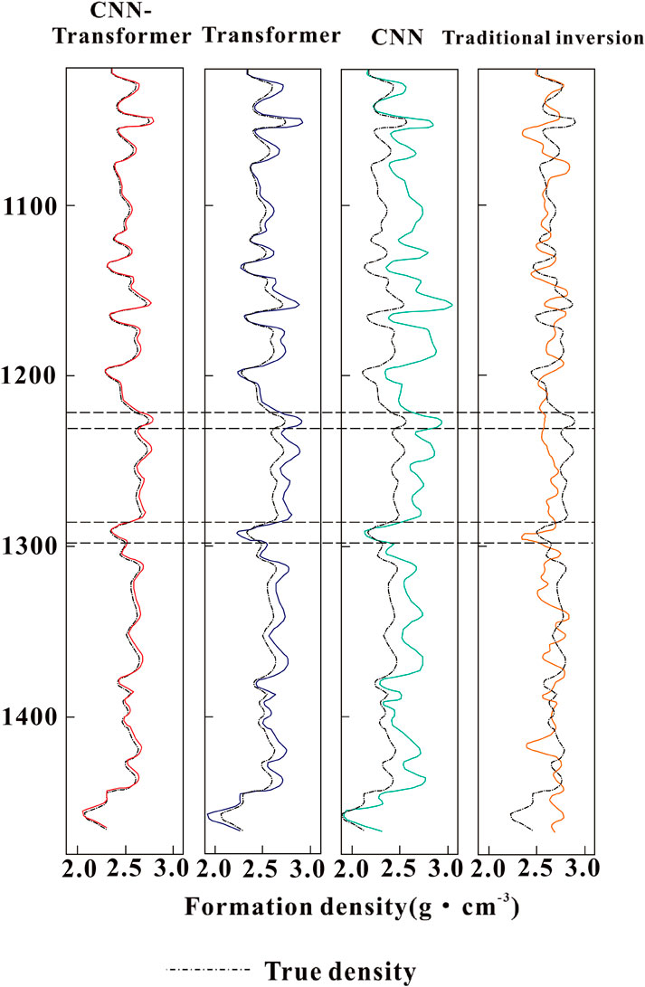
Figure 8. The predicted curves of formation density based on different models in the test set. The black dotted curve represents the true density value. The red curve represents the prediction result of CNN-Transformer model, the blue curve represents the prediction result of Transformer model, the green curve represents the prediction result of CNN model, and the orange curve represents the prediction result of traditional inversion model.

From Figure 8, it is clear that the four models all offer satisfactory prediction performance on formation density curves with depth, indicating that artificial intelligence models can effectively extract the temporal and nonlinear features of counting rate data. On the one hand, it appears that the prediction results of CNN model are relatively smooth and do not accurately depict the local mutation of true density curves. Then comparing traditional inversion model to CNN model, its prediction performance is noticeably inferior. Conversely, the values predicted by Transformer and CNN-Transformer models are more in line with true values. The intersection findings between the true density values in the test set and the predicted density values are displayed in Figure 9 to perform comparison analysis. It can be determined that there is a strong correlation between the true formation density and the predicted formation density derived from CNN-Transformer and Transformer models. The aforementioned investigation demonstrates that CNN-Transformer and Transformer models featuring long-term memory function are superior to traditional machine learning models in their ability to forecast the formation density.

Figure 9

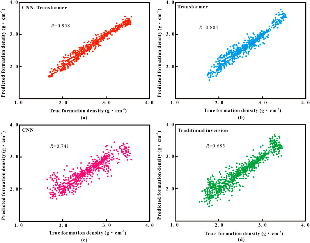
Figure 9. The intersection results between the predicted density values and true density values in the test set. (a) CNN-Transformer model, (b) Transformer model, (c) CNN model, (d) Traditional inversion model.

Besides, CNN-Transformer and Transformer models’ output results do not differ much when the formation density curve changes smoothly. The reason for this is that when the change is stable, the formation density curve lacks a clear local shape. CNN-Transformer model predicts density values that are closer to reality than Transformer model when there is a local mutation in the formation density curve. For instance, it is obvious that CNN-Transformer model accurately predicts this mutation while traditional inversion model, CNN model and Transformer model typically fail to forecast at the depth of 1,230–1,240 m and 1,288–1,298 m. As for the prediction results of local features, CNN-Transformer model also outperforms ordinary Transformer model. Because CNN-Transformer has the advantages of both CNN and Transformer models, which plays a role in accurately extracting local data features.

Additionally, Table 2 shows the accuracy indicators of several models’ predictions for formation density. From the table, CNN-Transformer model can achieve R and RMSE of 0.908 and 0.079 for 1,680 training sample sets. 210 test samples have R and RMSE values up to 0.958 and 0.049, respectively. According to statistics, the R value of CNN-Transformer model rises throughout the entire training set than traditional inversion model, CNN model and Transformer model by 46.22%, 25.76% and 9.53%. Compared to traditional inversion model, CNN model and Transformer model, CNN-Transformer model’s RMSE value is reduced by 81.54%, 66.38% and 52.98%, respectively. In the test set, the R-value of CNN-Transformer model is higher than traditional inversion model, CNN model and Transformer model for the entire test set by 40.29%, 29.28% and 19.15%, respectively. Compared with the traditional inversion model, CNN model and Transformer model, CNN-Transformer model’s RMSE value drops by 86.27%, 77.52% and 71.84%. High R value and low RMSE value are the two primary markers of small variation for formation density prediction. It demonstrates that CNN-Transformer model’s fitting curve more closely matches the real circumstances.

Table 2

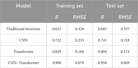
Table 2. Performance metrics of the prediction models.

To verify whether the prediction performance of CNN-Transformer model is greatly better than other comparison models in a statistical sense, we conducted paired t-test. Assuming zero hypothesis H₀ is that the prediction performance of CNN-Transformer model is superior to the corresponding comparison model, and the threshold is set to 0.05. A larger p-value confirms H₀, while a smaller p-value negates H₀. The t-test results regarding the model performance comparison are shown in Table 3. It reports the significance of all methods at the sampling ratios of 1:10, 1:50, 1:100 and 1:200. From the t-test results, it is obvious that H = 0 was all obtained at different sampling ratios. Statistically, this fact proves that CNN-Transformer offers significantly improved predictive performance compared with other comparison models.

Table 3

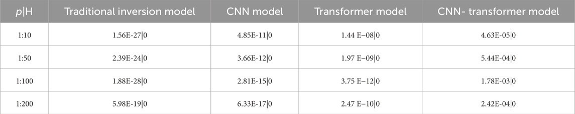
Table 3. The t-test results of CNN-transformer and other comparison models on the test data.

4.2 Model practicality

In terms of operational efficiency, deep learning methods for predicting formation density provide unique advantages over conventional methods. In contrast, deep learning methods only require sending data into the network for computation, and can be completed in a very short time with the support of GPU parallelism. According to the experimental results, we measured the computation time of the corresponding model under the optimal hyperparameter setting, and the comparison results are presented in Figure 10. Table 4 lists the size and computational complexity of different models.

Figure 10

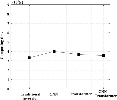
Figure 10. The calculation time comparison.

Table 4

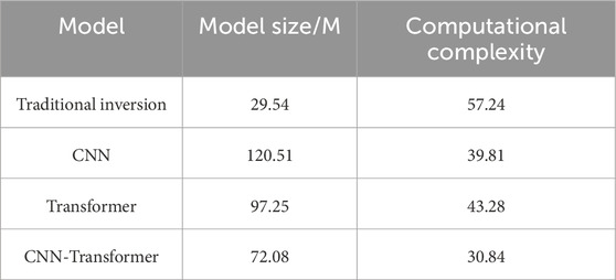
Table 4. The size and computational complexity of four models on the dataset.

It is worth noting that due to the use of more network structures in the CNN- Transformer model, there may be an increase in computation time. But from Figure 10, it can be seen that the computational time difference between four methods is not big. Then combining Figure 10 and Table 4, the inference time is faster, the computational complexity (GFLOPs) is lower, and it is lighter compared with several mainstream networks. Overall, CNN-Transformer model not only ensures the model accuracy in predicting formation density, but also reduce the amount of calculation.

4.3 Sensitivity analysis

During the data set regression, the feature importance scores of each model are calculated using the Shapley Additive exPlanations (SHAP) approach (Lundberg and Lee, 2017). This approach mainly highlights the average impact of each feature on the model output. The average values of these importance scores are shown in Table 5. Most models have similar feature rankings: 45–85 keV counting rate, 235–345 keV counting rate, 345–585 keV counting rate, 85–135 keV counting rate. The importance difference between the first feature (45–85 keV counting rate) and the second feature (235–345 keV counting rate) is much smaller than the difference between the third feature (345–585 keV counting rate) and the fourth feature (85–135 keV counting rate). It indicates that the 45–85 keV counting rate and 345–585 keV counting rate offer a more significant impact on the prediction process of CNN-Transformer model.

Table 5

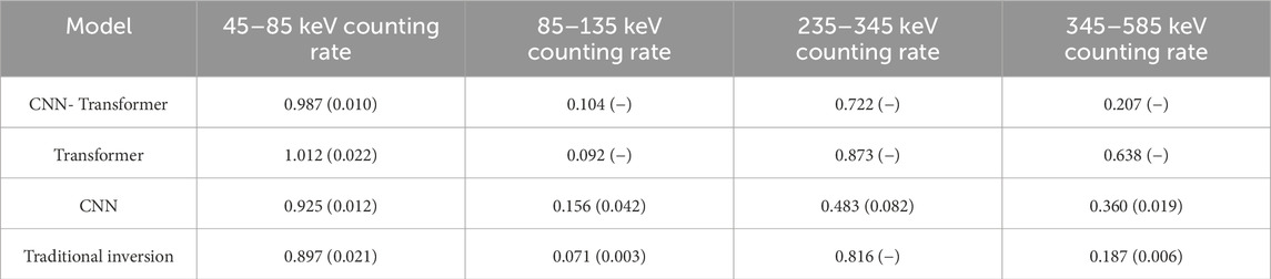
Table 5. The feature importance (SHAP) score for the regression test dataset of each model.

Figure 11 plots the score values, which can be better visualized by feature importance and differences. According to Figure 11 W1 has the highest score. That can be inferred that the 45–85 keV energy window counting rate gets the greatest influence on formation density prediction. Additionally, its value is positive, which means that increasing this parameter will greatly enhance the prediction ability of formation density.

Figure 11

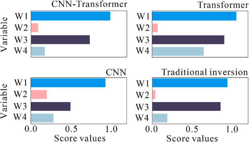
Figure 11. Feature importance based on SHAP score.

5 Discussion

The contribution of this study is to explore the feasibility of using the detector counting rate during the well logging process to predict formation density by CNN-Transformer model. It also demonstrates the superiority of CNN-Transformer model in this situation. Compared with previous literature on predicting formation density, the accuracy has been greatly enhanced.

When using the traditional density inversion method (Li et al., 2017; Wu et al., 2017) to obtain formation density, it was found that although direct inversion of formation density can be achieved through the difference in counting rates of multiple detectors and the theoretical model is clear, it requires complex wellbore compensation correction process, and the inversion error increases with the complexity of the environment. The Terzaghi calibration model (Cao et al., 2024) does not require GPU training or large-scale data storage, but the selection of scanning line direction depends on experience or prior knowledge (such as the direction of geostress), and subjective errors may affect the inversion accuracy. This is also the reason why we did not adopt this method in the model comparison stage. When using CNN model (Cai, 2022) to predict formation density, although the computational efficiency is high and the structure is easy to tune, it is difficult to achieve the optimal balance between efficiency and accuracy. When using the proposed CNN-Transformer model to predict formation density, although the computational complexity of the model is high, extracting local features of well logging data through convolutional layers (such as formation abrupt intervals) and capturing long sequence dependencies using the Transformer’s self-attention mechanism make up for the shortcomings of CNN in modeling global information. The error value does not change with the complexity of the environment.

Compared to the other methods, the advantages of using CNN-Transformer model for predicting formation density mainly lie in the ability to extract richer feature information, achieve long-term high-precision prediction, and improve prediction efficiency and accuracy. Besides, this study provides an accurate solution for reservoir parameter prediction, which greatly improves its practical application in oil and gas exploration. Our model can quickly determine the formation density, which helps to significantly reduce exploration cost. This practical innovation enables industry professionals to make smarter, more sustainable decisions that optimize resource utilization during exploration and development. However, there are still many disadvantages and areas for improvement. Firstly, the density distribution of some formation may be sparse, which makes it difficult for models to accurately learn the characteristics of these regions. Secondly, CNN-Transformer model is primarily data-driven, and the formation physics model (such as gamma absorption formula or formation density change rule) is not introduced, which may lead to physical inconsistency of prediction results. Finally, real formations are diverse and heterogeneous, and models may be difficult to generalize to complex geological conditions. Thus, balancing the sample distribution, embedding the gamma absorption physics model in the model design, and input the geological background into the network model are a field worthy of further study.

6 Conclusion

To accomplish the goal of automatic formation density prediction and solve the insufficient feature extraction ability problem of CNN model under multiple logging data conditions, this paper offers a network model for cased-hole formation density prediction by combining the benefits of CNN and Transformer. After extracting our desired feature areas from CNN, we utilize the Transformer encoder to provide regions of interest high weights, allowing us to concentrate on important areas and features. Thus, CNN model’s accuracy in classification is improved. The CNN-Transformer model also incorporates the new S-ReLU function to avoid the problem of neuron “necrosis”. Following data parameter optimization, the CNN-Transformer model’s inputs are chosen from the counting rates of four energy windows (45–85 keV, 85–135 keV, 235–345 keV and 345–585 keV) for each detector during the well logging process. The proposed CNN-Transformer model is compared with traditional inversion model, CNN model and Transformer model in terms of prediction accuracy. On the test set, the predicted formation density of CNN-Transformer model showed excellent consistency with the actual measured values, with an R of 0.958 and an RMSE of 0.049. The paired t-test also strengthens the argument for the superiority of CNN-Transformer model statistically. Meantime, it reveals that the 45–85 keV counting rate contributes the most to the formation density prediction through the interpretability analysis of SHAP method. This study provides a reliable and fast approach for predicting formation density. ‌The next step of research will embed a gamma absorption physics model in the model design, input geological background into the network model, and further enhance prediction accuracy.

Data availability statement

The raw data supporting the conclusions of this article will be made available by the authors, without undue reservation.

Author contributions

XC: Writing – review and editing, Writing – original draft. HZ: Writing – review and editing, Methodology.

Funding

The author(s) declare that no financial support was received for the research and/or publication of this article.

Conflict of interest

The authors declare that the research was conducted in the absence of any commercial or financial relationships that could be construed as a potential conflict of interest.

Generative AI statement

The author(s) declare that no Generative AI was used in the creation of this manuscript.

Publisher’s note

All claims expressed in this article are solely those of the authors and do not necessarily represent those of their affiliated organizations, or those of the publisher, the editors and the reviewers. Any product that may be evaluated in this article, or claim that may be made by its manufacturer, is not guaranteed or endorsed by the publisher.

References

Abo-Tabik, M., Costen, N., Darby, J., and Benn, Y. (2020). Towards a smart smoking cessation app: a 1D-CNN model predicting smoking events. Sensors 20 (4), 1099. doi:10.3390/s20041099

PubMed Abstract | CrossRef Full Text | Google Scholar

Al-Mudhafar, W. J., Abbas, M. A., and Wood, D. A. (2023). Integration of electromagnetic, resistivity-based and production logging data for validating lithofacies and permeability predictive models with tree ensemble algorithms in heterogeneous carbonate reservoirs. Petrol. Geosci. 30 (1), 114–120. doi:10.1144/petgeo2023-067

CrossRef Full Text | Google Scholar

Barkataki, N., Tiru, B., and Sarma, U. (2022). A CNN model for predicting size of buried objects from GPR B-Scans. J. Appl. Geophys. 200, 104620–265. doi:10.1016/J.JAPPGEO.2022.104620

CrossRef Full Text | Google Scholar

Cai, S. (2022). Study on response characteristics of high-resolution density logging and multi-parameter evaluation method of cased holes. Lanzhou Univ., 87–98.

Google Scholar

Cao, D. S., Zeng, L. B., Gomez-Rivas, E., Gong, L., Liu, G., Lu, G., et al. (2024). Correction of linear fracture density and error analysis using underground borehole data. J. Struct. Geol. 184, 105152. doi:10.1016/j.jsg.2024.105152

CrossRef Full Text | Google Scholar

Cresson, R. (2019). A framework for remote sensing images processing using deep learning techniques. IEEE Geosci. Remote Sens. Lett. 16 (01), 25–29. doi:10.1109/LGRS.2018.2867949

CrossRef Full Text | Google Scholar

Dawoon, L., Sungryul, S., Woohyun, S., and Wookeen, C. (2022). Zero-offset data estimation using CNN for applying 1D full waveform inversion. J. Geophys. Eng. 19 (01), 39–50. doi:10.1093/JGE/GXAB072

CrossRef Full Text | Google Scholar

Ekechukwu, G., and Adejumo, A. (2024). Explainable machine-learning-based prediction of equivalent circulating density using surface-based drilling data. Sci. Rep. 14 (1), 17780–17789. doi:10.1038/s41598-024-66702-w

PubMed Abstract | CrossRef Full Text | Google Scholar

Feng, G., Liu, W. Q., and Yang, Z. (2024). Shear wave velocity prediction based on 1DCNN-BiLSTM network with attention mechanism. Front. Earth Sci. 12, 1376344. doi:10.3389/feart.2024.1376344

CrossRef Full Text | Google Scholar

Glorot, X., Bordes, A., and Bengio, Y. (2011). Deep sparse rectifier neural networks. J. Mach. Learn. Res. 15, 315–323.

Google Scholar

Hahnloser, R. R., Seung, H. S., and Slotine, J. J. (2003). Permitted and forbidden sets in symmetric threshold-linear networks. Neural. Comput. 15 (3), 621–638. doi:10.1162/089976603321192103

PubMed Abstract | CrossRef Full Text | Google Scholar

Hassaan, S., Ibrahim, F. A., Mohamed, A., and Elkatatny, S. (2024). Prediction of formation permeability while drilling: machine learning applications. Arab. J. Sci. Eng., 1–14. doi:10.1007/s13369-024-09864-z

CrossRef Full Text | Google Scholar

He, L., Li, G., Wu, X., Zhang, S., Tian, M., Li, Z., et al. (2023). Characteristics of NO_x and NH₃ emissions from in-use heavy-duty diesel vehicles with various aftertreatment technologies in China. J. Hazard Mater 465, 133073. doi:10.1016/j.jhazmat.2023.133073

PubMed Abstract | CrossRef Full Text | Google Scholar

Huang, L., and Xia, Y. (2019). Joint blur kernel estimation and CNN for blind image restoration. Neurocomputing 396 (3), 324–345. doi:10.1016/j.neucom.2018.12.083

CrossRef Full Text | Google Scholar

Jin, C., and Tong, C. (2023). Remote sensing image classification method based on CNN and Transformer structure. Lasters Optoelectron. Prog. 31, 1–16.

Google Scholar

Johnson, E., Obot, O., Attai, K., Akpabio, J., and Inyang, U. G. (2023). The use of machine learning in oil well petrophysics and original oil in place estimation: a systematic literature review approach. J. Eng. Res. Rep., 157–167.

Google Scholar

Khisamutdinov, A. I., and Pakhotina, Y. A. (2015). Transport equation and evaluating formation parameters based on gamma-gamma log data. Russ. Geol. Geophys. 56 (09), 1357–1365. doi:10.1016/j.rgg.2015.08.011

CrossRef Full Text | Google Scholar

Kim, S., Lee, K., Lee, M., Lee, J., Ahn, T., and Lim, J. (2021). Evaluation of saturation changes during gas hydrate dissociation core experiment using deep learning with data augmentation. J. Pet. Sci. Eng. 209, 109820. doi:10.1016/J.PETROL.2021.109820

CrossRef Full Text | Google Scholar

Kim, T. K. (2015). T test as a parametric statistic. Korean J. Anesthesiol. 68 (6), 540. doi:10.4097/kjae.2015.68.6.540

PubMed Abstract | CrossRef Full Text | Google Scholar

Kumar, S., Kumar, A., and Lee, D. G. (2022). Semantic segmentation of UAV images based on Transformer framework with context information. Mathematics 24 (03), 4735–26. doi:10.3390/MATH10244735

CrossRef Full Text | Google Scholar

Lei, J. W., Fang, H. Y., Zhu, Y. N., Chen, Z. Q., Wang, X., Xue, B., et al. (2024). GPR detection localization of underground structures based on deep learning and reverse time migration. NDT&E Int. 143, 103043. doi:10.1016/j.ndteint.2024.103043

CrossRef Full Text | Google Scholar

Li, T., Zuo, R., Xiong, Y., and Peng, Y. (2020). Random-drop data augmentation of deep convolutional neural network for mineral prospectivity mapping. Nat. Resour. Res. 30 (1), 27–38. doi:10.1007/s11053-020-09742-z

CrossRef Full Text | Google Scholar

Li, X., Xiao, C., and Huang, R. (2017). Three-detector density logging tool for measuring casing thickness and cement sheath density. Well Logging Technol. 41 (03), 305–309.

Google Scholar

Liang, L., Lei, T., Donald, A., and Blyth, M. (2021). Physics-driven machine-learning-based borehole sonic interpretation in the presence of casing and drillpipe. SPE Reserv. Eval. Eng. 24 (2), 310–324. doi:10.2118/201542-PA

CrossRef Full Text | Google Scholar

Lim, B., Yu, H., Daeung, Y., and Nam, M. J. (2021). Machine learning derived AVO analysis on marine 3D seismic data over gas reservoirs near South Korea. J. Pet. Sci. Eng. 197, 108105. doi:10.1016/J.PETROL.2020.108105

CrossRef Full Text | Google Scholar

Liu, L., Kong, G., Duan, X., Long, H., and Wu, Y. (2022). Siamese network with transformer and saliency encoder for object tracking. Appl. Intell. 53 (02), 2265–2279. doi:10.1007/S10489-022-03352-3

CrossRef Full Text | Google Scholar

Lundberg, S., and Lee, S. (2017). A unified approach to interpreting model predictions. No. 31 Int. Conf. Neural Inf. Process. Syst., 4768–4777.

Google Scholar

Madan, P., Singh, V., Chaudhari, V., Albagory, Y., Dumka, A., Singh, R., et al. (2022). An optimization-based diabetes prediction model using CNN and Bi-directional LSTM in real-time environment. Appl. Sci. 12 (8), 3989–125. doi:10.3390/APP12083989

CrossRef Full Text | Google Scholar

Majid, B., and Hadi, R. (2019). Reservoir rock permeability prediction using SVR based on radial basis function kernel. Carbonate. Evaporite. 34 (3), 699–707. doi:10.1007/s13146-019-00493-4

CrossRef Full Text | Google Scholar

Nawaz, A., Huang, Z., Wang, S., Akbar, A., and Gumaei, A. (2020). Gps trajectory completion using end-to-end bidirectional convolutional recurrent encoder-decoder architecture with attention mechanism. Sensors 20 (18), 5143–5181. doi:10.3390/s20185143

PubMed Abstract | CrossRef Full Text | Google Scholar

Ozcanli, A. Z., and Baysal, M. (2022). Islanding detection in microgrid using deep learning based on 1D CNN and CNN-LSTM networks. Sustain. Energy Grids 32, 100839. doi:10.1016/J.SEGAN.2022.100839

CrossRef Full Text | Google Scholar

Pham, N., Wu, X. M., and Naeini, E. Z. (2020). Missing well log prediction using convolutional long short-term memory network. Geophysics 85 (4), WA159–WA171. doi:10.1190/geo2019-0282.1

CrossRef Full Text | Google Scholar

Rizvi, S. H. (2021). Time series deep learning for robust steady-state load parameter estimation using 1D-CNN. Arab. J. Sci. Eng. 47, 2731–2744. doi:10.1007/s13369-021-05782-6

CrossRef Full Text | Google Scholar

Ronald, P., Laurent, M., and James, H. (2011). Formation density measurements in cased wellbore. Petrophysics 52 (02), 96–107.

Google Scholar

Sang, K. H., Yin, X. Y., and Zhang, F. C. (2021). Machine learning seismic reservoir prediction method based on virtual sample generation. Petrol Sci. 18 (6), 1662–1674. doi:10.1016/j.petsci.2021.09.034

CrossRef Full Text | Google Scholar

Sivaanpu, A., Punithakumar, K., Zheng, R., Noga, M., Ta, D., Lou, E. H. M., et al. (2024). Speckle noise reduction for medical ultrasound images using hybrid CNN-Transformer network. IEEE Access 12, 168607–168625. doi:10.1109/ACCESS.2024.3496907

CrossRef Full Text | Google Scholar

Stojsic, K., Rigo, D. M., and Jurkovic, S. (2024). Automated vertebral bone quality determination from T1-weighted lumbar spine MRI data using a hybrid Convolutional Neural Network-Transformer neural network. Appl. Sci. 14 (22), 10343. doi:10.3390/app142210343

CrossRef Full Text | Google Scholar

Sun, Y., Zeng, Q., Geng, B., Lin, X., Sude, B., and Chen, L. (2019). Deep learning architecture for estimating hourly ground-level PM2.5 using satellite remote sensing. IEEE Geosci. Remote Sens. Lett. 16, 1343–1347. doi:10.1109/lgrs.2019.2900270

CrossRef Full Text | Google Scholar

Wang, J., Cao, J., Yuan, S., Xu, H., and Zhou, P. (2024). Porosity prediction using a deep learning method based on bidirectional spatio-temporal neural network. J. Appl. Geophys. 228, 105465. doi:10.1016/j.jappgeo.2024.105465

CrossRef Full Text | Google Scholar

Williams, J., Singh, J., Kumral, M., and Ramirez Ruiseco, J. (2021). Exploring deep learning for dig-limit optimization in open-pit mines. Nat. Resour. Res. 30 (1), 2085–2101. doi:10.1007/s11053-021-09864-y

CrossRef Full Text | Google Scholar

Wu, W., Chen, B., Yu, G., Li, M., and Li, X. (2017). Responses and data inversion of four-detector scattered-gamma-ray logging in cased holes. J. Pet. Sci. Eng. 159 (04), 691–701. doi:10.1016/j.petrol.2017.10.001

CrossRef Full Text | Google Scholar

Xiangyang, J. Q., Fan, J. L., and Zhang, Q. (2024). Research on optimization of X-ray density meter's ray exit angle. Well Logging Technol. 48 (06), 772–780+788. doi:10.16489/j.issn.1004-1338.2024.06.005

CrossRef Full Text | Google Scholar

Xiao, X., Yan, J., and Guo, W. (2023). Prediction method of sweet spot parameters in shale gas reservoirs based on LightGBM algorithm. Coal Geol. China 35 (10), 28–37.

Google Scholar

Zheng, H. (2008). A new model of cement density-casing wall thickness logging interpretation. Well Logging Technol. 30 (4), 243–252.

Google Scholar

Zhou, H., Zheng, L., and Fan, J. (2002). Application of generalized regression neural network in the prediction of ash melting point. J. Zhejiang Univ. Eng. Sci. 102 (11), 90–93.

Google Scholar

Zulfiqar, A. K., Tanveer, H., Amin, U., Seungmin, R., Lee, M., and Baik, S. W. (2020). Towards efficient electricity forecasting in residential and commercial buildings: a novel hybrid CNN with a LSTM-AE based framework. Sensors 20 (5), 102–111. doi:10.3390/s20051399

CrossRef Full Text | Google Scholar