Multi-source landslide inventories for susceptibility assessment: a case study in the Concepción Metropolitan Area, Chile

The Concepción Metropolitan Area (CMA) in South-Central Chile presents a complex interplay of climatic conditions, tectonic activity, and varied topography that heightens landslide susceptibility. The CMA is characterized by steep escarpments and sloping valleys atop tectonic blocks. This complex setting creates landslide-prone areas as urban development extends into unstable hillslopes. Unfortunately, current landslide inventories are limited and inconsistent, hindering effective susceptibility zoning and urban planning efforts. The objective of this study was to improve quantitative landslide susceptibility assessments in the CMA by developing a comprehensive landslide inventory spanning from 1990 to 2023. The methods we implemented included compiling a multitemporal and multi-source comprehensive landslide inventory for the CMA, integrating historical and recent data. The inventory consolidates detailed records from the Chilean Geological Survey (SERNAGEOMIN), encompassing materials, conditioning factors, anthropogenic influences, and other relevant variables. To test the potential of our inventory for landslide susceptibility, we compared its performance relative to existing compilations using the Frequency Ratio method. Three slide susceptibility models were compared, two using previous databases, and one using the inventory developed in this study. A comparative analysis highlighted differences in predictive accuracy due to inventory completeness. Our findings show that the model using our landslide inventory exhibited the highest predictive accuracy and spatial specificity, emphasizing the benefits of a detailed, curated landslide inventory for more reliable localized assessments. Additionally, this study is novel for the region and shows that detailed inventories significantly improve accuracy of landslide susceptibility models, providing a more reliable foundation for risk-informed urban planning and land-use management in vulnerable regions.

1 Introduction

Landslides are gravitational processes that displace volumes of rock, debris, or soil lower elevations at varying velocities (Cruden and Varnes, 1996), controlled by site-specific conditions and triggering factors. Site conditions include geological and geotechnical conditions, geomorphological characteristics, soil types, land use (e.g., vegetation, urban development), hydrogeology, and anthropogenic activity (Highland and Bobrowsky, 2008). Triggering factors alter the stability of the terrain (McColl, 2022), typically corresponding to precipitation (Polemio and Petrucci, 2000; Froude and Petley, 2018) and seismicity (Keefer, 2002; Tatard et al., 2010).

With more than 4,800 events causing several thousand fatalities, from 2004 to 2016, landslides are one of the most life-threatening hazards globally (Froude and Petley, 2018). To mitigate and reduce the impact of these phenomena, inventories that capture key aspects of landslide occurrence, characteristics, and spatial distribution are essential for quantitative assessments of susceptibility and zoning (van Westen et al., 2008). Inventories are necessary to determine regional distribution, movement’s types affecting specific areas, identify patterns of triggering factors, allowing estimations of landslide recurrence and damaging potential (van Westen et al., 2008; Fell et al., 2008; Guzzetti et al., 2012; Tyagi et al., 2022). However, in order to be effective, inventories should provide a wide range of information, including location of landslide events, occurrence dates and frequency, movement type, failure mechanisms, causal factors, displaced volumes, damage caused or magnitude, validation metrics, data uncertainties and their potential sources (van Westen et al., 2008; Fell et al., 2008; Guzzetti et al., 2012). Inventories are typically maps or geodatabases that display these landslide attributes in a spatially distributed fashion, making them useful for planning studies.

Inventory maps are classified as archive or geomorphological (Guzzetti et al., 2012). An archive inventory contains information collected from bibliographic sources or technical reports, while geomorphological inventories can be further classified into (i) historical, containing cumulative effects of many landslide events over a period of tens, hundreds or thousands of years; (ii) event-based, showing landslides caused by a single trigger, such as an earthquake or a rainfall event; (iii) seasonal, characterizing landslides caused by one or several events during one or several seasons; and (iv) multi-temporal, depicting landslides caused by several events over longer periods of time. In all cases, however, displayed details dependence on the working spatial scale (Hervás and Bobrowski, 2009). For instance, at large or medium scales (up to 1:100,000), the differentiation between deposition and scarp areas are most commonly represented as points.

Detailed inventories are therefore key components of landslide risk assessments. For example, they may provide detailed information on old and/or small landslides that seem harmless but can potentially become significantly damaging under certain conditions (Hervás and Bobrowski, 2009). However, in order achieve this, inventories need standardized criteria on the minimum relevant information and quality control. Unfortunately, there is still not consensus, despite many assessing attempts, particularly in the case of European inventories (e.g., Trigila et al., 2010; Van Den Eeckhaut and Hervás, 2012; Herrera et al., 2018).

Landslide assessments, and so detailed inventories, are sorely needed in Chile as the country is susceptible to these events (Hauser, 2000). Between 1928 and 2020, 68 landslides resulted in 854 fatalities and 156 missing persons (Marín et al., 2021); since 1980, the estimated damage cost is about US$32 billion (SERNAGEOMIN, 2016). Although landslide zoning is a mandatory field for urban planning, particularly for the so called “Planes Reguladores Comunales” (Commune Regulatory Plan), there is no standardized methodology for zoning, hindering interoperability among offices tasked with planning and response to these events (Espinoza, 2013). For example, while several existing databases provide information on landslide events, their details are often limited, recorded as discrete coordinates, rarely indicating the transported volume or affected areas. While in certain large urban areas systematic recording systems are lacking (see GEOMIN Portal: https://portalgeominbeta.sernageomin.cl/), there are many nomenclature mismatches between the scientific literature and government reports, making interoperability difficult. For instance, Article 2.1.17 of the General Ordinance on Urban Planning and Construction (Ministerio de Vivienda y Urbanismo, Chile, 1976) describes risk areas as “avalanches, rolled rocks, alluvium or accentuated erosion”, omitting the terms landslides or slides, or the hazard of these phenomena in the context of climate change (Barton, 2012).

According to Marín et al. (2021), the primary triggering factor for landslide-related deaths in Chile is heavy rainfall (60.9%), followed by earthquakes (38.3%), and anthropogenic activity (0.8%). South-Central Chile (∼35°S to ∼40°S) is particularly susceptible due to the interaction of multiple factors that influence landslide occurrence, including climate, land cover, topography, geology, and wildfires, among others (Araya-Muñoz et al., 2017). Within this region, the Concepción Metropolitan Area (CMA, 36°30S to 37°30S – 72°40′W to 73°15′W; Figure 1) exemplifies the combination of conditions conducive to landslide occurrence, specifically heavy rainfall as the primary triggering factor (Peña et al., 1993; Mardones and Vidal, 2001; Mardones et al., 2004; Naranjo S. et al., 2006; Naranjo J. et al., 2006; Ramírez and Hauser, 2007; Mardones and Rojas, 2012; López, 2013; 2015; Fustos et al., 2017; López et al., 2021; da Silva et al., 2022). However, due to the region’s active tectonics, earthquakes are also a significant factor, with the Maule Earthquake in 2010 (Mw = 8.8) serving as a notable example of an event that triggered landslides in the CMA (Mardones and Rojas, 2012; Serey et al., 2019). Consequently, landslide susceptibility mapping is crucial for effective planning in the CMA.

Figure 1

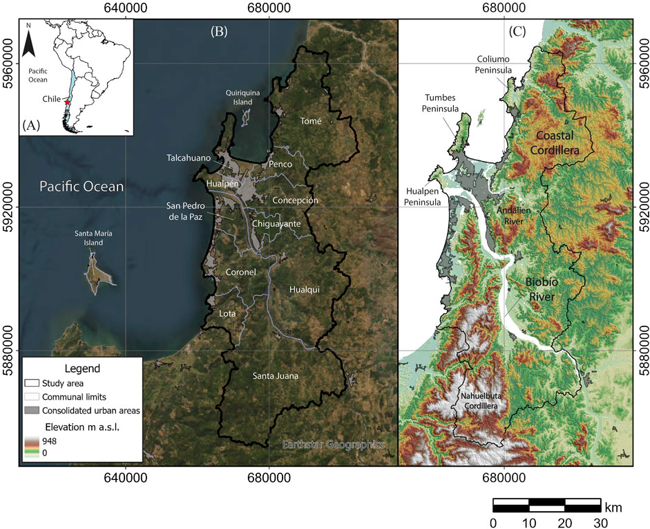
Figure 1. Location map of the Concepción Metropolitan Area (CMA). (A) South America and Chile. Red star indicates study area location; (B) Administrative divisions of the CMA in communes (municipalities); (C) Elevation map of the CMA. Legend and scale bar apply to (B, C).

Therefore, the goal of the research we report here was to construct a detailed landslide inventory in the Concepción Metropolitan Area, emphasizing a multitemporal, multi-source compilation, covering the period 1990 to 2023. We assessed our inventory relative to records from the Chilean Geological Survey (SERNAGEOMIN) and then performed a landslide susceptibility assessment to demonstrate the potential of our inventory approach.

2 Materials and methods

2.1 Study area

The CMA is in the Biobio Region, South-Central Chile, corresponding to the third largest urban area in Chile with a total population of over 1 million (INE, 2017). The CMA includes 11 municipalities or communes, covering 2,850 km² (Figure 1). This area is undergoing rapid urban growth due to rural-urban migration (Prada-Trigo et al., 2022), leading to expansion into areas with yet unknown landslide dynamics.

From a geological-geomorphological perspective, the CMA corresponds combines coastal, fluvial, and tectonic dynamics, confined between the Pacific Ocean and the western slope of the Coastal Cordillera, reaching elevations of over 300 m a.s.l. (Figure 1). A system of horsts and grabens developed in the Coliumo, Tumbes, and Hualpén Peninsulas (130, 160, and 200 m a.s.l. respectively) rise above the coastal areas and the emerged delta of the Andalién and Biobío rivers, evidencing tectonic blocks-oriented NE-SW (Mardones, 1978). Within the emerged delta, there are several inselbergs with heights exceeding 70 m a.s.l. All these elevated terrains have slopes averaging between 30° and 50°, developing steep scarps and slope valleys. These landforms are the result of tectonic activity from the subduction between the Nazca and South American plates, which has caused the uplift of Paleozoic metamorphic and granitoid rocks that constitute the basement of the study area, overlain by Triassic to Neogene continental and marine sedimentary rocks and unconsolidated Quaternary deposits (see Lithology in Figure 3G).

The climate of the CMA is mediterranean with warm, dry summers and cold, wet winters (Sarricolea et al., 2016). The average annual temperature is 12.4°C, 11.6°C in winter and 18.2°C in summer, and the total annual precipitation is around 1,000 mm, 70% concentrated between May and August (DMC, 2023). Extreme events records indicate that the coldest temperature was −3.8°C in July 1972 and 1976, and the warmest temperature was 34.4°C in February 2023. In the case of extreme precipitation records, the most significant pluviometric event in 24 h occurred on 26 June 2005, with an accumulation of 162.2 mm. These records also highlight the rainiest years with more than 1,500 mm in 1966, 1977 and 1997. While recent studies document an overall decrease in precipitation in south-central Chile (e.g., Garreaud et al., 2019), they also find a trend toward the concentration of precipitation into fewer events (Sarricolea et al., 2019).

2.2 Data for landslide events

We compiled data from 1990 to 2023 from various sources to generate the CMA Landslide Inventory. Figure 2 summarizes the methodological framework of this study. The initial historical data for landslide occurrences were collected from the Landslide cadastre of the Chilean Geological Survey (SERNAGEOMIN), available from the ITREND platform (https://www.plataformadedatos.cl/). The SERNAGEOMIN database for landslides contains events within the country until 2021. It is important to note that most of these records report approximate locations of the technical observation, rather than the specific landslide sites (Jorquera-Flores and González-Campos, 2024). In this study, we labelled these records as RAW-SNGM Landslide Inventory. For information from 2022 to 2023, we also consulted technical reports from the SERNAGEOMIN Library Website (https://catalogobiblioteca.sernageomin.cl/) and the technical minutes viewer for meteorological events (https://experience.arcgis.com/template/38dbe7203f314d22b8392953c056f16c). Given that many of these records contain approximate locations, many show unrealistic locations, such as on flat urban areas or along flat sections of main roads, rather than on the hillslopes associated with the landslide events. Using these locations provides inaccurate characterization of relevant factors, such as lithology and slope. Consequently, we reviewed all technical reports listed in these sources to determine the exact locations, adding them to the database. The corrected coordinate locations in this database correspond to the scarp centroid of each landslide event, labeling this dataset as SNGM Landslide Inventory.

Figure 2

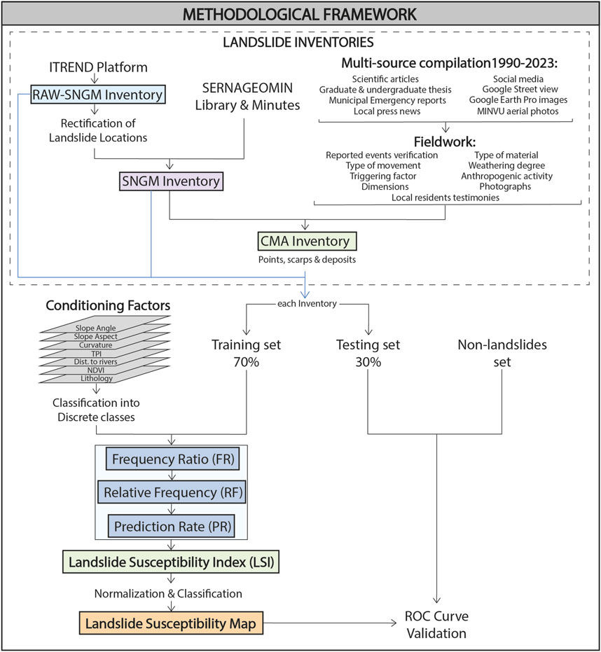
Figure 2. Methodological framework of the study.

Additionally, we compiled information from available scientific articles, graduate and undergraduate theses, and municipal emergency offices for the period 2022–2023. Records were also generated via analyzing local news reports from 1990 to 2023. Another source of records was social media platforms (Facebook, Instagram, and X/Twitter), where community-shared data were filtered using keywords in Spanish such as “derrumbe”, “deslizamiento”, “socavón”, “caída” and “aluvión”. These local reports provided information on location, occurrence date, affected infrastructure or people, triggering factors, and, in some cases, the type of movement. We supplemented this by checking some routes in Google Street View images, and with interpretation of Google Earth Pro images and aerial photos available from the Ministry of Housing and Urban Development of Chile.

We conducted extensive fieldwork across the CMA in 2022 and 2023 to verify and validate compiled records and to document new landslides in the surrounding areas that had not been previously reported. Our identification criteria applied a minimum threshold of 3 × 3 m; areas below this size were excluded from the inventory. We also categorized the type of movement and described the landslide components, following Cruden and Varnes (1996) and Soeters and van Westen (1996) guidelines. Detailed observations included triggering factors, failure surface shape, material type, presence and type of discontinuities, degree of weathering, activity degree, water content, drainage conditions, affected infrastructure and/or populations, and associated anthropogenic activities, and a photograph of the deposit, among other relevant factors.

For recent landslides, younger than six months, cleared vegetation is typically a key identification feature. However, vegetation tends to regenerate quickly, making it more challenging to identify certain characteristics, thereby affecting the accuracy of descriptions for older events. This limitation is also relevant when validating older records, particularly those predating 2010. To partially compensate for this effect, we relied on testimonies from local residents for validation, as shown in the flowchart of Figure 2.

2.3 Inventory fields

Our landslide inventorying closely follows guidelines from the protocol for Inventory Mapping of Landslide Deposits by Burns and Madin (2009) in terms of database structure within a Geographic Information System (GIS), adapting the spatial resolution according to the available imagery resources for the study area. Thus, the CMA Inventory is mainly a GIS database of points with an attribute table that, when possible, includes polygons describing scarps and deposits areas of a given landslide, created in shapefile format in ArcGIS Pro software. Landslide polygons were delineated only when the affected area spanned at least six pixels of the 5 m resolution LiDAR-derived Digital Terrain Model (DTM; see Table 2). Events smaller than this threshold were recorded as point features. The landslide inventory map is presented at a scale of 1:10,000, in accordance with guidelines for local mapping (e.g., Fell et al., 2008; van Westen et al., 2008).

The attribute table contains some fields from GEOMIN Portal database (https://portalgeominbeta.sernageomin.cl/), complemented by other relevant attributes indicated in Table 1, including location, date of occurrence, type of movements, causal factors, damage caused, among others (e.g., van Westen et al., 2008; Fell et al., 2008; Guzzetti et al., 2012; Tyagi et al., 2022).

Table 1

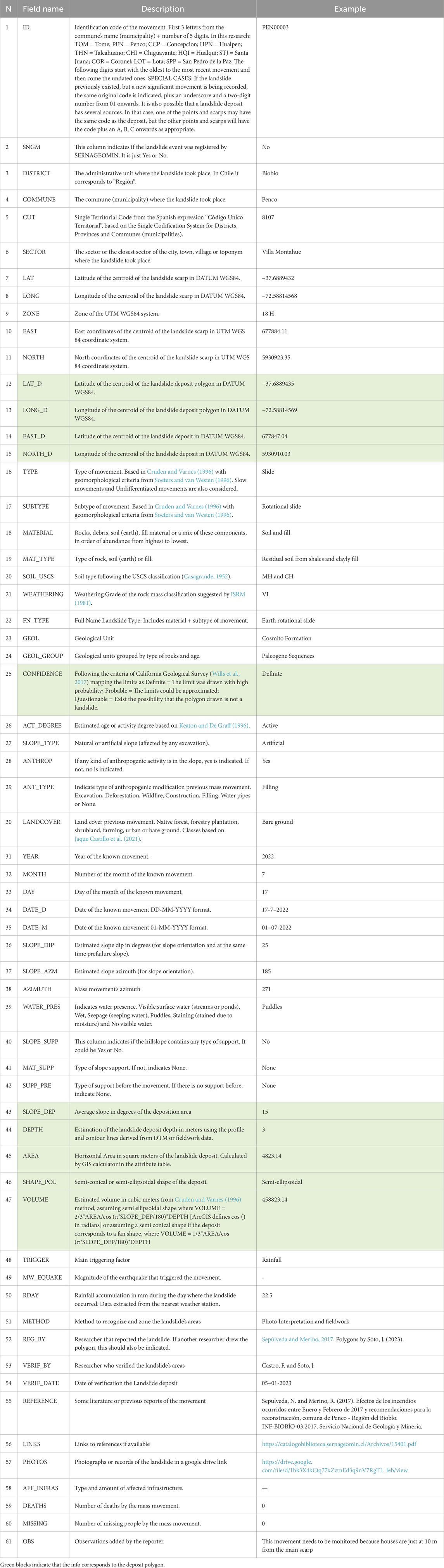
Table 1. Data fields for CMA Landslide Inventory.

We performed a descriptive analysis of these data to study their patterns and differences between SNGM and CMA inventories, while RAW-SNGM was excluded because the aim of generating this inventory is susceptibility analysis. This includes plots for each field category and density maps using the Kernel density tool in ArcGIS Pro software to represent spatial patterns, highlighting areas of high and low landslide concentrations to identify hotspots and spatial patterns. Records from Quiriquina and Santa María Islands were excluded, as these islands have low population density, and they are situated in different geological and geomorphological contexts from the mainland.

2.4 Landslide conditioning factors

Our inventory included seven conditioning factors widely used in the literature. Four of these factors correspond to elevation derivatives: Slope angle, Slope aspect, Curvature and the Topographic Position Index (TPI). We also considered the Distance to rivers, NDVI and Lithology (Figure 2). These are widely used causal factors for Landslide Susceptibility Assessment (van Westen et al., 2008; Reichenbach et al., 2018; Broquet et al., 2024). All the sources of these factors are indicated in Table 2. For the Susceptibility Assessment (see section 2.5) we used a 5 × 5 m grid resolution, so the layers were resampled, snapped and masked using the same Digital Terrain Model (DTM) raster in ArcGIS Pro. Figure 3 shows the display of each of the conditioning factors used in this study.

Table 2

Table 2. Conditioning factors sources for Landslide Susceptibility.

Figure 3

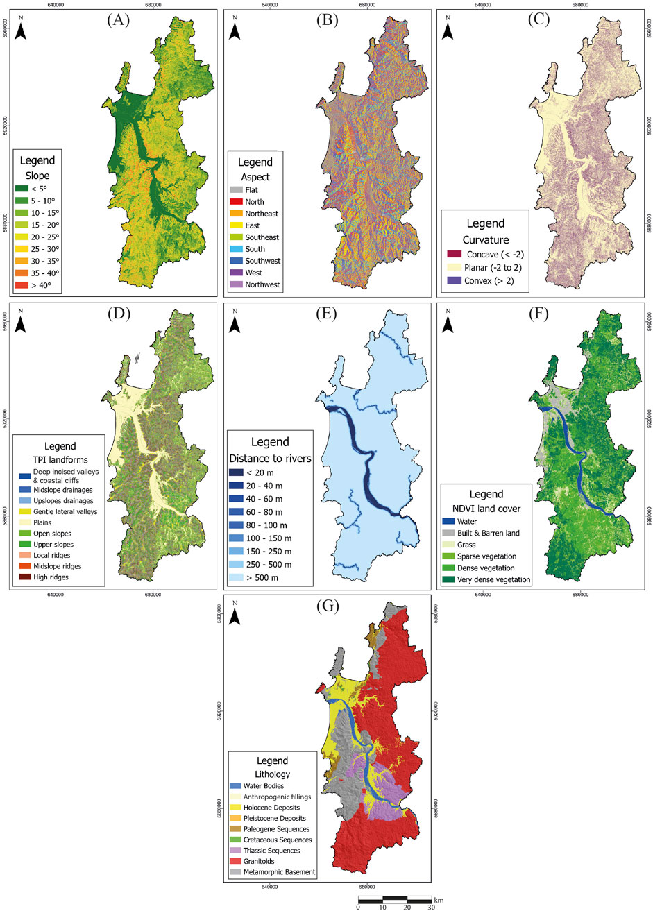
Figure 3. Landslide Conditioning Factors for the Susceptibility Assessment. (A) Slope angle; (B) Slope aspect; (C) Curvature; (D) TPI Landforms; (E) Distance to rivers; (F) NDVI land cover; and (G) Lithology. Scale bar applies to all factors.

The Slope Angle directly affects the gravitational force acting on a slope, which in turn influences the shear stress on the slope material. As the slope angle increases, the component of gravitational force parallel to the slope also increases, making the material more susceptible to failure (Keller, 2012; Brain and Rosser, 2022). Slope Aspect influences microclimatic conditions, such as incoming solar radiation, wind exposure, and precipitation patterns with north-facing slopes tend to receive more sunlight, becoming drier, while south-facing slopes retain more moisture (Méndez-Toribio et al., 2016; Pham et al., 2017). Curvature is also important for landslide susceptibility because it provides insights into the shape of the land surface, which influences how water flows and accumulates. This factor is described by combining the profile curvature and the planar curvature. Positive curvature indicates the slope is convex-up, negative indicates concave-up, and zero means flat. These different shapes affect water flows and accumulation, soil saturation and erosion (Pham et al., 2017; Alqadhi et al., 2022). These elevation derivatives were calculated with the tool “Slope”, “Aspect” and “Curvature” in ArcGIS Pro 3.2.2, respectively, from the 5 × 5 m LiDAR-derived DTM of the Ministry of Housing and Urban Development of Chile (Table 2).

The Topographic Position Index (TPI) following Weiss’ (2001), is an index that compares the elevation of each DTM pixel to the mean elevation of a circular neighborhood around it. Positive TPI values identify pixels that are higher than the average of their neighborhood; negative values indicate the opposite (Parra et al., 2021). The topographic position affects different processes in the landscape such as soil formation, microclimate conditions, moisture availability, among others (Méndez-Toribio et al., 2016). We classified the TPI values into 10 discrete landform classes by averaging over two neighborhoods within a radius of 100 and 1,000 m each using the TPI-Based Landform Classification from the SAGA GIS 7.8.2 toolkit in the QGIS software. These TPI Landforms are interpreted as geomorphic units within study area.

Distance to rivers is related to soil saturation, erosion rates, and riverbank stability. Proximity to rivers increases the likelihood of slope failure due to elevated groundwater levels and the undercutting of slopes by flowing water. Therefore, areas closer to rivers are susceptible to landslides (Pham et al., 2017). This parameter was calculated using the “Euclidean distance” tool in ArcGIS Pro 3.2.2 software from rivers indicated into the Base cartography from Ministry of Housing and Urban Development of Chile.

The stabilizing effect of vegetation on slopes is characterized via the Normalized Difference Vegetation Index (NDVI). Higher NDVI values indicate denser vegetation, which can reduce the risk of landslides by reinforcing soil structure and reducing surface erosion. Conversely, low NDVI values are indicative sparse vegetation or bare ground, increasing the likelihood of slope instability (Varnes, 1984; Doan et al., 2023). We computed the average NDVI from March 2017 to August 2024 using Sentinel 2 available data in Google Earth Engine (Table 2). We classified NDVI into six land cover classes following a modification of Doan et al. (2023) classes: Water (<−0.042), Built & Barren land (−0.042 – 0.182), Grass (0.182–0.327), Sparse Vegetation (0.327–0.425), Dense Vegetation (0.425–0.503) and Very Dense Vegetation (>0.503).

Lithology is also important because the type and characteristics of the rocks and their derived soil materials directly influence slope stability. Certain lithologies, such as highly weathered or fractured rocks, unconsolidated sediments and clay-rich soils derived from these rocks are prone to landslides due to their lower shear strength and higher susceptibility to water infiltration (Varnes, 1984; Cruden and Varnes, 1996; Keller, 2012). We incorporated this factor via compilation and reanalysis of several sources: available regional and detailed geological maps (e.g., Quinzio et al., 2011; Earth Sciences Department–UdeC, 2012; Earth Sciences Department–UdeC, 2015; Earth Sciences Department–UdeC, 2016; Earth Sciences Department–UdeC, 2018; Earth Sciences Department–UdeC, 2021; Molina, 2017; Rodríguez, 2022; Tomé Municipality, 2022) were scanned and digitized in ArcGIS Pro, and refinement/correction was undertaken in the field. We grouped units by their age and rock type, as they share some characteristics, weathering, degree of consolidation and soil properties. In general, the Metamorphic Basement corresponds to two series of Paleozoic metamorphic complexes (Eastern and Western Metamorphic Complexes) consisting of foliated phyllites and schists; the Granitoids correspond mainly to the Concepción Intrusive Complex and the Hualpén Monzogranite; Triassic sequences correspond to Santa Juana Formation, which consists mainly of continental conglomerates, sandstones and shales; Cretaceous sequences correspond to Quiriquina Formation, which consists mainly of fossiliferous marine glauconitic sandstones; Paleogene sequences correspond to Curanilahue and Cosmito Formations, which consist of continental shales and sandstones with some vegetal fossils and important coal layers; Pleistocene deposits correspond mainly to Andalién Formation and Molino El Sol strata, which are not well consolidated conglomerates and siliceous sandstones; Holocene deposits correspond to old and current coastal and fluvial deposits; and the Anthropogenic fillings correspond to non-consolidated old coal mine material.

2.5 Landslide susceptibility mapping

To test the potential of our inventory, we utilized it to carry out a susceptibility mapping, using the Frequency Ratio (FR) method, a bivariate statistical model, widely used in landslide susceptibility assessments due to its simplicity, straightforward computation, and its multi-scale scope, from global to local (Sujatha and Sudharsan, 2024). However, the method is bivariate, which makes it potentially sensitive to collinearity between variables (Nandi and Shakoor, 2010). To minimize this effect, we carefully selected a set of conditioning factors designed to avoid collinearity and ensure the reliability of the analysis. To apply the FR method, each conditioning factor must be classified into discrete classes. The classification breakpoints for each factor are detailed in Supplementary Tables S1–5. A summary of the method’s steps is provided in Figure 2. FR is calculated as follows:

$FR=\frac{\frac{L_i}{L_{tot}}}{\frac{X_i}{X_{tot}}}(1)$

where, FR is the frequency ratio of class i of a given conditioning factor X; L_i is the number of landslide pixels within class i; L_tot is the total number of landslide pixels; X_i is the number of pixels of class i of that given conditioning factor X; and X_tot is the total number of pixels of the conditioning factor X (all categories). The FR of each conditioning factor is merged via normalization values to a relative frequency (from 0 to 1) as follows:

$RF=\frac{{FR}_i}{{FR}_{tot}}(2)$

where RF corresponds to the relative frequency of each i class of the factor X; FR_i is the frequency ratio of class i of factor X calculated in Equation 1; and FR_tot is the sum (total) of frequency ratios of all classes of the factor X. After this normalization, RF becomes an indicator of the weight of the classes of each parameter but still considers all factors with the same weight (Acharya and Lee, 2019; Bammou et al., 2023). To solve this problem and to consider the mutual interrelationship between variables, the Prediction Rate is calculated as follows:

$\mathit{PR}=\frac{\left({RF}_{\mathit{max}}-{RF}_{\mathit{min}}\right)}{{\left({RF}_{\mathit{max}}-{RF}_{\mathit{min}}\right)}_{\mathit{min}\_all}}(3)$

where PR is the prediction rate of the parameter X; RF_max is the maximum value of relative frequency (RF) among all classes of parameter X calculated with Equation 2; RF_min is the minimum value of relative frequency (RF) among all classes of parameter X calculated with Equation 2; and the expression (RF_max–RF_min)_{min_all} is the minimum value of the differences between the maximum and minimum RF values of all parameters. FR and RF values of each class and PR of each conditioning factor calculated in this study are indicated in Supplementary Tables S1–5. Thus, the final step is to calculate the Landslide Susceptibility Index as a simple linear equation:

$LSI={\displaystyle \sum _{i=1}^n}{\mathit{PR}}_i*{RF}_i(4)$

where LSI is the Landslide Susceptibility Index; n is the number of conditioning factors used to calculate the index; PR_i is the prediction rate of the factor i obtained from Equation 3; and RF_i is the reclassified layer of the factor i assigning to each class its own relative frequency calculated with Equation 2. The LSI value obtained from Equation 4 was then normalized (LSI_norm) by scaling between the minimum (min) and maximum (max) values to achieve a range from 0 to 1:

${LSI}_{norm}=\frac{LSI-\mathit{min}}{\mathit{max}-\mathit{min}}(5)$

The LSI_norm obtained from Equation 5 was subsequently classified into five categories in order to generate the Landslide Susceptibility Map: Very Low (0–0.1), Low (0.1–0.2), Moderate (0.2–0.3), High (0.3–0.5), and Very High (0.5–1.0). We conducted this susceptibility analysis using three distinct datasets. First, we applied the analysis to the raw data from the ITREND platform (RAW-SNGM model). Next, we used the rectified data provided by SERNAGEOMIN (SNGM model). Finally, we analyzed using the newly generated inventory (CMA model). In the case of these Susceptibility Assessments, we did not consider Quiriquina and Santa María Islands records as these islands have different geological and geomorphological conditions from the mainland.

2.6 Landslide susceptibility validation

Validation of the Landslide Susceptibility model was carried out using the Receiver Operating Characteristic (ROC) curve and the Area Under the ROC Curve (AUC), which are widely accepted metrics for evaluating landslide model performance (e.g., Corsini and Mulas, 2017; Pham et al., 2017; Acharya and Lee, 2019; Alqhadhi et al., 2022; Bammou et al., 2023). First, susceptibility values were sampled from the susceptibility raster for both landslide and non-landslide points, as indicated in Figure 2. This resulted in two distinct datasets, one containing values for actual landslide locations (inventory) and the other for non-landslide areas. Non-landslide points were randomly selected across the study area, with each location manually verified to ensure the absence of recorded landslide events.

To quantify the model’s ability to distinguish between landslide-prone and non-landslide areas, the extracted values were combined into a binary-labelled dataset: 1 for landslide and 0 for non-landslide. Using the ROCR package in the R programming language (Sing et al., 2005; ROCR package version 1.0-11, 2020), these data were fed into a prediction object, which computed the true positive rate (TPR) and false positive rate (FPR) across various threshold values, forming the basis of the ROC curve. This ROC curve visually represents the trade-off between sensitivity (TPR) and the false positive rate (FPR; also known as 1 - Specificity). These values were calculated as follows:

$TPR=\frac{TP}{TP+FN}(6)$

$FPR=\frac{FP}{FP+TN}(7)$

where TPR is the True Positive Rate (Sensitivity); TP are the True Positives values; FN are the False Negative values; FPR is the False Positive Rate (1 – Specificity); FP are the False Positive values; and TN are the True Negative values.

Subsequently, the AUC value was computed from the ROC curve to summarize the overall performance of the susceptibility model as follows:

$AUC={\displaystyle \underset{0}{\overset{1}{\int }}}TPR\left(FPR\right)d\left(FPR\right)(8)$

where AUC is the integral of the ROC curve, which represents the plot of TPR versus FPR (obtained with Equations 6, 7) across different threshold values. The AUC calculated with Equation 8 provides a measure of how well the model distinguishes between landslide-prone and stable areas. This represents the probability that the model will rank a randomly chosen landslide-prone area higher than a randomly chosen non-landslide area. A value of 0.5 represents random guessing, while a value closer to 1 indicates excellent performance (Jiao et al., 2019). These AUC values are useful for comparing model performance.

3 Results

3.1 CMA landslide inventory

Our inventory contains 1,288 landslide records for the Concepción Metropolitan Area (CMA); we use 1,240 in the analysis presented in this section. The remaining 48 events are located on Quiriquina and Santa María Islands. The spatial distribution of these landslides is depicted in Figure 4A, showing many events occurring within or near urban areas, affecting houses and roads (Figure 4B). Figure 4C highlights key attributes from the CMA Inventory database. Each landslide record includes the type of movement, the geological unit group where the event occurred, coordinates, and the administrative division (municipality) where the landslide took place. Several fields are nearly complete, detailing slope type, associated anthropogenic activity (if present), and degree of activity. Notably, approximately 80% of the records specify the landslide’s triggering factor. Additionally, for the study area, it is significant that half of the recorded landslide processes include mapped deposit areas (Figure 4B), the date of occurrence, and information on slope supporting methods.

Figure 4

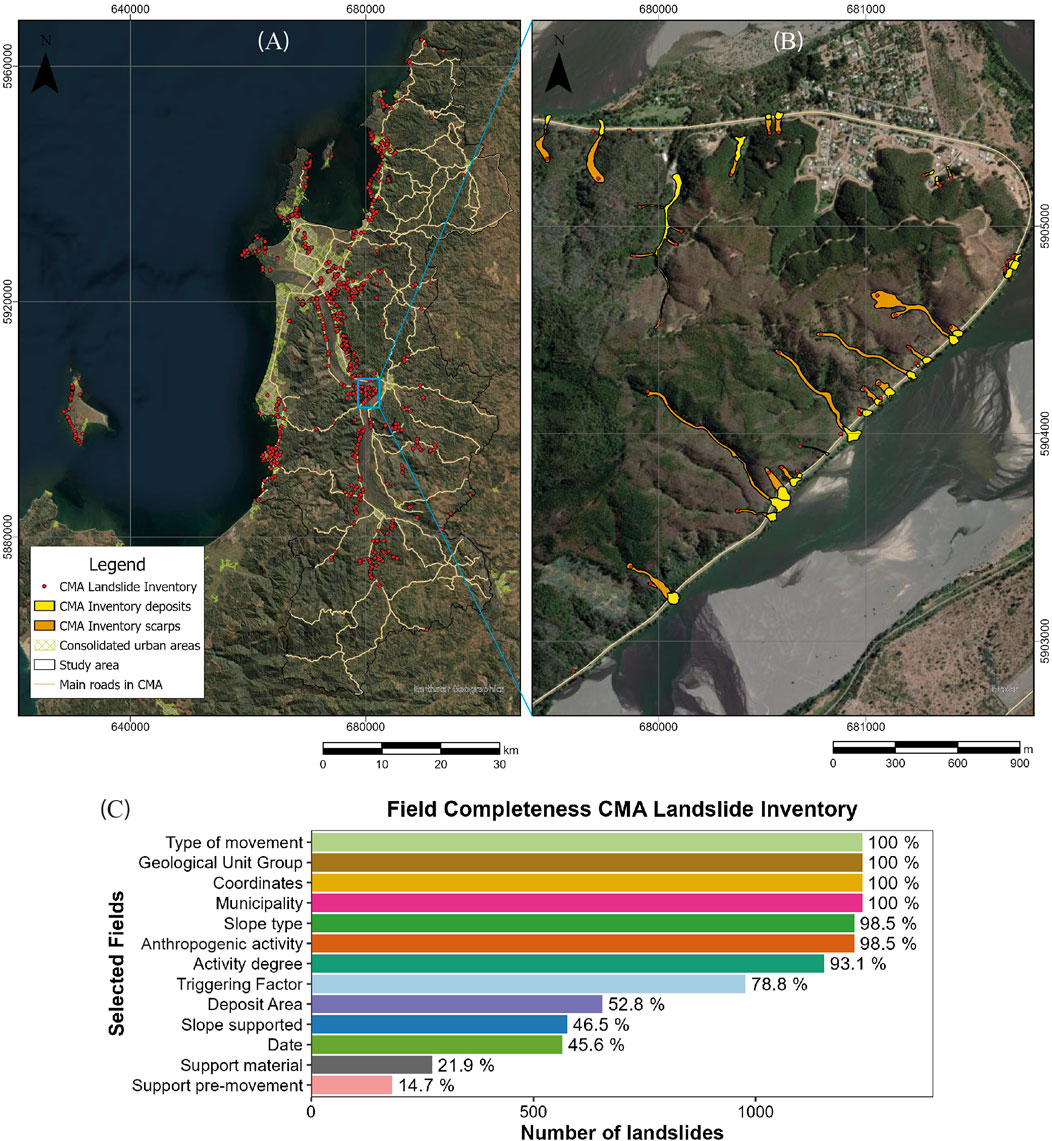
Figure 4. CMA Landslide Inventory locations and data. (A) Location of each landslide event in the study area; (B) A detailed view of an example location in (A); (C) Selected fields of the inventory database and their percentage of completeness.

3.2 CMA and SNGM landslide inventories comparison

Figures 5A, B illustrate the spatial distribution of landslide records using density mapping for the SNGM and CMA inventories, respectively. Between 1990 and 2023, the SNGM inventory records 159 events, while the CMA 1,240. Although both inventories overlap in certain areas, particularly within urban zones, the CMA inventory provides a denser and more comprehensive coverage, identifying new landslide-prone zones, such as the northern coastal parts of Tomé, the coastline between Tomé and Penco, additional points in the Hualpén Peninsula, Hualqui and Santa Juana.

Figure 5

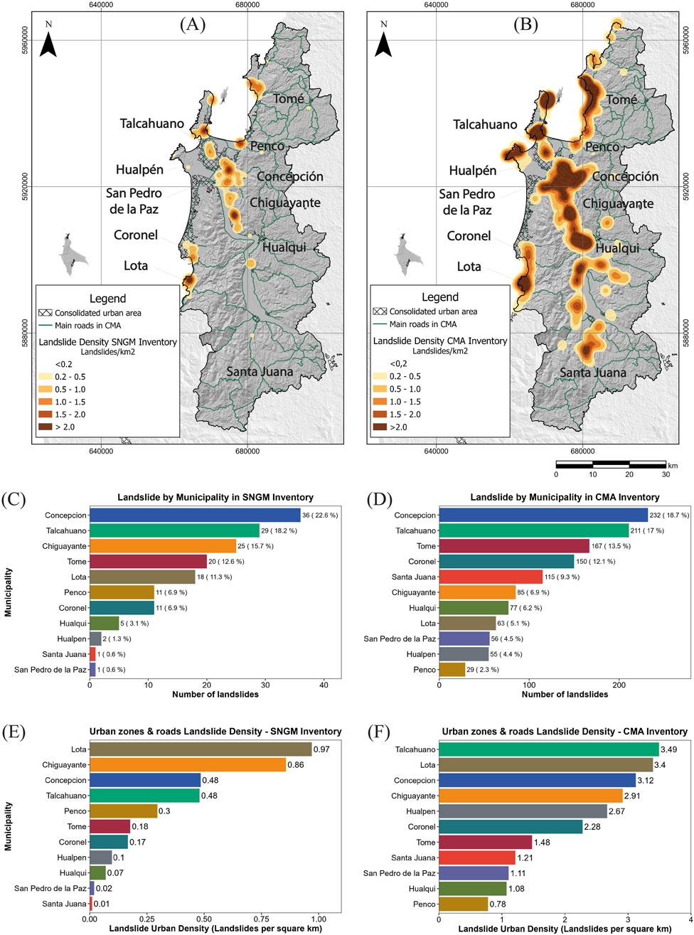
Figure 5. Landslide Density Maps. (A) SNGM dataset; (B) CMA dataset; (C, D) show the amount of landslide records in each municipality; (E, F) indicate landslide records inside a buffer of 500-m from urban zones and 100-m of from roads to represent affected urban areas and main roads.

Observing the distribution of landslide events by municipality (Figures 5C, D) reveals notable differences, particularly in San Pedro de la Paz, Santa Juana, Hualpén, and Hualqui. In these areas, the SNGM inventory records fewer than five events per municipality, whereas the CMA reports more than 50.

Differences in landslide density between the two inventories are evident. Figures 5E, F display the density of records within a 500-meter buffer of urban zones and a 100-m buffer of main roads. In the SNGM inventory, Lota is the most affected urban area and Santa Juana the least. Conversely, in the CMA inventory, Talcahuano is the most affected, while Penco is the least impacted by landslides near urban areas and main roads. These discrepancies highlight the broader and more detailed scope of the CMA inventory, which captures a more accurate picture of landslide occurrence in the region. Talcahuano and Lota are particularly critical municipalities in terms of landslide density, especially in urban zones and along major roads that could be impacted.

In terms of geological units, according to the SNGM inventory most of the records are concentrated in Paleogene sequences, followed by Granitoids and Metamorphic basement (Figure 6A). However, when we superimpose our geological unit map (Figure 3G) and this inventory, via normalization between number of records and unit area the result is different, with Pleistocene deposits, Cretaceous sequences and Paleogene sequences as the most landslide-prone units (Figure 6C). On the other hand, for the CMA inventory most of the records are concentrated in the Metamorphic basement and Granitoids, then Paleogene sequences (Figure 6B), but when analyzed by spatial surface area of the geological unit group, Cretaceous sequences, Anthropogenic fillings and Pleistocene deposits are indicated as the most landslide-prone units (Figure 6D). The CMA inventory contains four new landslide records in anthropogenic fillings consisting of unconsolidated material from uninhabited old coal mining operations in Lota.

Figure 6

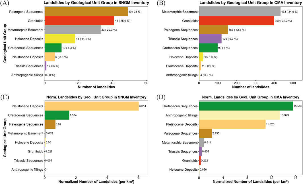
Figure 6. Landslide distribution by Lithology (geological unit groups). (A, B) Number of landslides in each geological unit group in SNGM and CMA inventories respectively; (C, D) Normalized number of landslides by geological unit group surface in square kilometers in SNGM and CMA inventories respectively.

In the SNGM inventory, slides account for more than 70% of events, followed by lateral spreads, falls, and flows, each with fewer than 20 recorded events (Figure 7A). Similarly, Figure 7C reveals that in the CMA inventory, slides records are also more than 70%, with flows and falls exceeding 100 records each. Regarding triggering factors, Figure 7B indicates that in the SNGM inventory, 60% of slides are rainfall-induced, with the remainder triggered by earthquakes and a small portion by anthropogenic activity. Flows and complex movements in this inventory are predominantly triggered by rainfall, while falls and lateral spreads are mainly earthquake-induced. Notably, there are no records of topples or slow movements in this inventory. Conversely, Figure 7D shows a wider range of triggering factors in the CMA inventory, with 90% of landslides being rainfall-triggered, followed by those caused by earthquakes, anthropogenic activity, and wildfires. Flows and complex movements are likewise driven by rainfall. Lateral spreads are mainly triggered by earthquakes, consistent with the SNGM inventory. However, in the CMA inventory, falls are primarily rainfall-induced (77%), with additional triggers including earthquakes, anthropogenic activity, coastal erosion, and wildfires. Topples are linked to anthropogenic activity and tree root growth (two records reported), while the triggering factor for slow movements remains unclear.

Figure 7

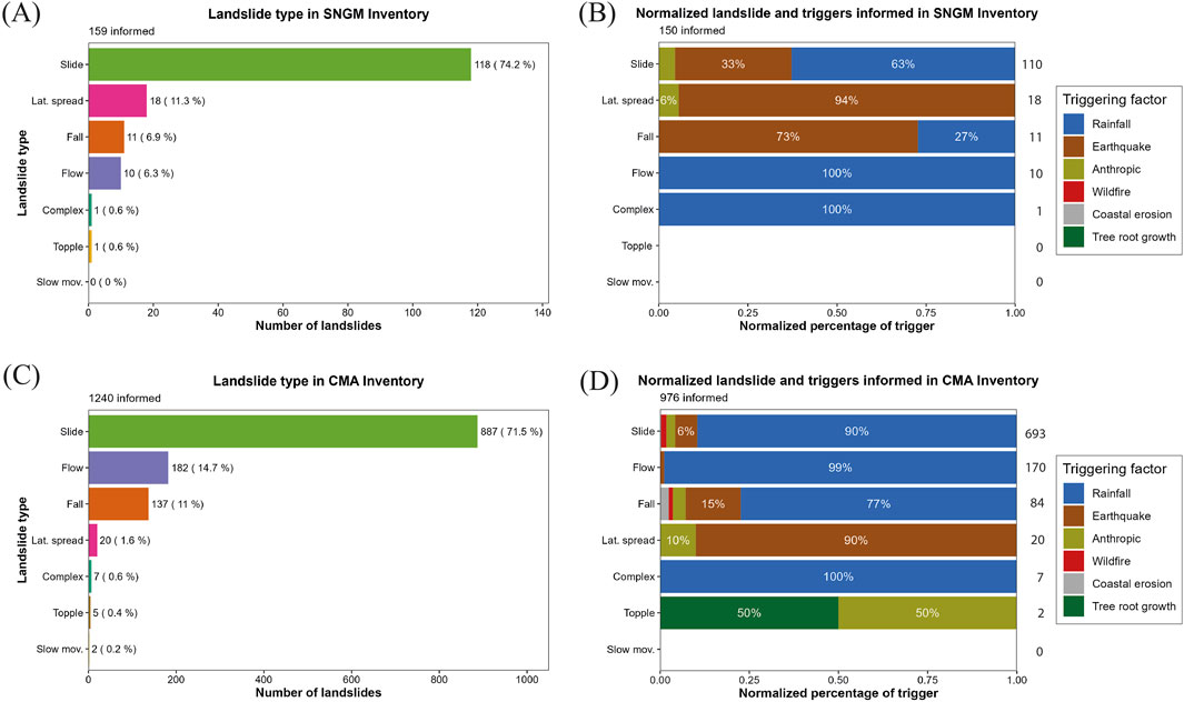
Figure 7. Landslide distribution by type and triggering factor. (A, C) Number of landslides in SNGM and CMA inventories respectively by type of movement; (B, D) Normalized number of landslides by type of movement in SNGM and CMA inventories respectively. Informed events in each bar indicated to the right.

Figures 8A, B present the monthly distribution of landslide occurrences in the SNGM and CMA inventories, respectively, while Figures 8C, D show the records arranged by year. The peak for earthquake-induced landslides in the SNGM inventory occurs in February, whereas rain-triggered events are concentrated between June and August (Figure 8A). In contrast, the CMA inventory reveals two significant peaks: February for earthquake-induced landslides, consistent with the SNGM inventory, while July for rainfall-triggered landslides (Figure 8B). The CMA inventory records landslides triggered by wildfires from December 2022 (see Figures 8B, D), primarily in Tomé, caused by the weakening of foliated metamorphic rocks of the Metamorphic basement and discontinuities in the Paleogene and Cretaceous sequences. The heat from the wildfire destroyed the root systems of large trees that had previously strengthened the rock mass, leading to landslides when the support was lost. The rainfall-triggered and wildfire-triggered landslide pattern are not identified in the SNGM inventory due the limited number or records.

Figure 8

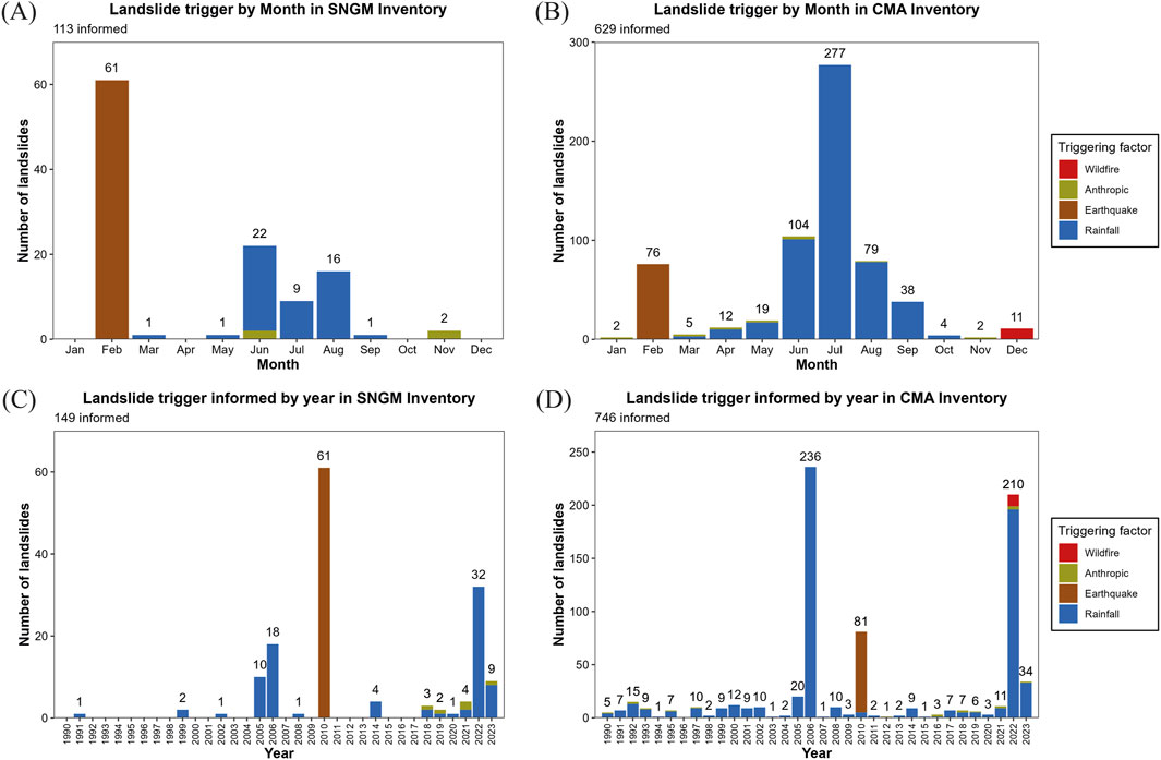
Figure 8. Landslide distribution by period. Number of landslides in SNGM and CMA inventories and their triggering factor respectively by month (A, B), and by year (C, D).

For the annual distribution, Figure 8C displays five notable peaks in the SNGM inventory, each with more than nine records. Four of these peaks, in 2005, 2006, 2022, and 2023, are predominantly associated with rain-induced landslides, while the most significant peak in 2010 corresponds to earthquake-triggered events. Similarly, Figure 8D for the CMA inventory identifies three significant peaks, occurring in 2006 and 2022, primarily due to rain-induced landslides, and in 2010, mainly by earthquake-induced events (also consistent with the SNGM inventory). SERNAGEOMIN technical reports indicate that on 26 June 2005, an intense storm that delivered 162.4 mm of rain in 24 h, triggering significant landslides in the study area (e.g., Naranjo S. et al., 2006). The SNGM inventory contains records of this storm, and the CMA inventory registers only 10 additional records related to this extreme weather event. Another significant rainfall event occurred in July 2006, with 164 mm falling over three days and 230 mm six days between July 5 and 11 (Naranjo J. et al., 2006). This event triggered several landslides that are included in the CMA inventory. The year 2010 has many records in both inventories, primarily due to the Maule Earthquake (Mw = 8.8; Mardones and Rojas, 2012; Serey et al., 2019), which impacted south-central Chile. Despite the region’s well-known history of seismicity, this is the only earthquake event that has significantly triggered landslides.

In 2022, both inventories contain many more landslide records relative to previous years. SERNAGEOMIN’s technical reports documented rainfall-induced events throughout the year. Considering precipitation data from the Carriel Sur meteorological gauge located between Talcahuano and Concepción (labelled as RDAY field in CMA inventory), significant events occurred on June 4–6, with at least 100 mm of rainfall accumulated over three to five days, followed by rain events throughout July. August 16 also stands out, following a 40 mm rainfall the previous day. This high volume of records in 2022 relative to previous years may reflect a recording bias, as the main fieldwork campaign was conducted in 2022 and early 2023. Additionally, in 2023 SERNAGEOMIN introduced technical minutes for more precise landslide registration. In the CMA inventory, were prominently recorded due to media and social media reports helped in recording many urban landslides. Two key rainfall events in 2023 were June 24, with nearly 100 mm of rain over four days, and a storm from August 15–24, bringing approximately 100 mm over ten days.

3.3 Spatio-temporal distribution of CMA landslide inventory

The CMA inventory was divided into five-year intervals to examine spatio-temporal patterns and recurrence (Figure 9). Within each time interval, certain spatial patterns emerge. For instance, the hillslopes of Concepción, Talcahuano and Chiguayante consistently show recurrent landslides in the same places. Records for Coronel, Lota, Penco, and Tomé localities become more consistent from 2005–2009 onwards (Figures 9D–G), while landslides in the Hualpén Peninsula only appear in the 2020–2023 interval (Figure 9G). Lastly, Hualqui and Santa Juana show more substantial records in 2005–2009 and 2020–2023 (Figures 9D, G), largely due to the addition of photointerpretation data in rural areas, which are significant in these municipalities. Indeed, an analysis of landslide density distribution over time reveals that the periods 1990–1994, 1995–1999, 2000–2004, and 2015–2019 contain approximately 30 landslide records each (Figure 9H). The years with the highest number of records are 2005–2009 and 2020–2023, largely explained by the rainfall and events mentioned earlier. This temporal breakdown highlights that different landslide types are distributed unevenly over time. Slides are consistently present throughout the entire study period. Flows show a substantial increase in 2005–2009, while falls are mainly recorded in 2010–2014 and 2020–2023. Lateral spreads were primarily recorded in 2010–2014, corresponding to the Maule Earthquake in 2010.

Figure 9

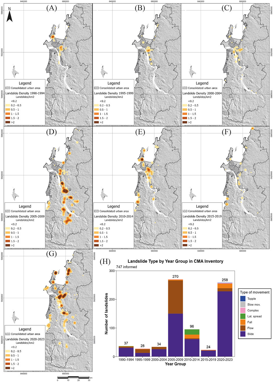
Figure 9. Landslide distribution by 5-year period. (A–G) Landslide density from 1990 to 2023 in 5-year subdivision; (H) Bar plot of landslide records by type of movement in this time subdivision.

3.4 Landslide susceptibility intercomparison

3.4.1 Slide susceptibility

Figure 10 illustrates the landslide susceptibility models based on the RAW-SNGM, SNGM, and CMA inventories. AUC values are 0.7035 for the RAW-SNGM model, 0.7986 for the SNGM model, and 0.8714 for the CMA model (Figure 10G). At the regional scale, the RAW-SNGM model indicates large areas of high susceptibility in flat urban zones, which are instead classified as low or very low susceptibility in both the SNGM and CMA models. Differences among models that are subtle at the regional scale become more pronounced at the local level. For example, Figures 10D–F show models’ results for the Lota area (RAW-SNGM, SNGM, and CMA, respectively), indicating overestimation of the RAW-SNGM model of areas classified as low or very low susceptibility in the SNGM and CMA models (Figures 10E, F). Notably, the CMA model weighs higher drainage lines and steep hillslopes with high slope angles, whereas the SNGM model reflects a generally more conservative susceptibility classification.

Figure 10

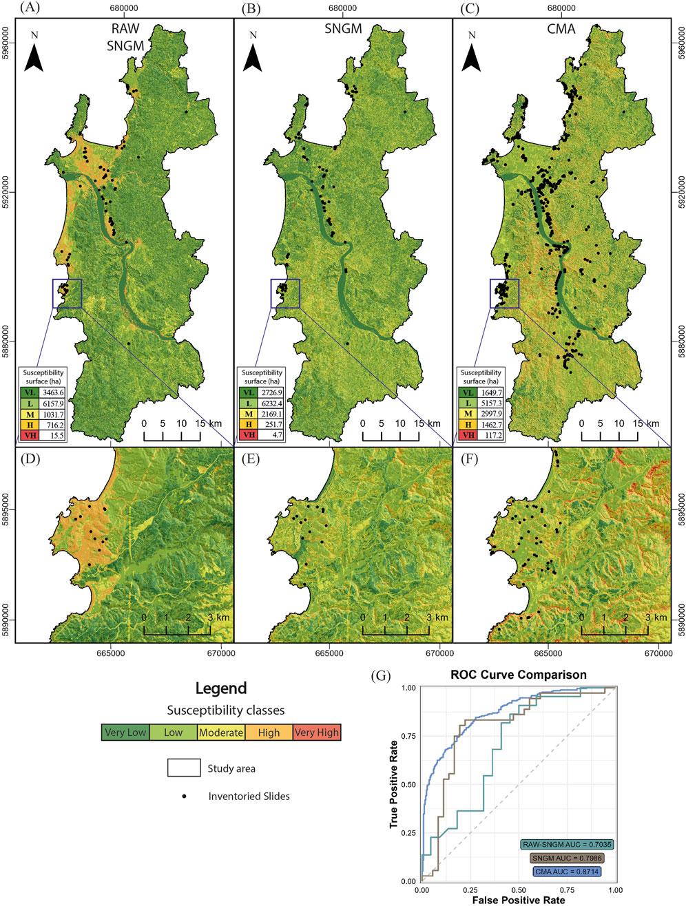
Figure 10. Slide Susceptibility Maps. (A) RAW-SNGM Slide Model for the study area; (B) SNGM Slide Model for the study area; (C) CMA Slide Model for the study area; (D), (E, F) RAW-SNGM, SNGM and CMA models for Lota area respectively; (G) ROC Curve for the models’ performances. Blue rectangles in (A), (B, C) indicate (D), (E, F) locations. Legend represents elements of (A–F). VL, L, M, H and VH in (A) to (C) indicates classes Very Low, Low, Moderate, High and Very High respectively.

The differences between these slide models stem from the Prediction Rate (PR) values associated with each conditioning factor, as presented in Table 3. Lithology emerges as a highly significant factor across all three models, with the strongest influence observed in the RAW-SNGM and SNGM models, where it ranks as the most impactful factor. In the CMA model, while Lithology remains important, it ranks as the second most influential factor after Slope Angle. The latter factor is also critical to all models, since it is the second most influential factor in the SNGM model. NDVI Land Cover underscores the role of vegetation as a predictor, especially in the RAW-SNGM model, where the class Built & Barren land accounts for over 50% of the relative frequency (RF) of landslide records (see Supplementary Table S1), leading to overestimations in urban areas due to uncorrected slide events. By contrast, Distance to Rivers and Curvature exert moderate influence, while Slope Aspect and TPI Landforms have minimal impact on susceptibility compared to other conditioning factors.

Table 3

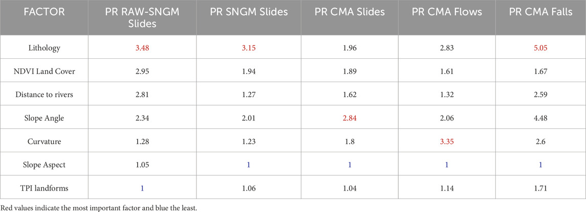
Table 3. Prediction rate of each conditioning factor for each model.

3.4.2 Flow and fall susceptibility

Figure 11A displays the CMA flow susceptibility model, which has an AUC of 0.8284. Figure 11C provides a closer view of the Chiguayante locality, an area well known for flow occurrences within the CMA (e.g., Mardones et al., 2004; Naranjo J. et al., 2006). Notably, major drainage channels along the hillslopes show high and very high susceptibility values for flows, with several records aligning with these areas, particularly near urban zones. This suggests increased risk of flows in proximity to inhabited areas.

Figure 11

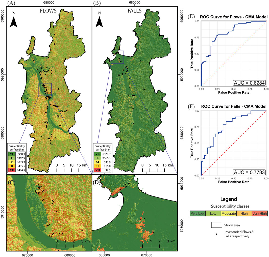
Figure 11. Flow and Fall Susceptibility for CMA. (A, B) Models for the whole study area; (C) Flow Susceptibility model for Chiguayante; (D) Fall Susceptibility model for Talcahuano; (E, F) ROC Curve for the models’ performances. Blue rectangles in (A, B) indicate (D, E) locations. Legend represents elements of (A–D). VL, L, M, H and VH in (A, B) indicate Very Low, Low, Moderate, High and Very High respectively.

Figure 11B presents the regional output of the CMA fall susceptibility model, with an AUC of 0.7783. Figure 11D highlights the Talcahuano locality, an area with numerous rockfall records in the CMA inventory database. Despite the model’s fair AUC value, there appears to be some overfitting, likely due to a significant bias in the distribution of the records. This bias seems to result from the high concentration of rockfall events within the Quiriquina Formation (Cretaceous Sequences), a geological unit with limited spatial extent. The model assigns high and very high susceptibility values to this unit, even though several rockfall records occur outside of it, indicating the model may overemphasize susceptibility in areas with a high density of records, regardless of the likely importance of other geomorphic factors.

4 Discussion

4.1 Landslide inventory standardization in Chile

Despite Chile’s high susceptibility to landslides due to its complex topography and active tectonics, the country still lacks a standardized national landslide inventory. The Chilean Geological Survey (SERNAGEOMIN) plays a critical role in providing essential information on geology, natural resources, and geological hazards, enabling Chile’s economic development and population welfare. The agency’s responsibilities extend beyond hazard management as it also offer valuable insights that aid economic planning and disaster preparedness. The involvement of SERNAGEOMIN in landslide assessments often begins with technical reports issued in response to national emergencies. Their focus is largely on post-disaster contexts, where resources are allocated to analyze and understand affected areas. The agency’s mandate extends beyond landslides, encompassing tsunamis, earthquakes, and volcanoes, and occasionally includes support for flood responses and wildfire recovery.

The landslide cadastre of the Chilean Geological Survey (SERNAGEOMIN), accessible through the GEOMIN Portal, functions primarily as a viewer for the general location of technical reports on landslide hazards, rather than as a detailed, comprehensive inventory of landslide events. This database provides approximate landslide locations and thus is unable to capture the full scope of landslide factors and occurrences across the country (Jorquera-Flores and González-Campos, 2024). Consequently, raw data from SERNAGEOMIN is of limited use for conducting detailed landslide assessments, as our analysis of the RAW-SNGM demonstrated. Additionally, the database is not regularly updated, missing recent information that is critical to conduct detailed assessments.

While several scientific studies have compiled landslide inventories across various regions of Chile, the lack of standardization in landslide data collection and reporting has resulted in a significant disparity of scales, identification protocols, and criteria on what kind of event is worth recording. For instance, Crosta et al. (2014) produced a polygon-based inventory of large landslides in major valleys of northern Chile. Serey et al. (2019) compiled a point-based inventory of earthquake-induced landslides triggered by the Maule Earthquake that occurred in 2010, focusing on lateral spreads, flows, disrupted slides, and coherent slides. Morales et al. (2021) developed a polygon-based temporal landslide inventory using machine learning for northern Chilean Patagonia, concentrating on slides, rockfalls, and debris flows. Subsequently, Morales et al. (2022) expanded this inventory using deep learning techniques, albeit without differentiating between landslide types.

Although these efforts have advanced the understanding of landslide distribution in Chile, there is no consensus on a standardized approach for inventorying landslides. A notable first step towards this was proposed by Jorquera-Flores and González-Campos (2024), who recommended the standardization of landslide databases in the Aysén region, located in southern Chile, improving the GEOMIN database field. Despite this, in Chile, an appropriate mapping scale has not been defined, given the diverse geographic and environmental contexts across the country. In our study, we built upon this work to generate a detailed, multitemporal landslide inventory that distinguishes between scarp and deposit areas as much as possible with the available resources, using both point and polygon data, following guidelines for local landslide hazard zoning at a scale of 1:10,000 recommended in the landslide literature (e.g., Fell et al., 2008; van Westen et al., 2008). This approach aims to provide detailed information for future analysis.

There are similarities between the database fields of Jorquera-Flores and González-Campos (2024) and the inventory presented in this study, such as the inclusion of a unique identification code for each landslide, date of occurrence, type of movement, type of material, coordinates and coordinate system, deposit area and volume, triggering factors, and references. However, there are key differences. For example, Jorquera-Flores and González-Campos (2024) presented a logic model for inventorying landslides and did not specify whether their data were point-based, polygon-based, or both, whereas our CMA inventory compiled landslide information and incorporated both types of data records depending on availability. Additionally, while both studies included rainfall as a triggering factor, our inventory only considered rain accumulation, whereas Jorquera-Flores and González-Campos (2024) also accounted for rainfall intensity and the gauge source of the data. Our inventory adds more detailed fields related to the material, such as the geological unit, geological unit group, type of material (distinguishing specific rock and soil types), and weathering conditions. We also incorporated information on anthropogenic activity, hillslope support systems for stabilization, water presence, and photographs of the landslide deposit when available.

4.2 SNGM and CMA landslide inventories comparison

Our CMA Inventory expands on what is available from the SERNAGEOMIN database (SNGM inventory), providing a more comprehensive spatial distribution of landslide records. It also adds significant new data in previously underrepresented areas, identifying landslides in locations largely overlooked by the SNGM inventory, such as Hualqui and Santa Juana. Although both inventories agree that urban areas and major roads in Talcahuano, Lota, Chiguayante, and Concepción have higher concentrations of landslide records, there are differences in the ranking of critical areas.

In turn, both the SNGM and CMA inventories agree that Pleistocene deposits and Paleogene sequences are particularly susceptible to landslides, and many of these deposits are found in residential areas, particularly northern parts of Concepción and the southern sector of Penco, where these deposits outcrop, consisting primarily of unconsolidated conglomerates from the Pleistocene deposits (Andalién Formation), sandstones and shales of the Paleogene Sequences (Cosmito Formation). On the other hand, CMA and SNGM inventories disagree on the impact of the Cretaceous Sequences (Quiriquina Formation) as a notably larger number of slides and rockfalls in the CMA inventory. This may have resulted from possible biases in documenting older slides and rockfalls (even pre-1990) along the coastal cliffs where the Quiriquina Formation outcrops. Although the sandstones of the Quiriquina Formation appear resistant, their numerous joints in multiple directions increase their susceptibility to these types of mass movement.

While the SNGM inventory provides a robust dataset for the quantitative analysis of slides, it lacks sufficient data for other movement types, such as flows, falls, and lateral spreads. Addressing this limitation requires qualitative or heuristic methods to develop susceptibility analyses. Given the size and level of detail of the CMA inventory, it is well-suited for the quantitative assessment of slides, flows, and falls. However, the analysis of lateral spreads, topples, complex movements, and slow movements remains a challenge due to the few available records for each of these landslide types. Therefore, future data collection efforts should focus on expanding the dataset for these underrepresented processes. For instance, recent efforts made at particular locations, such as the work of Fustos et al. (2017) on deformations of slow movements in Chiguayante during the winter of 2006, can be replicated across the entire area and integrated into the database. Therefore, while both inventories enable quantitative analysis of rainfall-induced slides, the detail of the CMA allows more comprehensive characterization as it provides descriptions of a range of landslides, including flows and falls. Nevertheless, conducting a quantitative assessment of earthquake-induced landslides remains challenging for both inventories due to limited availability of data on slides and falls.

The temporal distribution of landslides in the SNGM and CMA inventories reflects both seasonal and event-driven patterns. Notably, both inventories indicate peaks in landslides due to earthquakes and rainfall triggers, but they also reveal distinct differences based on data availability. Monthly patterns reflect the influence of seasonal factors, especially rainfall. Both inventories demonstrate a clear trend for rainfall-triggered landslides during the winter months (mainly June to August), with the CMA inventory showing a normal distribution with its peak in July, characteristic of Chile’s winter season. This aligns with the region’s rainfall patterns, where heavy and prolonged rainfall saturates the slopes and triggers landslides. In contrast, the February peak for earthquake-induced landslides, observed in both inventories, underscores the impact of the Maule Earthquake (Mw = 8.8; Mardones and Rojas, 2012; Serey et al., 2019).

Both inventories identified significant landslide peaks in specific years, primarily 2005, 2006, 2010, 2022, and 2023, each corresponding to either extreme rainfall events or the Maule Earthquake in 2010. The rainfall-triggered landslide peaks in 2005, 2006, and 2022 highlight the importance of threshold-based rainfall monitoring. Defining thresholds is crucial for developing early warning systems for communities in susceptible regions. Although the region typically experiences moderate seismicity, the Maule Earthquake triggered a significant number of landslides. Within the SNGM inventory, 52% of the landslides were rainfall-induced, whereas 38% were attributed to this seismic event. However, the CMA inventory shows a greater influence from rainfall, with 69% of its landslide records linked to rainfall events and only 6% related to the Maule Earthquake. These contrasting trends suggest that mitigation efforts should be tailored to address the predominant triggers in each inventory. For instance, slope stabilization measures may be particularly beneficial during the winter months, given the high proportion of rainfall-triggered landslides. In contrast, preparedness for earthquake-induced landslides should be a continuous priority, given the unpredictability of seismic events and their potential for widespread impact.

A key distinction between the SNGM and CMA inventories is their data completeness. The CMA inventory’s reliance on multiple data sources, including high-resolution satellite imagery, technical reports, and photointerpretation, allows for more comprehensive landslide documentation, especially rainfall-induced events that may not have been captured in the SNGM dataset. Additional sources in the CMA inventory have improved its resolution, highlighting landslides that might otherwise go unrecorded. This increased detail reveals the impact of data-collection biases. The influence of field campaign timing, especially the increased documentation in 2022–2023 in the CMA inventory, raises questions about temporal biases in landslide data collection. While these efforts have enriched the data, they may have overrepresented landslides during this period. This observation underscores the need for continuous and systematic data collection across seasons and years to enhance landslide monitoring and risk assessment accuracy.

Landslide recurrence revealed by the CMA inventory suggests underlying predisposing factors in particular areas, such as the geological structure, slope gradient, and land cover. Regular landslide activity in Concepción and Talcahuano may indicate the need for enhanced monitoring and preventative measures in these urban areas, especially given their population density and infrastructure. Additionally, the emergence of landslide records in municipalities such as Coronel, Lota, Penco, and Tomé after 2005 could reflect improved data-collection efforts. The increase in recorded landslides in rural regions, such as the Hualpén Peninsula, Hualqui, and Santa Juana, particularly in the latest interval (2020–2023), may be attributed to the expanded photointerpretation data. This increase suggests that landslides may have been historically underreported in these areas due to data limitations. Consequently, recent advances in data acquisition, particularly in rural settings, enhance our understanding of landslide distribution and suggest that comprehensive remote sensing data can reveal previously overlooked patterns. The recent identification of active landslide areas in rural regions suggests that these communities may also benefit from early warning systems and improved land-use planning.

Although landslide susceptibility analysis is generally not considered time-dependent, it is sensitive to the timing of landslide record acquisition (Jones et al., 2021). While a detailed susceptibility analysis for each time interval in the CMA inventory was not conducted, the variation in the number and spatial distribution of landslide records across time periods suggests that susceptibility results would differ accordingly. Thus, systematization and standardization of landslide inventorying need to incorporate protocols that account for the time-dependent evolution of these dynamics.

4.3 Slide susceptibility

Comparative analysis of landslide susceptibility models derived from the RAW-SNGM, SNGM, and CMA inventories revealed notable differences due to variations in inventory accuracy. The superior skill of the CMA model, according to AUC highlighting the impact of detailed inventories for landslide susceptibility assessments. The SNGM model also shows reasonable predictive capability as a result of rectified locations of the SERNAGEOMIN cadastre, The RAW-SNGM model, with the lowest AUC, overestimated susceptibility, particularly along urban areas that are known for their very low susceptibility to landslides. This overestimation reflects the influence of uncorrected landslide records, particularly in areas of flat urban terrain, where the CMA model classifies them as low or very low susceptibility.

Lithology is consistently a critical factor across all models, yet its influence is most pronounced in the RAW-SNGM and SNGM models, where it ranks as the leading conditioning factor, highlighting the role of rocks and derived soils in predisposing areas to landslides. In contrast, the CMA model assigns slightly lower importance to lithology, reflecting a more balanced integration of additional factors. Slope Angle also emerges as a critical predictor across models, particularly in the CMA model, underscoring the importance of steep terrain in landslide susceptibility. NDVI Land Cover, particularly the “Built & Barren land” class, contributed significantly to susceptibility in the RAW-SNGM model, indicating that urban and sparsely vegetated areas are associated with high susceptibility. However, the influence of this factor appeared less pronounced in the SNGM and CMA models, suggesting that curated inventories have adjusted for potential biases in urban areas, where landslide susceptibility may have been overstated.

Our findings point to the key positive impact of comprehensive, corrected inventories in the development of robust landslide susceptibility models, facilitating accurate and localized susceptibility assessments, which are indispensable for risk-informed planning and development in regions prone to landslides. On the other hand, relying on less accurate inventories, such as the RAW-SNGM, may result in unnecessary construction restrictions in stable areas, leading to economic losses, reduced development opportunities, and inflated property costs, ultimately hindering urban expansion and impeding community growth.

Earlier studies, such as those by SERNAGEOMIN (2012), conducted preliminary hazard assessments for the Biobio region (including the CMA) using heuristic susceptibility assessments. SERNAGEOMIN approach measured spatial relative probability alone rather than spatial and temporal probability; thus, it did not meet the requirements to be classified as a hazard assessment. Instead, it aligns more closely with susceptibility mapping. Following the recommendations of Soeters and van Westen (1996), these assessments used qualitative methods that focused on factors such as lithology, slope angle, and limited landslide data. Another notable difference is that SERNAGEOMIN classification grouped all landslide types—rotational and translational slides, mudflows and debris flows, and rockfalls—into Low, Moderate, and High susceptibility categories within the same map. This combined classification is generally not recommended, as different types of movements are governed by distinct mechanisms and, therefore, should be analyzed separately (Fell et al., 2008).

Another notable difference is that their classification grouped all landslide types—rotational and translational slides, mudflows and debris flows, and rockfalls—into Low, Moderate, and High susceptibility categories within the same map. This combined classification is generally not recommended, as different types of movements are governed by distinct mechanisms and, therefore, should be analyzed separately (Fell et al., 2008).

Overall, the High susceptibility zones identified in SERNAGEOMIN’s preliminary maps align reasonably well with the High and Very High susceptibility areas of our CMA Slide model. However, in some cases, Moderate susceptibility areas of the CMA Slide model also overlap with the SERNAGEOMIN’s preliminary High susceptibility class. This apparent overestimation of susceptibility in certain hillslopes might stem from unrealistic high weight to the slope angle, potentially inflating the model’s susceptibility predictions in certain areas.

The only quantitative analysis of landslide susceptibility in the region was conducted by López et al. (2021) for a specific locality, Caleta Tumbes in Talcahuano, using Logistic Regression and a Generalized Additive Model. Their models achieved high AUC values (0.88–0.90), indicating a strong predictive accuracy. However, this assessment was limited to a small area, restricting its applicability to a broader region. Similar to the SERNAGEOMIN approach, López et al., 2021 grouped rotational slides and mudflows in a single model, a practice generally discouraged because of the distinct mechanisms driving each landslide type. Furthermore, they presented susceptibility as a continuous probability value rather than classifying it into distinct susceptibility levels, complicating comparisons with other models in terms of the relative spatial probability distribution. Although their AUC values outperformed those of our model, the absence of discrete susceptibility classes limits the interpretability of their results for broader spatial assessments and practical applications in regional hazard management. Moreover, although Logistic Regression, Generalized Additive Models, and Frequency Ratio methods are powerful tools, they remain sensitive to multicollinearity among predictor variables. López et al. (2021) likely addressed this limitation by carefully selecting conditioning factors, as was done in this study. In contrast, when many predictors are involved, Reichenbach et al. (2018) recommend using parametric and nonparametric techniques to evaluate geoenvironmental datasets, identify collinearity, and isolate the most relevant explanatory factors, thereby enhancing the robustness of susceptibility assessments.

4.4 Flow and falls susceptibility

The Flow and CMA Fall susceptibility models each offer valuable insights into different types of landslide risks within the study area. The CMA Flow susceptibility model achieved an AUC value of 0.8284, reflecting a strong fit, particularly in regions such as Chiguayante, where all major drainage systems are classified with High to Very High flow susceptibility. This susceptibility aligns with the recorded incidents of mudflows and debris flows in the area (e.g., Mardones et al., 2004; Naranjo J. et al., 2006). The model’s results highlight Curvature as a primary influencing factor, as concave hillslopes tend to concentrate on flow-related landslide events (see Supplementary Table S4). Other key contributors to flow susceptibility include Lithology and Slope Angle, further validating the model’s consistency with real-world flow dynamics.

In contrast, the CMA model for Falls was less skilled in delineating susceptible areas. Despite an AUC value of 0.7783, which generally suggests fair performance, the model overemphasizes Lithology, particularly within Cretaceous sequences (Quiriquina Formation). This formation represents 93% of the factor’s prediction rate (see Supplementary Table S5), skewing susceptibility assessments in its favor owing to a high concentration of fall events recorded within a relatively small surface area. Consequently, areas such as Talcahuano are misrepresented: flat zones within the Cretaceous sequences are assigned high susceptibility values, whereas steeper zones, with known fall events are assigned low to very low values. Addressing these discrepancies could involve integrating additional conditioning factors into the frequency ratio (FR) model, such as elevation, rock outcrops, soil types, and proximity to lineaments and faults (e.g., Nanehkaran et al., 2022; Cinosi et al., 2023). However, careful consideration of the appropriate scale of these factors is crucial. Another potential solution may be to refine the Lithology classification by subdividing it into more specific units, thus reducing the risk of overfitting.

Despite these challenges, both the Flow and Fall susceptibility models demonstrated fair reliability, offering valuable insights into the respective landslide types. These models offer practical utility for identifying areas at risk and guiding appropriate mitigation measures.

5 Conclusion

This study significantly enhances landslide susceptibility assessments for the Concepción Metropolitan Area (CMA) by creating a comprehensive, multi-source landslide inventory spanning over three decades (1990–2023). Our compilation of more than 1,200 events, exceeding existing datasets by far, highlights the need for systematic and continuous landslide registration, particularly in underrepresented nonurban areas across Chile. Future efforts could address landslide zonification in underrepresented nonurban areas through systematic photointerpretation using high-resolution imagery, LiDAR surveys, and SAR techniques to capture the deformation patterns.

The key results show substantial improvement in susceptibility model performance. For slide susceptibility, the CMA model achieved the highest predictive accuracy, outperforming the other two models. The flow susceptibility analysis was also skilled, while the fall susceptibility model showed some overestimation related to the lithology factor despite its high AUC.

Limitations of this study include the absence of detailed soil type data and fault mapping, which precluded the inclusion of potentially influential conditioning factors. These gaps can be addressed through further systematic surveys and collaboration between institutions to enhance data availability. Additionally, landslide inventories are temporally dynamic, as events are triggered by storms, earthquakes, or anthropogenic activities. Therefore, continuous updates are essential to maintain accuracy and support real-time hazard assessments.

The findings of this study contribute new knowledge to the field by demonstrating the value of detailed, well-curated landslide inventories for improving susceptibility models. The methodological framework applied here can serve as a pilot approach for replication across Chile and other regions with similar environmental conditions. Moreover, the expanded CMA inventory lays the foundation for future research, including the analysis of rainfall thresholds for early warning systems using meteorological and remote-sensing data.

Ultimately, this study underscores the importance of accurate and systematic landslide inventories for quantitative susceptibility, hazard, and risk analyses. Such efforts are crucial for risk-informed urban planning and resource management at local, regional, and national scales, promoting safer and more resilient communities.

Data availability statement

The raw data supporting the conclusions of this article will be made available upon request from the corresponding author, without undue reservation.

Author contributions

FC-V: Writing–original draft, Writing–review and editing, Conceptualization, Data curation, Formal Analysis, Investigation, Methodology, Software, Validation, Visualization. EJ: Funding acquisition, Investigation, Project administration, Resources, Software, Supervision, Writing–review and editing. JQ: Conceptualization, Data curation, Resources, Visualization, Writing–review and editing. JP: Writing–review and editing. AF: Conceptualization, Formal Analysis, Investigation, Methodology, Validation, Visualization, Writing–review and editing.

Funding

The author(s) declare that financial support was received for the research, authorship, and/or publication of this article. This research was funded by the I2GEO project FONDEF ID22I10334 (E. J., A. F. and F. C.) of the Chilean government and the National Research and Development Agency of Chile (ANID), Doctoral Fellowship number 594367 (F. C.).

Acknowledgments

We extend our gratitude to the CMA community for their invaluable feedback during the field data collection efforts. We also sincerely thank the students and researchers from Multihazards Biobio Study Group who contributed to compiling data from various sources for the inventory: Soto, J.; Mellado, I.; Espinoza, J.; Pino, F.; Gajardo, L.; Robledo, D.; Baltierra, F.; Ortega, A.; Cartes, I.; Vielma, B.; Vega, E. Special thanks to Miguel Salas for verifying the inventory fields’ format.

Conflict of interest

The authors declare that the research was conducted in the absence of any commercial or financial relationships that could be construed as a potential conflict of interest.

Generative AI statement

The author(s) declare that no Generative AI was used in the creation of this manuscript.

Publisher’s note

All claims expressed in this article are solely those of the authors and do not necessarily represent those of their affiliated organizations, or those of the publisher, the editors and the reviewers. Any product that may be evaluated in this article, or claim that may be made by its manufacturer, is not guaranteed or endorsed by the publisher.

Supplementary material

The Supplementary Material for this article can be found online at: https://www.frontiersin.org/articles/10.3389/feart.2025.1534295/full#supplementary-material

References

Acharya, T. D., and Lee, D. H. (2019). Landslide susceptibility mapping using relative frequency and predictor rate along Araniko Highway. KSCE J. Civ. Eng. 23, 763–776. doi:10.1007/s12205-018-0156-x

CrossRef Full Text | Google Scholar

Alqadhi, S., Mallick, J., Talukdar, S., Bindajam, A. A., Van Hong, N., and Saha, T. K. (2022). Selecting optimal conditioning parameters for landslide susceptibility: an experimental research on Aqabat Al-Sulbat, Saudi Arabia. Environ. Sci. Pollut. Res. 29, 3743–3762. doi:10.1007/s11356-021-15886-z

PubMed Abstract | CrossRef Full Text | Google Scholar

Araya-Muñoz, D., Metzger, M., Stuart, N., Wilson, A., and Carvajal, D. (2017). A spatial fuzzy logic approach to urban multi-hazard impact assessment in Concepción, Chile. Sci. Total Environ. 576, 508–519. doi:10.1016/j.scitotenv.2016.10.077

PubMed Abstract | CrossRef Full Text | Google Scholar

Bammou, Y., Bouskri, I., Benzougagh, B., Kader, S., Igmoullan, B., Bensaid, A., et al. (2023). The contribution of the frequency ratio model and the prediction rate for the analysis of landslide risk in the Tizi N'tichka area on the national road (RN9) linking Marrakech and Ouarzazate. CATENA 232, 107464. doi:10.1016/j.catena.2023.107464

CrossRef Full Text | Google Scholar

Barton, J. R. (2012). Climate change adaptation and socio-ecological justice in Chile’s metropolitan areas: the role of spatial planning instruments. Urbanization Sustain., 137–157. doi:10.1007/978-94-007-5666-3_9

CrossRef Full Text | Google Scholar

Brain, M. J., and Rosser, N. J. (2022). Mass movements. Geol. Soc. Lond. Memoirs 58, 227–239. doi:10.1144/M58-2021-32

CrossRef Full Text | Google Scholar

Broquet, M., Cabral, P., and Campos, F. S. (2024). What ecological factors to integrate in landslide susceptibility mapping? An exploratory review of current trends in support of eco-DRR. Prog. Disaster Sci. 22, 100328. doi:10.1016/j.pdisas.2024.100328

CrossRef Full Text | Google Scholar

Burns, W., and Madin, I. (2009). Protocol for inventory mapping of landslide deposits from light detection and ranging (LiDAR) imagery. Special paper 42. Portland, Oregon: Oregon Department of Geology and Mineral Industries.

Google Scholar

Casagrande, A. (1952). Classification and identification of soils. Trans. Am. Soc. Civ. Eng. 113, 901–930. doi:10.1061/taceat.0006109

CrossRef Full Text | Google Scholar

Cinosi, J., Piattelli, V., Paglia, G., Sorci, A., Ciavattella, F., and Miccadei, E. (2023). Rockfall susceptibility assessment and landscape evolution of san nicola island (tremiti islands, southern adriatic sea, Italy). Geosciences 13, 352. doi:10.3390/geosciences13110352

CrossRef Full Text | Google Scholar

Corsini, A., and Mulas, M. (2017). Use of ROC curves for early warning of landslide displacement rates in response to precipitation (Piagneto landslide, Northern Apennines, Italy). Landslides 14, 1241–1252. doi:10.1007/s10346-016-0781-8

CrossRef Full Text | Google Scholar

Crosta, G. B., Hermanns, R., Frattini, P., Valbuzzi, E., and Valagussa, A. (2014). “Large slope instabilities in Northern Chile: inventory, characterization and possible triggers,” in Landslide science for a safer geoenvironment. Editors K. Sassa, P. Canuti, and Y. Yin (Cham: Springer), 175–181. doi:10.1007/978-3-319-04996-0_28

CrossRef Full Text | Google Scholar

Cruden, D., and Varnes, D. (1996). “Landslide types and processes,” in Landslides: Investigation and mitigation. Special report 247, transportation research board. Editors A. K. Turner, and R. L. Schuster (Washington D.C.: National Academy Press), 129–177.

Google Scholar

Da Silva, L., Montecino, H., Aguayo, M., González-Rodríguez, L., Rodríguez-López, L., and Cotias, L. (2022). Signals of surface deformation areas in Central Chile, related to seismic activity—using the persistent scatterer method and GIS. Appl. Sci. 12, 2575. doi:10.3390/app12052575

CrossRef Full Text | Google Scholar

Dirección Meteorológica de Chile (DMC) (2023). Servicios Climáticos. Dirección General de Aeronáutica Civil, Chile. Available at: https://www.meteochile.gob.cl/PortalDMC-web (Accessed April 11, 2023).

Google Scholar

Doan, V. L., Nguyen, B. Q. V., Pham, H. T., Nguyen, C. C., and Nguyen, C. T. (2023). Effect of time-variant NDVI on landside susceptibility: a case study in Quang Ngai province, Vietnam. Open Geosci. 15, 20220550. doi:10.1515/geo-2022-0550

CrossRef Full Text | Google Scholar

Earth Sciences Department – UdeC (2012). Geología del sector sur de Concepción entre las coordenadas 36°57’0’’ – 37°16’30’’S y 72°45’ – 73°15’W Región del Biobío, Chile. Geology on the Field II Course – Group 2. Scale 1:50,000. Earth Science Department, Chemical Sciences Faculty. Chile: University of Concepción. Unpublished.

Google Scholar

Earth Sciences Department – UdeC (2015). Geología del sector nororiental del Río Biobío entre las coordenadas 36°58’ – 37°12’S y 73°00’ – 72°43’W Región del Biobío, Chile. Geology on the Field II Course – Group 2. Scale 1:50,000. Earth Science Department, Chemical Sciences Faculty. Chile: University of Concepción. Unpublished.

Google Scholar

Earth Sciences Department – UdeC (2016). Geología del área de Penco – Vegas del Itata. Geology on the Field II Course – Group 1. Scale 1:50,000. Earth Science Department, Chemical Sciences Faculty. Chile: University of Concepción. Unpublished.

Google Scholar

Earth Sciences Department – UdeC (2018). Geología del sector al sur del Río Biobío entre las coordenadas 36°48’55.68’’ – 37°16’36.06’’ latitud sur y 72°57’20.77’’ – 73°18’59.26’’ longitud oeste, Región del Biobío, Chile. Geology on the Field II Course – Group 1. Scale 1:50,000. Earth Science Department, Chemical Sciences Faculty. Chile: University of Concepción. Unpublished.

Google Scholar

Earth Sciences Department – UdeC (2021). Geología del área costera de la provincia de Concepción entre los 36°33’35’’ – 37°02’03’’ latitud sur y 73°00’09’’ – 73°17’38’’ longitud oeste, Región del Biobío, Chile. Geology on the Field II Course. Scale 1:50,000. Earth Science Department, Chemical Sciences Faculty. Chile: University of Concepción. Unpublished.

Google Scholar

Espinoza, C. (2013). Propuesta metodológica para establecer áreas de riesgo por remoción en masa, Chile. Cuad. Geográficos - Rev. Colomb. Geogr. 22, 145–169. doi:10.15446/rcdg.v22n2.37023

CrossRef Full Text | Google Scholar

Fell, R., Corominas, J., Bonnard, C., Cascini, L., Leroi, E., and Savage, W. (2008). Guidelines for landslide susceptibility, hazard, and risk zoning for land use planning. Eng. Geol. 102, 85–98. doi:10.1016/j.enggeo.2008.03.022

CrossRef Full Text | Google Scholar

Froude, M. J., and Petley, D. N. (2018). Global fatal landslide occurrence from 2004 to 2016. Nat. Hazards Earth Syst. Sci. 18, 2161–2181. doi:10.5194/nhess-18-2161-2018

CrossRef Full Text | Google Scholar

Fustos, I., Remy, D., Abarca-Del-Rio, R., and Muñoz, A. (2017). Slow movements observed with in situ and remote-sensing techniques in the central zone of Chile. Int. J. Remote Sens. 38, 7514–7530. doi:10.1080/01431161.2017.1317944

CrossRef Full Text | Google Scholar

Garreaud, R., Boisier, J., Rondanelli, R., Montecinos, A., Sepúlveda, H., and Veloso-Äguila, D. (2019). The Central Chile Mega Drought (2010–2018): a climate dynamics perspective. Int. J. Climatol. 40, 421–439. doi:10.1002/joc.6219

CrossRef Full Text | Google Scholar

Guzzetti, F., Mondini, A. C., Cardinali, M., Fiorucci, F., Santangelo, M., and Chang, K. T. (2012). Landslide inventory maps: new tools for an old problem. Earth-Science Rev. 112, 42–66. doi:10.1016/J.EARSCIREV.2012.02.001

CrossRef Full Text | Google Scholar

Hauser, A. (2000). “Remociones en Masa en Chile,” in Servicio Nacional de Geología y Minería (SERNAGEOMIN). Chile: Bulletin N 59.

Google Scholar

Herrera, G., Mateos, R. M., García-Davalillo, J. C., Grandjean, G., Poyiadji, E., Maftei, R., et al. (2018). Landslide databases in the geological surveys of europe. Landslides 15, 359–379. doi:10.1007/s10346-017-0902-z

CrossRef Full Text | Google Scholar

Hervás, J., and Bobrowsky, P. (2009). “Mapping: inventories, susceptibility, hazard and risk,” in Landslides – disaster risk reduction, 321–349. doi:10.1007/978-3-540-69970-5_19

CrossRef Full Text | Google Scholar

Highland, L., and Bobrowsky, P. (2008). The landslide handbook - a guide to understanding landslides. Reston, Virginia: U.S. Geological Survey Circular 1325, 129.

Google Scholar

Instituto Nacional de Estadísticas (INE) (2017). Censo 2017, Santiago de Chile. Ministerio de Economía, Fomento y Reconstrucción. Available at: http://www.censo2017.cl (Accessed April 11, 2023).

Google Scholar

ISRM (1981). “Rock characterization,” in Testing and monitoring: ISRM suggested methods. Editor E. T. Brown (Oxford, UK: Pergamon Press), 211.

Google Scholar

Jaque Castillo, E., Fernández, A., Fuentes Robles, R., and Ojeda, C. G. (2021). Data-based wildfire risk model for Mediterranean ecosystems – case study of the Concepción metropolitan area in central Chile. Nat. Hazards Earth Syst. Sci. 21, 3663–3678. doi:10.5194/nhess-21-3663-2021

CrossRef Full Text | Google Scholar

Jiao, Y., Zhao, D., Ding, Y., Liu, Y., Xu, Q., Qiu, Y., et al. (2019). Performance evaluation for four GIS-based models purposed to predict and map landslide susceptibility: a case study at a World Heritage site in Southwest China. CATENA 183, 104221. doi:10.1016/j.catena.2019.104221

CrossRef Full Text | Google Scholar

Jones, J. N., Boulton, S. J., Bennett, G. L., Stokes, M., and Whitworth, M. R. Z. (2021). Temporal variations in landslide distributions following extreme events: implications for landslide susceptibility modeling. J. Geophys Res. Earth Surf. 126. doi:10.1029/2021JF006067

CrossRef Full Text | Google Scholar

Jorquera-Flores, C., and Gonzalez-Campos, M. E. (2024). Normalización de base de datos de remociones en masa en la Región de Aysén, Chile. Rev. Cartogr. 108, 53–75. doi:10.35424/rcarto.i108.5793

CrossRef Full Text | Google Scholar

Keaton, J. R., and De Graff, J. (1996). “Surface observation and geologic mapping,” in Landslides: Investigation and mitigation, special report 247. Editors A. K. Turner, and R. L. Schuster (Washington D.C.: Transportation Research Board, National Academy Press), 129–177.

Google Scholar

Keefer, D. K. (2002). Investigating landslides caused by earthquakes – a historical review. Surv. Geophys. 23, 473–510. doi:10.1023/A:1021274710840

CrossRef Full Text | Google Scholar

Keller, E. (2012). Introduction to environmental geology. 5th ed. Upper Saddle River: Prentice Hall, 801.

Google Scholar

López, P. (2013). Evaluación de la peligrosidad por procesos de remoción en masa en los cerros La Unión y Zaror: comuna de Talcahuano, región del Biobío (Chile). Rev. Geográfica del Sur 4 (6), 59–83.

Google Scholar

López, P. (2015). Análisis de umbrales de precipitación de procesos de remoción en masa, en laderas urbanizadas de la costa de Chile centro-sur. Cuad. Geogr. Rev. Colomb. Geogr. 24 (2), 93–112. doi:10.15446/rcdg.v24n2.50212

CrossRef Full Text | Google Scholar

López, P., Qüense, J., Henríquez, C., and Martínez, C. (2021). Applicability of spatial prediction models for landslide susceptibility in land-use zoning instruments: a guideline in a coastal settlement in south-central Chile. Geocarto Int. 37, 6474–6493. doi:10.1080/10106049.2021.1939440

CrossRef Full Text | Google Scholar

Mardones, M. (1978). El sitio geomorfológico de las ciudades de Concepción y Talcahuano. Institute of Anthropology, History and Geography. Chile: University of Concepción.

Google Scholar

Mardones, M., Echeverría, F., and Jara, C. (2004). Una contribución al estudio de los desastres naturales en Chile Centro Sur: efectos ambientales de las precipitaciones del 26 de junio del 2005 en el área Metropolitana de Concepción. Investig. Geográfica Chile 38, 1–24.

Google Scholar

Mardones, M., and Rojas, J. (2012). Procesos de remoción en masa inducidos por el terremoto del 27F de 2010 en la franja costera de la Región del Biobío, Chile. Rev. Geogr. Norte Gd. 53, 57–74. doi:10.4067/S0718-34022012000300004

CrossRef Full Text | Google Scholar

Mardones, M., and Vidal, C. (2001). La zonificación y evaluación de los riesgos naturales de tipo geomorfológico: un instrumento para la planificación urbana en la ciudad de Concepción. EURE (Santiago) 21 (81), 97–122. doi:10.4067/S0250-71612001008100006

CrossRef Full Text | Google Scholar

Marín, M., Neira, H., Garrido, N., and Báez, F. (2021). “Visor territorial de fallecidos por remociones en masa en Chile en los últimos 90 años,” in Proceedings 1° regional south American conference of IAEG and 2° Argentine congress of geology applied to engineering and the environment.

Google Scholar

McColl, S. T. (2022). “Landslide causes and triggers,” in Landslide hazards, risks, and disasters. Editors T. Davies, N. Rosser, and J. F. Shroder 2nd ed. (Elsevier), 13–41. doi:10.1016/B978-0-12-818464-6.00011-1

CrossRef Full Text | Google Scholar

Méndez-Toribio, M., Meave, J. A., Zermeño-Hernández, I., and Ibarra-Manríquez, G. (2016). Effects of slope aspect and topographic position on environmental variables, disturbance regime and tree community attributes in a seasonal tropical dry forest. J. Veg. Sci. 27, 1094–1103. doi:10.1111/jvs.12455

CrossRef Full Text | Google Scholar

Ministerio de Vivienda y Urbanismo, Chile (1976). Ley General de Urbanismo y Construcción DFL N°458. Available at: https://www.bcn.cl/leychile/navegar?idNorma=13560 (Accessed April 11, 2023).

Google Scholar

Molina, P. (2017). Estudio Geológico-Estructural en el área carbonífera de Coronel, VIII Región del Biobío, Chile. Undergraduate thesis for the Degree of Geologist, Earth Sciences Department. Faculty of Chemical Sciences, University of Concepción. Chile.

Google Scholar

Morales, B., Garcia-Pedrero, A., Lizama, E., Lillo-Saavedra, M., Gonzalo-Martín, C., Chen, N., et al. (2022). Patagonian Andes landslides inventory: the deep learnings way to their automatic detection. Remote Sens. 14, 4622. doi:10.3390/rs14184622

CrossRef Full Text | Google Scholar

Morales, B., Lizama, E., Somos-Valenzuela, M. A., Lillo-Saavedra, M., Chen, N., and Fustos, I. (2021). A comparative machine learning approach to identify landslide triggering factors in northern Chilean Patagonia. Landslides 18, 2767–2784. doi:10.1007/s10346-021-01675-9

CrossRef Full Text | Google Scholar

Nandi, A., and Shakoor, A. (2010). A GIS-based landslide susceptibility evaluation using bivariate and multivariate statistical analyses. Eng. Geol. 110 (1–2), 11–20. doi:10.1016/j.enggeo.2009.10.001

CrossRef Full Text | Google Scholar

Nanehkaran, Y. A., Licai, Z., Chen, J., Azarafza, M., and Yimin, M. (2022). Application of artificial neural networks and geographic information system to provide hazard susceptibility maps for rockfall failures. Environ. Earth Sci. 81, 475. doi:10.1007/s12665-022-10603-6

CrossRef Full Text | Google Scholar

Naranjo, J., Arenas, M., and Ramírez, P. (2006b). Remociones en masa causadas por las precipitaciones de los días 9 al 11 de julio de 2006, en algunos sectores de la Provincia de Concepción. Servicio Nacional de Geología y Minería (SERNAGEOMIN) – Chile.

Google Scholar

Naranjo, S., Ramírez, P., Clavero, J., and Hauser, Y. (2006a). “Remociones en masa causadas por lluvias torrenciales, junio 26 - 27, 2005 Concepción, VIII Región,” in XI congreso geológico chileno (Antofagasta, Chile: agosto), 109–112.

Google Scholar

Parra, E., Mohr, C. H., and Korup, O. (2021). Predicting Patagonian landslides: roles of forest cover and wind speed. Geophys. Res. Lett. 48, e2021GL095224. doi:10.1029/2021GL095224

CrossRef Full Text | Google Scholar

Peña, F., Tavares, C., and Mardones, M. (1993). Las condiciones climáticas como factor de riesgo en la comuna de Talcahuano. Rev. Geogr. Chile. Terra. Australis. 38, 83–107.

Google Scholar

Pham, B. T., Khosravi, K., and Prakash, I. (2017). Application and comparison of decision tree-based machine learning methods in landside susceptibility assessment at pauri garhwal area, uttarakhand, India. Environ. Process 4, 711–730. doi:10.1007/s40710-017-0248-5

CrossRef Full Text | Google Scholar

Polemio, M., and Petrucci, O. (2000). Rainfall as a landslide triggering factor: an overview of recent international research. Landslides Res. Theory Pract. 3, 1219.

Google Scholar

Prada-Trigo, J., Aravena, N., and Barra-Vieira, P. (2022). Dinámicas inmobiliarias y cambios en la morfología urbana del Gran Concepción. Rev. EURE - Rev. Estud. Urbano Reg. 48 (144). doi:10.7764/EURE.48.144.07

CrossRef Full Text | Google Scholar

Quinzio, L. A., Bonilla, R., González, A., and González, L. (2011). “Geología del sector costero de la Provincia de Concepción,” in Poster in geowissenschaften, 22nd international colloquium on Latin American Earth Sciences.

Google Scholar

Ramírez, P., and Hauser, A. (2007). Situación actual de terrenos afectados por remociones en masa en algunos sectores de la provincia de Concepción, durante los años 2005 y 2006. Chile: Servicio Nacional de Geología y Minería SERNAGEOMIN.

Google Scholar

Reichenbach, P., Rossi, M., Malamud, B. D., Mihir, M., and Guzzetti, F. (2018). A review of statistically-based landslide susceptibility models. Earth-Science Rev. 180, 60–91. doi:10.1016/j.earscirev.2018.03.001

CrossRef Full Text | Google Scholar

ROCR package version 1.0-11 (2020). CRAN. Available at: https://cran.r-project.org/web/packages/ROCR/index.html.

Google Scholar

Rodríguez, D. (2022). Análisis estructural, implicancias tectónicas y geología del margen suroccidental de la comuna de Talcahuano, Undergraduate thesis for the Degree of Geologist, Earth Sciences Department, Faculty of Chemical Sciences. Chile: University of Concepción.

Google Scholar

Sarricolea, P., Herrera-Ossandon, M., and Meseguer-Ruiz, Ó. (2016). Climatic regionalisation of continental Chile. J. Maps 13 (2), 66–73. doi:10.1080/17445647.2016.1259592

CrossRef Full Text | Google Scholar

Sarricolea, P., Meseguer-Ruiz, O., Serrano-Notivoli, R., Soto, M., and Martin-Vide, J. (2019). Trends of daily precipitation concentration in Central-Southern Chile. Atmos. Res. 215, 85–98. doi:10.1016/j.atmosres.2018.09.005

CrossRef Full Text | Google Scholar

Sepúlveda, N., and Merino, R. (2017). Efectos de los incendios ocurridos entre Enero y Febrero de 2017 y recomendaciones para la reconstrucción, comuna de Penco - Región del Biobío. Chile: Servicio Nacional de Geología y Minería SERNAGEOMIN.

Google Scholar

Serey, A., Piñero-Feliciangeli, L., Sepúlveda, S. A., Poblete, F., Petley, D. N., and Murphy, W. (2019). Landslides induced by the 2010 Chile megathrust earthquake: a comprehensive inventory and correlations with geological and seismic factors. Landslides 16, 1153–1165. doi:10.1007/s10346-019-01150-6

CrossRef Full Text | Google Scholar

SERNAGEOMIN (2012). Geología para la reconstrucción y la gestión del riesgo en la Región del Biobío, Servicio Nacional de Geología y Minería (SERNAGEOMIN), Registered technical report IR-12-48, 12 p., 35 maps at different scales. Santiago, Chile.

Google Scholar

SERNAGEOMIN (2016). Record of major geological disasters in Chile and their effects on the population and public and private property since 1980. Chile: Communications Office of Servicio Nacional de Geología y Minería SERNAGEOMIN.

Google Scholar

Sing, T., Sander, O., Beerenwinkel, N., and Lengauer, T. (2005). ROCR: visualizing classifier performance in R. Bioinformatics 21 (20), 3940–3941. doi:10.1093/bioinformatics/bti623

PubMed Abstract | CrossRef Full Text | Google Scholar

Soeters, R., and van Westen, C. J. (1996). “Slope instability recognition, analysis and zonation,” in Landslides: investigation and mitigation, Special report 247. Editors A. K. Turner, and R. L. Schuster (Washington D.C.: Transportation Research Board, National Academy Press), 129–177.

Google Scholar

Sujatha, E. R., and Sudharsan, J. S. (2024). “Landslide susceptibility mapping methods—a review,” in Landslide: susceptibility, risk assessment and sustainability, advances in natural and technological hazards research. Editors G. K. Panda, R. Shaw, S. C. Pal, U. Chatterjee, and A. Saha (Cham: Springer), 52, 87–102. doi:10.1007/978-3-031-56591-5_4

CrossRef Full Text | Google Scholar

Tatard, L., Grasso, J. R., Helmstetter, A., and Garambois, S. (2010). Characterization and comparison of landslide triggering in different tectonic and climatic settings. J. Geophys. Res. 115, F04040. doi:10.1029/2009JF001624

CrossRef Full Text | Google Scholar

Tomé Municipality (2022). Mapa geológico de Tomé, Ilustre Municipalidad de Tomé. Unpublished.

Google Scholar

Trigila, A., Iadanza, C., and Spizzichino, D. (2010). Quality assessment of the Italian Landslide Inventory using GIS processing. Landslides J. Int. Consortium Landslides 7 (4), 455–470. doi:10.1007/s10346-010-0213-0

CrossRef Full Text | Google Scholar

Tyagi, A., Tiwari, R., and James, N. (2022). A review on spatial, temporal and magnitude prediction of landslide hazard. J. Asian Earth Sci. X (7), 100099. doi:10.1016/j.jaesx.2022.100099

CrossRef Full Text | Google Scholar

Van Den Eeckhaut, M., and Hervás, J. (2012). State of the art of national landslide databases in Europe and their potential for assessing landslide susceptibility, hazard and risk. Geomorphology 139, 545–558. doi:10.1016/j.geomorph.2011.12.006

CrossRef Full Text | Google Scholar

van Westen, C., Castellanos, E., and Kuriakose, S. (2008). Spatial data for landslide susceptibility, hazard, and vulnerability assessment: an overview. Eng. Geol. 102 (3–4), 112–131. doi:10.1016/j.enggeo.2008.03.010

CrossRef Full Text | Google Scholar

Varnes, D. J. (1984). Landslide hazard zonation: a review of principles and practice, natural hazards. Paris: UNESCO.

Google Scholar

Weiss, A. D. (2001). Topographic positions and landforms analysis (conference poster), ESRI International User Conference. Available at: http://www.jennessent.com/downloads/TPI-poster-TNC_18x22.pdf.

Google Scholar

Wills, C., Roth, N. E., McCrink, T. P., and Short, B. (2017). The California landslide inventory database. Virginia, USA: California Geological Survey. 3rd North American Symposium on Landslides.

Google Scholar