Expanding cryospheric landform inventories – quantitative approaches for underestimated periglacial block- and talus slopes in the Dry Andes of Argentina

There is a clear spatial discrepancy between the area potentially underlain by permafrost and the landforms recorded in the national inventory of cryospheric landforms in the Dry Andes of Argentina (∼22°–35°S). In the periglacial belt around 30°S, these areas are often covered by extensive block- and talus slopes, whose distribution and potential permafrost content have received little attention so far. We present the first geomorphological mapping and predictive modeling of these underestimated landforms in a semi-arid high Andean catchment with representative cryospheric landform cover (30°S, 69°W). Random forest models produce robust and transferable predictions of both target landforms, demonstrating a high predictive power (mean AUROC values ≥0.95 using non-spatial validation and ≥0.83 using spatial validation). By combining geomorphological mapping, predictive modeling, and geostatistical analysis of block- and talus slopes, we enhance our knowledge of their distribution characteristics, formative controls and potential ground ice content. While both landforms provide suitable site conditions for permafrost occurrence, talus slopes are expected to contain significantly higher ground ice content than blockslopes due to their more favorable characteristics for ice formation and preservation. Given their widespread distribution across almost 79% of the modeled area, block- and talus slopes constitute potentially important ground ice storages and runoff contributors that are not included in current hydrological assessments of mountain permafrost. Our results underscore the need to expand existing cryospheric landform inventories to achieve a more comprehensive quantification of underrepresented periglacial landforms and thus a realistic acquisition of cryospheric water resources in high mountain environments. The newly compiled inventories can serve as a basis for further investigations (e.g., geophysical surveys, hydrochemical analysis, permafrost distribution models) at different spatial scales.

1 Introduction

Monitoring the effects of climate change on the mountain cryosphere has become increasingly important in recent decades, as solid-state water reserves are globally diminishing (Huss et al., 2017; Rasul et al., 2020). Global water towers host water storage and regulation systems in the form of glaciers, snow, ice, permafrost and seasonally frozen ground. Yet, the periglacial domain and its hydrological significance remain insufficiently studied (Arenson et al., 2022; Hilbich et al., 2022; Mathys et al., 2022). Predictive modeling is a powerful and time-efficient tool for regionalizing local (field) observations using geostatistical modeling techniques (Heckmann et al., 2014). Periglacial landform inventories (e.g., rock glaciers, Azócar et al., 2017; Blöthe et al., 2020; Boeckli et al., 2012), topoclimatic data (e.g., Mean Annual Air Temperature (MAAT), altitude, aspect, vegetation, Gruber, 2012; Boeckli et al., 2012), and geophysical surveys (e.g., Hilbich et al., 2022; Schrott et al., 2012) help to identify, characterize, and regionalize mountain permafrost and associated periglacial landforms. In recent decades, numerous permafrost distribution maps have been developed at varying spatial scales, integrating geomorphological mapping, field surveys, and predictive modeling (e.g., Deluigi et al., 2017; Schrott et al., 2012; Boeckli et al., 2012). The globally adapted and widely applied Permafrost Zonation Index (PZI), which is based on MAAT and topography (Gruber, 2012), provides a broad overview. However, its resolution remains inadequate for many local to regional studies requiring precise distribution quantifications. A thorough and holistic assessment at local to regional level is urgently needed in view of growing water scarcity, aridity and drought reports (IPCC, 2023; Dussaillant et al., 2019; Garreaud et al., 2020).

In the Southern Hemisphere, periglacial environments are primarily restricted to Antarctica and a confined belt within the Andes (Gruber, 2012; Obu et al., 2020). Likewise, significant decreases in snowfall and snow persistence, along with glacier retreat and increasing permafrost degradation have been observed (Masiokas et al., 2020; Pitte et al., 2022; Dussaillant et al., 2019). Consequently, assessing the spatial and temporal dynamics of the Andean cryosphere is critical for quantifying freshwater resources, particularly for the (semi-)arid lowlands of the Andes. The establishment of a national inventory of cryospheric landforms (IANIGLA-CONICET, 2018) has provided a valuable research framework for a more accurate acquisition of the mountain cryosphere at local to national scales in Argentina. The inventory is part of a series of measures implemented to preserve glaciers and the periglacial environment under a national legislation passed in 2010. It lists cryospheric landforms under protection, including (debris-covered) glaciers, perennial snowfields, and (in-)active rock glaciers (IANIGLA-CONICET, 2018).

Rock glacier occurrences, their activity status and topoclimatic site conditions along with coarse-resolution global climate models are frequently used to model permafrost distribution and its hydrological significance in the Andes (e.g., Brenning and Azócar, 2010; Blöthe et al., 2020; Esper Angillieri, 2017; Villarroel et al., 2018; Azócar et al., 2017; Drewes et al., 2018; Gruber, 2012). Rock glaciers are the most prominent ice-rich landforms studied in the periglacial belt of the Dry Andes. Their downslope movement produces characteristic surface patterns that can be identified by remote sensing (e.g., Villarroel et al., 2018; Azócar et al., 2017; Janke et al., 2015). However, they are certainly not the only landforms with potential ground ice occurrence constituting the periglacial belt (Hilbich et al., 2022; Mathys et al., 2022). Hilbich et al. (2022) confirmed substantial ice content in non-rock glacier slope formations in the semiarid periglacial belt of the Andes using geophysical techniques. Ice was present as interstitial ice, thin and patchy ice lenses, and ice layers exceeding 3,500 m asl in Chile and 4,200 m in Argentina. Substantial subsurface ice may also occur within the widespread block- and talus slopes of the Dry Andes around ca. 27°-34°S, which are frequently associated with periglacial conditions (e.g., Alonso and Trombotto Liaudat, 2013; Brenning, 2005; Buckel et al., 2023; Hilbich et al., 2022; Lambiel and Pieracci, 2008; Sass, 2006; Stingl and Garleff, 1983; Trombotto, 2000).

Blockslopes are associated with extremely cold and arid conditions, consisting of a thin layer of angular, in-situ weathered debris overlying the bedrock on which they develop (Trombotto Liaudat et al., 2014; Ballantyne, 2018; French, 2017; Stingl and Garleff, 1983). Their characteristic straight shape indicates a marked equilibrium between debris supply primarily driven by frost and salt weathering, and its removal by gravitational downslope transport and aeolian processes. This equilibrium has led to various terminologies such as rectilinear (debris-mantled) slopes (French, 2017; Iwata, 1987; Trombotto Liaudat et al., 2014), Richter (denudation) slopes (Augustinus and Selby, 1990; Fort and van Vliet-Lanoe, 2007; French and Guglielmin, 1999), and planar (scree) slopes (Schrott and Götz, 2013). These differing terminologies and definitions complicate comparative studies on blockslopes, which is why we do not claim completeness in presenting the current state of research on their characteristics and distribution patterns. Moreover, no studies have investigated their internal structure with respect to potential ground ice content.

Talus slopes are distinguished from blockslopes in that their debris mantle is not composed of in-situ weathered material but instead accumulates from rockfall originating from adjacent cliffs (Lambiel and Pieracci, 2008; Otto, 2006; Messenzehl et al., 2017). They are characteristic, sheeted or cone shaped sediment storage landforms in alpine systems and have been widely studied, particularly in the European Alps (Lambiel and Pieracci, 2008; Messenzehl et al., 2017; Scapozza et al., 2011; 2015). Several studies have confirmed varying ice content within periglacial talus slopes (e.g., Lambiel and Pieracci, 2008; Scapozza et al., 2011; 2015; Sass, 2006; Trombotto, 1991). In the periglacial belt of the semi-arid Andes, however, they have mainly been studied in the context of rock glacier distribution and sediment supply (e.g., Halla et al., 2020; Brenning and Trombotto, 2006; Esper Angillieri, 2009; Brenning and Azócar, 2010; Janke et al., 2015), but also of permafrost distribution (e.g., Hilbich et al., 2022; Alonso and Trombotto Liaudat, 2013). Above the regional lower permafrost limit at about 3,700 m asl (Esper Angillieri, 2009; Trombotto, 2000; Gruber, 2012), widespread block- and talus slopes may contain a so far unknown amount of ground ice and thus be hydrologically significant (Köhler et al., 2024). By assessing and analyzing their regional distribution in the Dry Andes of Argentina for the first time, we elucidate the relationships between their occurrence and topographic, climatic, and geomorphic patterns.

To achieve this, we conducted geomorphological mapping in five sub-catchments, hereafter referred to as key sites, in a representative mountain catchment called Agua Negra catchment (ANC). Previous mapping results by Köhler et al. (2024) in three out of the five key sites reveal an aerial coverage of up to 77.5% (67% blockslopes, 10.5% talus slopes) of the mapped area, highlighting their dominance within the periglacial belt. This study expands on that dataset and employs predictive modeling to transfer local block- and talus slope distribution to the catchment scale, analyze their distribution characteristics, and identify suitable locations for ground ice occurrence. To ensure robust and high performance model results, we apply and compare three different geostatistical classification techniques: logistic regression, generalized additive models, and random forest. All these models are frequently applied in geomorphology to predict the probability of a response variable based on a set of independent environmental predictors (e.g., Blöthe et al., 2020; Brenning, 2009; Goetz et al., 2015; Heckmann et al., 2014; Marmion et al., 2009; Sattler et al., 2016; Schoch et al., 2018). By doing so, we aim to address the following research questions:

1) Which statistical model performs best and most efficiently in predicting the distribution of block- and talus slopes?

2) How are block- and talus slopes distributed in the ANC?

3) What factors determine the occurrence of block- and talus slopes, and what do they imply about their potential ground ice content?

The lack of proper consideration of potentially ground ice-bearing landforms in alpine periglacial zones, beyond rock glaciers, introduces substantial uncertainties regarding the ground ice volume and fresh water resources in the Andes. This issue is exacerbated by the ongoing retreat of the Andean cryosphere and the social dependence on discharge from glacierized and permafrost-affected mountain catchments in the Dry Andes of Argentina. Therefore, we aim to contribute to a more holistic view of the mountain cryosphere by expanding the national inventory of cryospheric landforms (IANIGLA-CONICET, 2018) with block- and talus slopes and by analyzing their distribution patterns and potential permafrost conditions.

2 Study area

With a glacier cover of almost 8,500 km², Argentina ranks among the countries with the largest ice-cover in the world (IANIGLA-CONICET, 2018). Periglacial processes are mainly associated with mountain permafrost and also occur in regions with little to no glacier cover (Corte, 1978; Schrott and Götz, 2013). Freshwater resources from the Andean cryosphere are a crucial source of irrigation and domestic water supply, particularly in the Dry Andes of Argentina (17°30' S to 35°S) (Borsdorf and Stadel, 2013). This region is characterized by a semi-arid to arid climate, with high incoming solar radiation that largely controls surface temperatures and upper ground thermal regimes, shaping the formation and distribution of glacial and periglacial landforms (Esper Angillieri, 2009; Masiokas et al., 2020; Schrott, 1994). The Dry Andes can be further divided into the Desert Andes (22°–31°S) and the Central Andes (31°–35°S) (see Figure 1A). The transition to the Central Andes is marked by a distinct increase in cryospheric landform coverage, reaching elevations as low as 3,000 m asl. In contrast, ice and snow formation is restricted to higher elevations in the Desert Andes, where arid conditions, comparatively low cloud cover, and extreme incoming solar radiation prevail (Esper Angillieri, 2009; Köhler et al., 2024; Lliboutry et al., 1998). Annual precipitation varies widely from 100 to 500 mm, falling mainly during convective events in the summer months (Garreaud, 2009; Pitte et al., 2022; Viale et al., 2019). Snow cover is relatively thin and short-lived (∼3 months) due to persistently high incoming solar radiation, which regulates surface temperatures and upper ground thermal regimes (Schrott, 1994; Lliboutry et al., 1998). The highest elevations frequently exceed 5,000 m asl and the cryospheric landscape is diverse, with large seasonal to perennial snowfields and numerous small, scattered mountain glaciers (IANIGLA-CONICET, 2018; Pitte et al., 2022; Schrott and Götz, 2013). The periglacial belt frequently extends over 1,500 m vertically, rendering it increasingly important as a water storage, hydrological regulator, and runoff contributor (Jones et al., 2019; Villarroel and Forte, 2020).

Figure 1

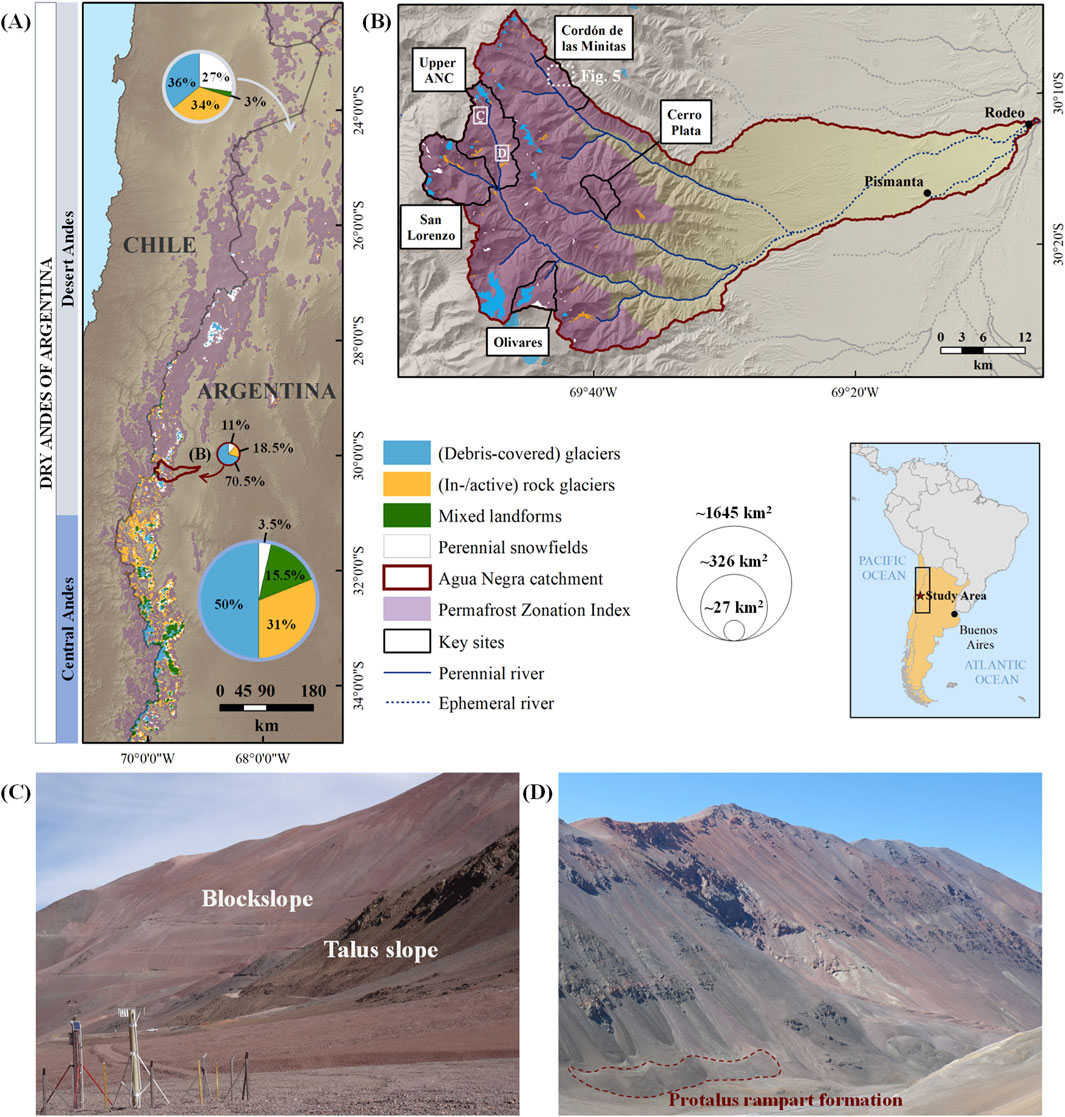
Figure 1. (B) Location of the Agua Negra catchment (ANC) and the key sites used for manual mapping within the cryospheric setting at the transition from the Desert to the Central Andes in the Dry Andes of Argentina (A). Permafrost Zonation Index (very low to high probabilities) based on Gruber (2012) (debris-covered) glaciers, perennial snowfields and (active/inactive) rock glaciers were taken from IANIGLA-CONICET (2018). Pie charts with size encoding are shown to compare the quantity and relative share of cryospheric landforms recorded in the national inventory (IANIGLA-CONICET, 2018) in the Desert Andes (22°-31°S, light grey), the Central Andes (31°-35°S, blue) and the study area (30°S, dark red). (C) View towards SW to predominant block- and talus slopes exposed to NE in the upper catchment area (Photo: Lothar Schrott). (D) View towards SE to talus slopes with protalus rampart formation on the lower talus in the upper catchment area (slope exposition = SW) (Photo: Tamara Köhler).

The Agua Negra catchment (ANC) (∼30°S 69°W) is a high mountain catchment located in the border region between Argentina and Chile in the San Juan province. It lies within the Desert Andes at the southern transition to the Central Andes (see Figures 1A, B). The catchment spans over 1,315 km² and is partially traversed by the transnational pass road Ruta Nacional 150 connecting La Serena (Chile) and San Juan (Argentina).

The ANC covers an altitudinal range of 4,735 m and is drained by the Agua Negra River, which is largely sustained by meltwater from glaciers, seasonal to perennial snowfields, precipitation, and runoff from active layer thawing and permafrost degradation (Halla et al., 2020; Schrott, 1996). Based on Climate Hazards Group InfraRed Precipitation with Station data (CHIRPS), mean annual rainfall between 1981 and 2020 averaged ∼53 mm in the lowland areas of the catchment and increased to 131 mm at higher elevations, suggesting relatively low runoff contributions (Funk et al., 2014). The proportion of rainfall falling as snow versus rain and thus having a delayed or direct effect on runoff remains unquantified. Similarly, infiltration and evaporation losses have not been systematically measured. Still, high regional losses can be inferred from meteorological data collected at a weather station in front of the Agua Negra glacier (30.17°S, 69.80°W, 4,750 m asl), which recorded high global radiation levels of ∼430 W/m² d and low mean relative humidity of ∼30% (Pitte et al., 2022).

Geological data for the ANC is limited to a resolution of 1:250,000 (SEGEMAR, 2019) (see Supplementary Figure S5). The catchment is tectonically active and covers different geological units, including the Agua Negra and San Ignacio Formations composed of Paleozoic marine sedimentary rocks (SEGEMAR, 2019). These are locally intruded by granite causing hydrothermal alterations (Lauro et al., 2017). The Paleozoic basement is overlain by Permo-Triassic and Cenozoic sedimentary, volcanic, and volcanoclastic rocks of the Choiyoi Group and the Doña Ana, Olivares and Cerro de las Tórtolas Formations, with the Choiyoi Group being the predominant unit in the upland area (Heredia et al., 2002; Lauro et al., 2017; SEGEMAR, 2019).

The highest peak reaches 6,280 m asl (sp. Cerro de la Majadita) and hosts the catchment’s largest glacier, covering nearly 10 km². The Agua Negra River originates from the fourth-largest glacier (∼1 km²). The catchment outlet is situated at 1,563 m asl in the small town of Rodeo, located within the intermontane Rodeo-Iglesia Valley between the Cordillera Frontal and the Precordillera (Mardonez et al., 2020). Approximately 50% of the ANC lies above the regional lower permafrost limit at 3,700 m asl (Trombotto, 2000; Gruber, 2012; see Supplementary Figure S4). It features a regionally characteristic, diverse cryospheric landform cover with mainly small (debris-covered) glaciers, seasonal to perennial snowfields, and rock glaciers that visually express the presence of permafrost (see Figure 1B; Table 1). Within the periglacial belt, bare bedrock, block- and talus slopes are predominant (see Figures 1C, D) (Köhler et al., 2024). While no studies confirming Pleistocene glaciations exist for this part of the Andes, scattered morainic remnants and the U-shaped main valley suggest a more extensive past glaciation.

Table 1

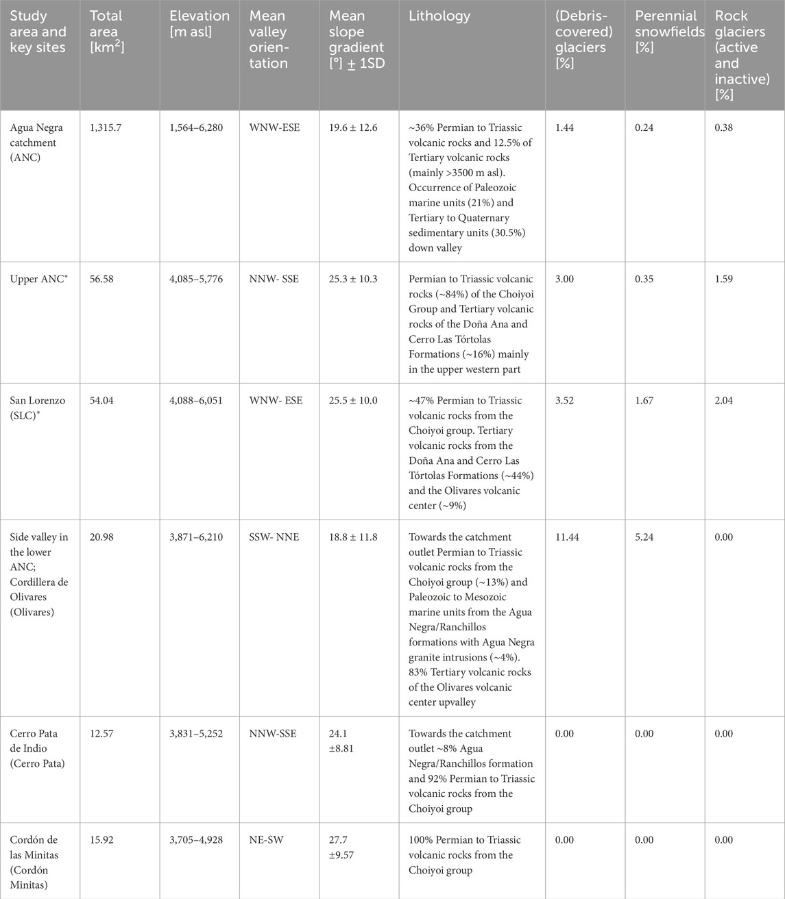
Table 1. Characteristics of the five key sites, the upper Agua Negra catchment (Upper ANC), San Lorenzo catchment (SLC), a side valley further downstream the Agua Negra river (Olivares) and two catchments along its northern tributaries (Cerro Pata, Cordón de las Minitias) (see Figure 1 for locations). (Debris-covered) glaciers, perennial snowfields and (in-)active rock glaciers were taken from the national inventory of cryospheric landforms (IANIGLA-CONICET, 2018). Lithology from SEGEMAR (2019). Mapping results of the marked key sites (*) were revised during a field trip in 02/2022 (field reconnaissance).

Approximately 668 km² of the ANC provide suitable conditions for permafrost, as indicated by the Permafrost Zonation Index (Gruber, 2012). However the national inventory of cryospheric landforms records only 27 km² of mapped features, with rock glaciers as the only periglacial landform recognized (IANIGLA-CONICET, 2018). Over recent decades, their internal structure, kinematics, and ice content have been studied systematically (Blöthe et al., 2020; Brenning, 2005; Halla et al., 2020; Villarroel et al., 2018). This substantial spatial discrepancy inevitably leads to an inaccurate assessment of the periglacial area and its hydrological significance on varying spatial scales.

3 Materials and methods

We applied a raster-based geostatistical upscaling approach using three classification techniques to analyze the distribution and morphometric site characteristics of block- and talus slopes. A combined dataset of manually mapped landforms (dependent response variables) and DEM-derived terrain attributes (independent predictor variables) (see Figure 2; Tables 1, 2) was used to run the different models predicting and explaining the presence and absence of each target landform in the periglacial belt of the ANC.

Figure 2

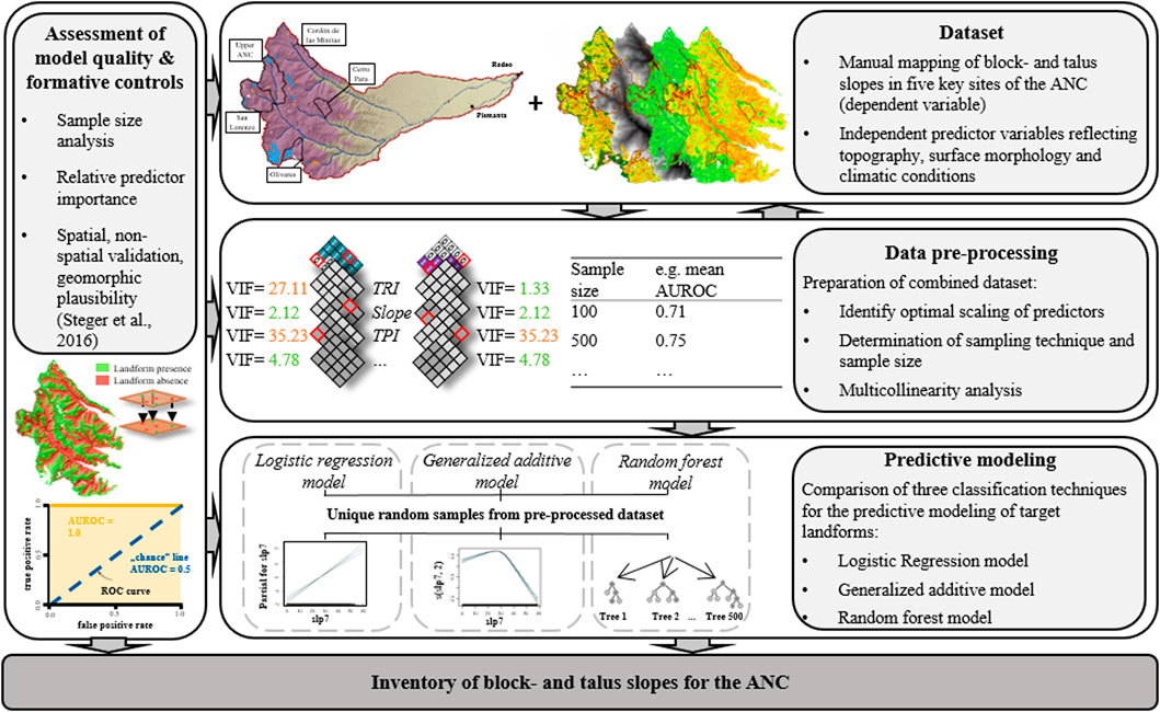
Figure 2. Conceptual workflow for the predictive modeling of block- and talus slopes in the periglacial belt of the Agua Negra catchment (ANC) based on the geomorphological mapping of target landforms in five key sites (for location see Figure 1). (TRI = Topographic Roughness Index, TPI = Topographic Position Index, AUROC = area under the receiver operating characteristics curve).

Table 2

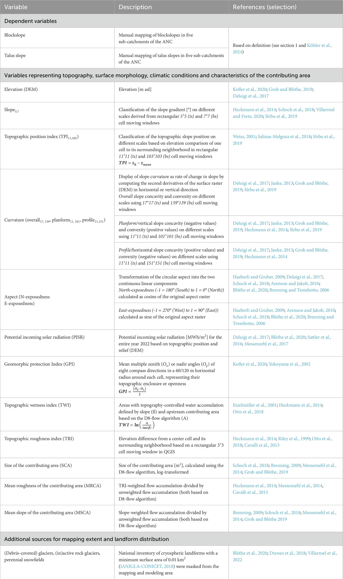
Table 2. Input variables for the predictive modeling of block- (bs) and talus slopes (ts) on different spatial scales (derived from TanDEM-X DEM, resolution: 12 m, DLR 2017). Subscripts indicate optimal moving window sizes for scaling of some predictor variables (Sîrbu et al., 2019). See Supplementary Table S3 for a visualization of the input variables in the modeling domain.

We determined the best trade-off between model performance and interpretability by implementing logistic regression (LR), a generalized additive model (GAM), and random forest (RF). For training and testing, we conducted 10 model runs with 15-fold validation each using stratified random samples from five manually mapped key sites. To contribute to a more accurate assessment of the hydrological significance of cryogenic landforms in the Dry Andes, we focused on areas where ground ice formation is possible within these underestimated periglacial landforms. Thus, the random samples reflected the spatial heterogeneity of block- and talus slope distribution within the periglacial belt of the ANC. The model outputs were validated spatially and non-spatially using statistical measures and geomorphic plausibility (Steger et al., 2016). Additionally, we analyzed the influence of different sample sizes and assessed environmental controls based on predictor importance. The final output consisted of a raster-based distribution map of block- and talus slopes expanding the existing Argentinean national inventory (IANIGLA-CONICET, 2018) and providing information on the distribution and potential permafrost conditions of these landforms.

3.1 Inventory of block- and talus slopes in the Agua Negra catchment

We created a detailed inventory of bedrock, block- and talus slopes (area ≥ 0.001 km²) within five key sites of the ANC using satellite imagery (Esri, Google Earth Pro) and a TanDEM-X DEM with a 12 m resolution (DLR, 2017) (see Table 1, Supplementary Table S3). Satellite images from austral summer months with minimal snow cover and shading were selected to enhance mapping accuracy. All five key sites are located within the periglacial belt (regional lower permafrost limit ≥3,700 m asl, Trombotto, 2000; PZI, Gruber, 2012) (see Figure 1B, see Supplementary Figure S4). The lower limit of 3,700 m is a conservative estimate to encompass the entire regional periglacial belt, though other sources specify limits between 3,900 and 4,000 m asl (Brenning, 2005; Schrott, 1996; Croce and Milana, 2002). The selected key sites span different altitudes, slope angles, valley orientations, and proportions of inventoried cryospheric landform cover to adequately represent the spatial heterogeneity of the ANC (see Table 1; Figure 1). In total, they account for 160 km², corresponding to ∼24% of the study area potentially underlain by permafrost (PZI, Gruber, 2012) and 12.2% of the entire ANC. The key sites serve as (1) example regions to illustrate regional topoclimatic, geomorphologic and cryospheric conditions, and associated processes, (2) manual mapping areas, and (3) calibration and validation areas for the three different modeling techniques.

Mapping results from the first two manually mapped key sites (ANC, SLC) were revised during a field trip in February 2022. Field observations were consistently applied in the subsequent mapping (Olivares, Cerro Pata, Cordón de las Minitas). (Debris-covered) glaciers, rock glaciers and perennial snowfields (area ≥ 0.01 km²) from the Argentinean national inventory of cryospheric landforms (IANIGLA-CONICET, 2018), as well as manually mapped bedrock were masked. The national inventory’s restricted rock glacier delineation excluding frontal and lateral margins (RGIK, 2022), was maintained to ensure model transferability at regional scales. However, we consider the margins of rock glaciers as part of the landform and intentionally left these areas unmapped. A visualization of the mapping results in the three key sites ANC, SLC, and Olivares can be found in Köhler et al. (2024). We mapped only clearly distinct landforms and set the size threshold for consistent and transferable mapping results. Thus, the inventoried landform proportions slightly underrepresent their actual distribution in the ANC. However, the high level of detail of the geomorphological mapping, its validation by three co-authors, and the use of the national inventory (IANIGLA-CONICET, 2018) strongly reduce the uncertainties in the input dataset and thus in the predictive modeling.

3.2 Set of predictor variables for the predictive modeling approach

We used 15 predictor variables derived from the TanDEM-X DEM (void-filled, resolution: 12 m, DLR, 2017) for predictive modeling. The predictors directly or indirectly represented topography, surface morphology, climatic conditions, and contributing area characteristics across different spatial scales (see Table 2, Supplementary Table S3). They characterize the spatial distribution, topoclimatic conditions and geomorphic properties of block- and talus slopes in the ANC (Köhler et al., 2024). For more information, please refer to the companion paper.

By using sine and cosine transformations, circular aspect variables were decomposed into the directional components “north-exposedness” and “east-exposedness” (Brenning and Trombotto, 2006; Brenning, 2009). Climate and moisture conditions are represented by DEM-derivatives due to a lack of measured data in the catchment. Potential incoming solar radiation (PISR) was calculated as the annual sum for 2022. The size of the contributing area (D8-flow algorithm) was log-transformed due to its skewed distribution and wide range of values (Brenning, 2009). The scaling of environmental predictors entering the predictive models is highly dependent on the landform morphometry and its controlling environmental conditions. Thus, we applied an automated scaling procedure (Sîrbu et al., 2019) to identify optimal scaling for slope inclination (slope), topographic position (TPI), and curvature (overall, planform, profile) (see Table 2, Supplementary Table S3). All analyses were conducted in Esri ArcMap (10.4) and open-source GIS and data analysis tools, including QGIS (3.10.9), SAGA GIS (9.3.0), and RStudio (4.3.2).

3.3 Data pre-processing

The quality of the input dataset has a high impact on model quality, robustness and transferability. Various prerequisites were addressed during data preparation: (1) The input data needed to reflect the heterogeneity of the study area (Schoch et al., 2018). (2) the mapped inventory of block- and talus slopes was converted into binary rasters, where “1” indicated landform presence and “0” denoted absence. Each pixel was assigned with the site-specific characteristics of the 15 terrain attributes. (3) (Multi-) collinearity between predictor variables reduces model accuracy and complicates interpretation, as the individual effect of correlated variables on the response variable cannot be determined accurately (James et al., 2013; Heckmann et al., 2014). Thus, geostatistical upscaling requires non-collinearity among predictors, and we computed the variance of inflation factor (VIF) to identify (multi-)collinearity within our predictor set (Aguilera et al., 2006; James et al., 2013). (4) We used different models to predict the probability of a pixel being classified as 1 (blockslope/talus slope presence) or 0 (blockslope/talus slope absence) based on stratified random samples from all key sites. Due to the high blockslope occurrence in the ANC, a ratio of 1:1 (landform presence vs absence) was implemented for each random sample (Brenning, 2005). The aerial share of talus slopes is lower, and thus an even ratio of landform presence and absence in the samples might overestimate the talus slope distribution at the expense of other landforms. Heckmann et al. (2014) note that biases toward small probabilities may occur if the ratio of events to non-events strongly overrepresents one of the cases in the samples. To avoid this and to better reflect the actual conditions, we created random samples with a ratio of 1:3 for talus slopes.

3.4 Predictive modeling of block- and talus slopes

We compared three different classification algorithms to analyze the spatial distribution of target landforms: logistic regression (LR), generalized additive models (GAM), and random forest (RF).

3.4.1 Logistic regression model

LR is one of the most established classification techniques in geomorphology (e.g., Brenning, 2005; Goetz et al., 2015; Marmion et al., 2009; Schoch et al., 2018). LR is a generalized linear model (GLM) commonly used to analyze and predict the probability of a binary outcome (i.e., landform presence or absence) based on a known set of predictor variables using a maximum likelihood approach (Brenning, 2005). GLMs are particularly advantageous when working with spatial data, as they can process different types of statistical distributions and are resistant to model overfitting. In addition, the importance and effect of each predictor on the response variable is comparatively easy to interpret geomorphologically due to the assumed linear relationship (Brenning, 2005; Hjort and Marmion, 2008). The probability of the response variable is calculated as logit or log-odds in the logistic function:

$\mathit{Y}=\mathit{log}\left(\frac{\mathit{p}\left(\mathit{x}\right)}{\mathbf{1}-\mathit{p}\left(\mathit{x}\right)}\right)={\mathit{\beta }}_{\mathbf{0}}+{\mathit{\beta }}_{\mathbf{1}}{\mathit{X}}_{\mathbf{1}}+...+{\mathit{\beta }}_{\mathit{n}}{\mathit{X}}_{\mathit{n}}$

where Y represents the dependent binary response variable with p(x) being the predicted probability of landform presence (Y = 1; blockslope or talus slope present) and 1-p(x) indicating its absence (Y = 0; blockslope or talus slope absent) (Sattler et al., 2016). By computing the log-odds, the odds are transformed into a continuous range that is modeled as a linear combination of n predictor variables (X₁ … X_n) (Heckmann et al., 2014). β₀ is the intercept and β_{1 … n} the coefficients for the set of independent input variables entering the LR, estimated using a maximum likelihood approach (Heckmann et al., 2014; Atkinson et al., 1998). Thus, the model output is the logarithm of odds (log-odds) of the target landforms’ occurrence taking a specific value. It can be converted to predict the occurrence probability of p(x) in a range between 0 and 1 by solving for p(x) (Sattler et al., 2016):

$\mathit{p}\left(\mathit{x}\right)=\frac{\mathbf{1}}{{\mathbf{1}+\mathit{e}}^{-\left({\mathit{\beta }}_{\mathbf{0}}+{\mathit{\beta }}_{\mathbf{1}}{\mathit{X}}_{\mathbf{1}}+\dots +{\mathit{\beta }}_{\mathit{n}}{\mathit{X}}_{\mathit{n}}\right)}}$

For the final prediction of block- and talus slope distribution across the entire ANC, we applied regularized LR for model training and testing. The regularized LR uses all variables from the predictor set but reduces model overfitting and complexity by introducing a penalty term to the loss function that constrains the coefficients, and thus their weight in the model, to be small (Reinwarth et al., 2017). We applied ridge regression, also termed L2 regularization, to retain all variables in the model but penalize them to reduce their magnitude. This method is well-suited when dealing with correlated variables, as it reduces the impact of multicollinearity by constraining the coefficients instead of eliminating them (Reinwarth et al., 2017). Additionally, we implemented an automatic bidimensional stepwise model selection procedure based on the Akaike Information Criterion (AIC) to evaluate predictor variable selection frequency as a measure of their importance (e.g., Heckmann et al., 2014; Schoch et al., 2018; Brenning, 2005).

3.4.2 Generalized additive model

Given the limitations of non-parametric techniques such as GLMs, e.g., inflexibility and lower predictive power (Hjort and Marmion, 2008), we applied further classification techniques. GAMs offer greater flexibility, allowing for linear, complex, and combined relationships between predictor and response variables within the same model while maintaining the interpretability of a LR (Hjort and Marmion, 2008; Hastie and Tibshirani, 1990). As semi-parametric extensions of GLMs, GAMs have been successfully applied in landform distribution modeling (e.g., Brenning and Azócar, 2010; Hjort and Luoto, 2006; Marmion et al., 2009; Schoch et al., 2018). In GAMs, linear and non-linear smooth functions are independently fitted to each predictor variable, with the resulting smoothed curve best representing the effect of the predictor on the response variable (Brenning and Azócar, 2010; Hastie and Tibshirani, 1990). The final model is constructed by summing these smooth functions (Marmion et al., 2009). The flexibility of the smooth functions is determined by the degrees of freedom (df), where higher df allow for more flexible smoothers capable of adapting to more complex data patterns, while at the same time posing a risk of model overfitting (Hastie and Tibshirani, 1990; Wood, 2017). We deployed a stepwise selection of df across 10 model runs with 15-fold validation and identified the best trade-off between over- and underfitting when allowing three df for blockslope and four df for talus slope modeling (see Supplementary Table S1).

In the final model, the response variable is not modeled directly, but as a logit of the probability of landform occurrence as follows:

$\mathit{Y}=\mathit{log}\left(\frac{\mathit{p}\left(\mathit{x}\right)}{\mathbf{1}-\mathit{p}\left(\mathit{x}\right)}\right)={\mathit{\beta }}_{\mathbf{0}}+{\mathit{\beta }}_{\mathbf{1}}{\mathit{f}}_{\mathbf{1}}{\mathit{X}}_{\mathbf{1}}+...+{\mathit{\beta }}_{\mathit{n}}{\mathit{f}}_{\mathit{n}}{\mathit{X}}_{\mathit{n}}$

where Y again represents the dependent binary response variable, β₀ is the intercept, β the coefficients, X represents the individual independent predictor variables, and n is the number of independent predictor variables entering the model. f adds the nonparametric smoothing terms to each predictor, distinguishing GAMs from the LR (Hastie and Tibshirani, 1990). As with LR, we used stepwise variable selection to assess the importance of each predictor based on selection frequency. GAM modeling was performed using the gam and mgcv packages in R (Hastie and Tibshirani, 1990; Hastie, 1992; Wood, 2015).

3.4.3 Random forest model

RF is a non-linear classification technique that is well established in machine learning and increasingly applied in geomorphology (e.g., Blöthe et al., 2020; Brock et al., 2020; Marmion et al., 2009; Goetz et al., 2015; Steger et al., 2016). The dependent response variable is predicted using classification trees based on a set of binary decision rules that determine the class assignment of the response variable according to the predictor variables (Breiman et al., 1984). The model generates a large number of classification trees, each fitted to bootstrapped subsets of the full training dataset with randomly sampled predictors, creating a robust predictor ensemble (“forest”) of decision trees (Brock et al., 2020; Breiman, 2001; James et al., 2013). Class assignment is then predicted through the majority voting across all trees, with the proportion of trees predicting landform presence indicating favorable conditions for landform occurrence and vice versa (Goetz et al., 2015). When building the trees, a newly randomized subset of predictors is chosen as possible split candidates at each split, ensuring that only one predictor from the subset is used per split (James et al., 2013). This condition prevents dominant variables from driving the model and leads to a decorrelation of the variables, thereby mitigating (multi-) collinearity (James et al., 2013; Blöthe et al., 2020). By producing a randomly sampled predictor ensemble of many decision trees, RF effectively captures general patterns in the training data, reducing the risk of variance, overfitting, and sensitivity to noise (Breiman, 2001). Additionally, it is capable of handling complex, non-linear relationships between predictor and response variables (Goetz et al., 2015). At the same time, RF is less interpretable than GAM and LR. However, a summary of the importance of each predictor can be obtained from the model training.

We used 500 classification trees per landform to build up the RF. Predictor importance was determined using a combination of mean Gini-based importance (mean decrease in impurity) and accuracy-based importance (mean decrease in accuracy) (James et al., 2013). We transferred these absolute measures of mean variable importance into relative importance scores across all predictors.

3.5 Assessment of ideal sample size, model quality and formative controls

Sample size can strongly influence model robustness (i.e., reproducibility) and comparability due to over- or underfitting, spatial autocorrelation, and overparameterization (Heckmann et al., 2014). To determine the ideal sample size, we conducted a pixel-based sample size analysis for all three models (number of pixels per sample = 100, 500, 1,000, 2,000, 4,000, 8,000, 16,000, 32,000, 48,000), maintaining predefined ratios of landform presence and absence for both target landforms (1:1 for blockslopes and 1:3 for talus slopes). The optimal sample size was identified based on normalized changes in the area under the receiver operating characteristic curve (AUROC) values and their interquartile ranges (IQR) across ten model runs with 15-fold validation. The ideal sample size was specified by the class above which model improvements became insignificant (defined here as <0.06) or model performance impaired.

We evaluated the predictive power, robustness, and spatial transferability using both spatial and non-spatial validation (Brenning, 2009). Each classification algorithm was trained and tested in 10 model runs with 15-fold validation each, using the ideal sample size determined from the sample size analysis and the predefined landform presence and absence ratios. Unique stratified random samples from all key sites were selected without replacement. We evaluated and compared model performances based on AUROC values, IQR, and model accuracy (sum of the true positive and true negative rate). We transferred probabilities of landform occurrence into binary classes of presence (1) or absence (0) using the optimal cutoff derived from AUROC values, which was further examined for geomorphic plausibility (Heckmann et al., 2014; Steger et al., 2016). The AUROC scores the model performance based on sensitivity (true-positive rate) and specificity (true-negative rate), and ranges from 0.5–1.0 (Brenning and Azócar, 2010). Higher AUROC values signify higher predictive power, with values >0.9 implying an excellent, 0.9 to >0.8 a good, 0.8 to >0.7 a fair, and ≤0.7 a poor model (Araujo et al., 2005). Common non-spatial validation approaches based on splitting one dataset into training and testing subsets have limitations due to dependencies between datasets (Brenning, 2009; Schoch et al., 2018). Therefore, we additionally performed spatial validation (10 model runs, 10-fold validation each) and assessed the geomorphic performance and plausibility in independent test areas outside the training domain (Steger et al., 2016; 2021).

The model whose predictions most closely matched the actual landform distribution (predictive power) and provided consistent results across all model runs both inside (robustness) and outside (spatial transferability) the training domain was identified as the best performing model. This model was then applied to the area above the regional lower permafrost limit (≥3,700 m asl) in the ANC (model domain = 686 km²).

Furthermore, we analyzed the environmental conditions and formative controls of block- and talus slopes based on predictor importance using variable selection frequency (LR & GAM) and relative predictor importance (RF). We evaluated the effect of the influential variables on predicted probabilities to identify key characteristics of block- and talus slopes in the study area.

4 Results

First, we compare the predictive performances of LR, GAM, and RF for both target landforms using non-spatial statistical validation measures. Subsequent analyses, i.e., sample size and spatial transferability, are only presented for the best-performing modeling technique, while more information can be found in the Supplementary Material.

4.1 Comparison of predictive performances and effect of sample size

All models demonstrate good to excellent predictive performances, with mean AUROC values ranging from 0.83 to 0.96 (blockslopes) and 0.85 to 0.95 (talus slopes), along with mean accuracies of approximately 0.82 (blockslopes) and 0.85 (talus slopes) based on non-spatial validation (Araujo et al., 2005) (see Figure 3, Supplementary Table S2). This confirms the model’s ability to distinguish between the presence and absence of the target landforms. Overall, the predictive performance of talus slope modeling is slightly lower and characterized by higher uncertainty compared to blockslope modeling when applying RF and GAM, while the opposite is true for LR.

Figure 3

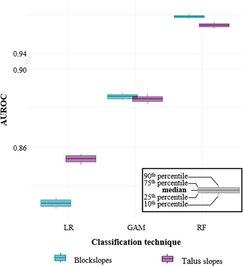
Figure 3. Comparison of the model performances of the three applied classification techniques logistic regression model (LR), generalized additive model (GAM) with three degrees of freedom for blockslopes and four for talus slopes, as well as random forest (RF). Boxplots visualize the area under the receiver operating characteristics curve (AUROC) based on 10 model runs with 15-fold validation. Each model was trained and tested on 32,000 samples with predefined ratios of landform presence and absence (1:1 for blockslopes, 1:3 for talus slopes). See Supplementary Table S2 for exact values.

For both landforms, the predictive ability and geomorphic plausibility of RF clearly outperforms LR and GAM, with LR being least suited in model comparison. The Kruskal–Wallis rank sum test demonstrates statistically significant differences in model performances (p < 0.05) (Schoch et al., 2018). Thus, RF is the most suitable classification algorithm for our predictive modeling approach with small uncertainties, high robustness and good model performance (high AUROC, low IQR).

Increasing sample sizes lead to improvements in AUROC values and reductions in IQR (see Figure 4, for full sample size analysis see Supplementary Figure S1). With the lowest mean AUROC values starting at ∼0.86 and ∼0.82 for block- and talus slopes, respectively, RF performs well even with small sample sizes. However, the smallest sample size class (n = 100) exhibits a comparatively wide IQR (>0.3), indicating lower model robustness and transferability. As sample size increases, AUROC values follow a near-linear progression but show a slight dip at the largest sample size class. For smaller sample sizes (n ≤ 2,000), talus slope modeling yields higher uncertainties and lower predictive power compared to blockslope modeling. However, performance measures converge at sample sizes >2,000. Maximum mean AUROC values of ∼0.96 for both landforms and minimum IQR (≤0.0015) are reached at n = 48,000. The ideal sample size was concordantly established to be 32,000, beyond which model performances hardly improve or possibly even decrease due to overfitting (mean AUROC >0.95, IQR ≤0.0017).

Figure 4

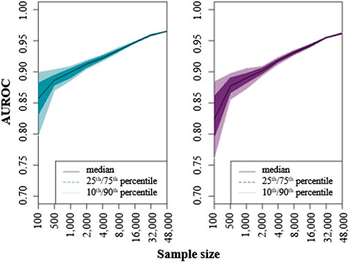
Figure 4. Median, 10th, 25th, 75th and 90th percentile of AUROC (area under the receiver operating characteristics curve) values for different sample sizes derived from ten model runs with 15-fold validation of the random forest model (RF). All random samples from the sample size classes reflect the spatial distribution of block- and talus slopes in the ANC, containing equal pixels of landform presence and absence for blockslopes (ratio 1:1) and a smaller number of pixels with talus slope presence than absence (1:3).

4.1.1 Investigation of geomorphic plausibility and spatial transferability

The key sites selected in this study were chosen to represent the spatial heterogeneity of the ANC (see Figure 1; Table 1) (Köhler et al., 2024). The selection of these diverse key sites is critical for ensuring robust model performance and geomorphic plausibility, which may not be fully captured in purely quantitative validation approaches (Steger et al., 2016; Steger et al., 2021).

Training models exclusively with data from the upper ANC, SLC, and Olivares yields excellent model performance with non-spatial validation (mean AUROC ∼0.96 for both models), but the geomorphic plausibility is poor in distant areas of the ANC (e.g., northern and eastern sections) (see Figure 5A). There, the predictive RF-model mainly confines blockslope occurrences to the uppermost slope positions and low-relief plateaus, while talus slopes are predicted to cover almost the entire vertical extent of the slopes. By incorporating the key sites Cerro Pata and Cordón de las Minitas, we were able to significantly improve model quality in these areas, reduce uncertainty, achieve a clearer model distinction between areas with high and low probability of block- and talus slope occurrence, and thus greatly improve geomorphic plausibility (see Figure 5C).

Figure 5

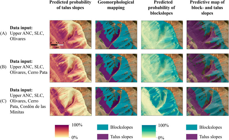
Figure 5. Comparison of the geomorphic plausibility of random forest modeling of block- and talus slopes depending on input data from (A) only the three key sites upper Agua Negra catchment (upper ANC), San Lorenzo catchment (SLC) and the side valley further downstream (Olivares), compared to adding the key site Cerro Pata (B), and using all five key sites for model training (C). Models were trained on 32,000 random samples from the respective key site composition with defined ratios of landform presence and absence (1:1 for blockslopes and 1:3 for talus slopes). See Figure 1 for location of the map section.

Furthermore, we analyzed the importance of individual key sites based on the examination of the spatial transferability with varying test and training key sites. For this, we conducted a spatial validation approach where models were trained on four key sites and tested on a fifth, spatially independent key site (see Figure 6). The results from the spatial validation were compared to the non-spatial validation using the full dataset (“all”, Figure 6).

Figure 6

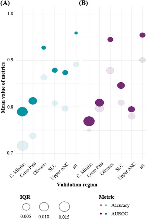
Figure 6. Analysis of the spatial transferability of the random forest model (RF) based on the comparison of predictive performances for (A) blockslope and (B) talus slope distribution in different validation regions (spatial validation). Mean area under the receiver operating characteristics curve (AUROC) and accuracy values (dark and light colored dots) as well as their interquartile ranges (IQR) (dot sizes) are used as performance measures. The predictive performance of the spatial validation is compared with the performance of the non-spatial validation with the full dataset from all five key sites (“all”). Training and testing consisted of ten model runs with 10-fold validation each, using equal sample sizes (=32,000) and landform presence to absence ratios of 1:1 for blockslopes and 1:3 for talus slopes.

Non-spatial validation yields higher predictive performances than spatial validation. However, the spatial validation provides a more realistic assessment of model performance, i.e., when the model was transferred to larger spatial scales (Brenning, 2005; Schoch et al., 2018). Blockslope models exhibit strong predictive power in the upper ANC, SLC, and Olivares but perform less effectively in Cerro Pata and Cordón de las Minitas, aligning with the results from the geomorphic plausibility analysis (see Figure 5). Similarly, talus slope models exhibit lower predictive performance in Cerro Pata, Cordón de las Minitas, and the upper ANC. The IQR are generally higher than for blockslope modeling, signifying greater uncertainty. Thus, a good predictive performance can be assumed when applying the models to the entire ANC (mean AUROC of spatial validation ∼0.85 for blockslopes and ∼0.83 for talus slopes), while the excellent model performance revealed by non-spatial validation is likely limited to the key sites or areas with similar environmental conditions.

4.1.2 Importance of predictor variables

The predictor variables included in the RF model vary in terms of their relative importance (see Figure 7). Predictors classified as independent through multicollinearity analysis can be analyzed without restriction, whereas weakly collinear variables require cautious interpretation. We identified a slightly critical multicollinearity (VIF 10 to ≤13.5) for sr, twi, SCA, MSCA and MRCA in blockslope modeling and for sr, MSCA and MRCA in talus slope modeling. A VIF exceeding 10 indicates problematic collinearity (Heckmann et al., 2014). All remaining variables remained below this threshold and are thus considered as independent.

Figure 7

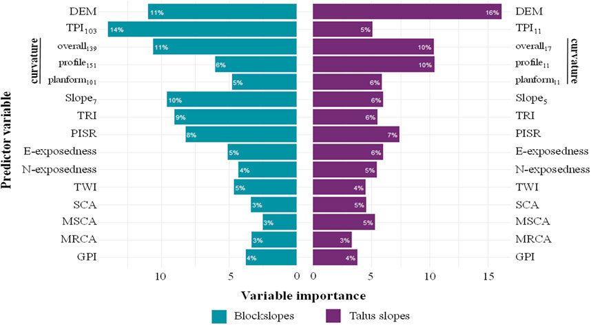
Figure 7. Comparison of relative predictor variable importance for block- and talus slope distribution based on ten model runs of random forest (RF) with 15-fold validation each (sample size 32,000 with a 1:1 ratio of blockslope and 1:3 talus slopes presence vs absence). The variable importance is derived as relative importance compared to the total importance across all predictors.

In descending order of importance with relative shares of ≥10%, the most influential predictors for blockslope modeling are topographic position (TPI₁₀₃), altitude (DEM), overall terrain curvature (curv₁₃₉) and slope inclination (slope₇). Although both variables are deemed less critical for blockslope prevalence, profile curvature₁₅₁ (6%) plays a more significant role than planform curvature₁₀₁ (5%). Furthermore, topographic roughness (TRI, 9%) and potential incoming solar radiation (PISR, 8%) are important predictors for blockslope distribution, whereas contributing area characteristics (MRCA, MSCA, SCA) tend to play a minor role (3%). Regarding aspect, the importance of E-exposedness slightly outweighs that of N-exposedness.

The variable importance ratio is more balanced in the talus slope model. Altitude is by far the most influential predictor (16%) for talus slope distribution in the study area, followed by overall curvature₁₇ and profile curvature₁₁, each contributing 10%. PISR, E-exposedness, slope₅, planform curvature₁₁ and TRI are of intermediate importance (6%–7%). Similar to blockslopes, E-exposedness slightly outweighs N-exposedness. However, characteristics of the contributing area, particularly the mean slope inclination (MSCA) and mean roughness (MRCA), are more decisive for the distribution of talus slopes than for blockslopes, whereas topographical position (TPI₁₁) is less important. The least influential predictor (3%) is the size of the contributing area (SCA).

Thus, the models exhibit few similarities. Except for sr in both landform models, variables with slight collinearity tend to play a minor role. The influence of multicollinearity is further reduced by employing random forest for our predictive modeling approach. This allows us to analyze the relationships between the most important predictors and the distribution of target landforms in more detail. The variable importance analysis based on selection frequency using LR and GAM is presented in the Supplementary Material (see Supplementary Figure S2).

4.2 Block- and talus slope distribution in the Agua Negra catchment

Modeled block- and talus slope coverage revealed that both landforms account for almost 79% of the area above the regional lower permafrost limit (3,700 m asl) and exhibit a distribution ratio of ∼61% (blockslopes) to ∼17% (talus slopes), similar to the key sites (see Figure 8A; Table 3). Overlapping predictions affect approximately 5% of the modeled block- and talus slope area, primarily in the eastern, lower part of the ANC towards the lower permafrost limit and thus the model boundary (see Figure 8B). Elsewhere, the overlaps are minimal and mainly confined to transitional zones between block- and talus slopes in middle slope positions and areas with small to medium-sized bedrock outcrops. The remaining 21% of the model domain, not covered by either the target landforms or the inventoried cryospheric landforms (IANIGLA-CONICET, 2018), is occupied by other landforms, including bedrock, alluvial fans, and floodplains, which are beyond the scope of this study. These features are correctly excluded from both models, while frontal and lateral aprons of rock glaciers, which are not included in the national inventory (restricted rock glacier delineation, see Section 3.1) are typically interpreted as talus slopes. The model slightly underestimates the distribution of blockslopes compared to manual mapping, whereas no clear: trend is observed for talus slopes (see Table 3). Only in Cordón de las Minitas, both models overestimate the respective landform distributions, while the largest deviation occurs at the Olivares key site. On average, the predictive models exhibit a negative offset of −3% for blockslopes and a slightly positive offset of 0.5% for talus slopes. However, the overlap has to be considered when interpreting these values.

Figure 8

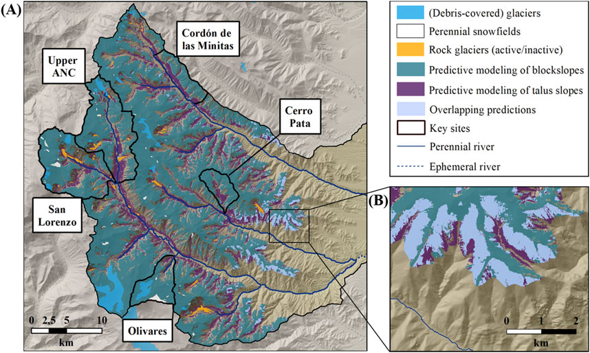
Figure 8. (A)Modeled block- and talus slope distribution above the regional lower permafrost limit (≥3,700 m asl, 686 km²) in the ANC based on random forest modeling (RF). Model outputs were classified based on the statistically derived optimal cutoff values and slightly corrected for talus slopes after examining their geomorphic plausibility in the entire ANC. Part of the overlap in the western lower ANC is shown enlarged (B). (Debris-covered) glaciers, perennial snowfields and rock glaciers from IANIGLA-CONICET (2018).

Table 3

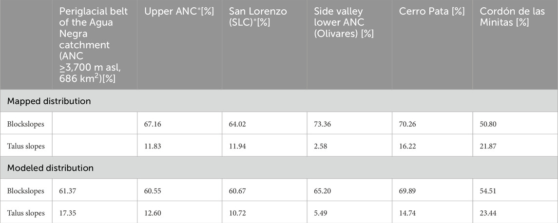
Table 3. Presentation of the mapped and modeled distribution of block- and talus slopes in the key sites and the periglacial belt of the ANC. Manual mapping in the marked key sites (*) was verified during fieldwork in 02/2022. Modeling was performed using a random forest model trained on 10 model runs with 15-fold validation each. 32,000 random samples with defined landform presence and absence ratio (1:1 for blockslopes and 1:3 for talus slopes) were taken for training and testing.

The relationship between the most influential predictor variables in the RF model (see Section 4.1.2) and the predicted probability of block- and talus slope occurrence highlights heterogeneous distribution conditions for both landforms. General trends rather than specific statements can be drawn from this. Most predictors show non-linear relationships with both landforms (see Figure 9, for all variables see Supplementary Figure S3).

Figure 9

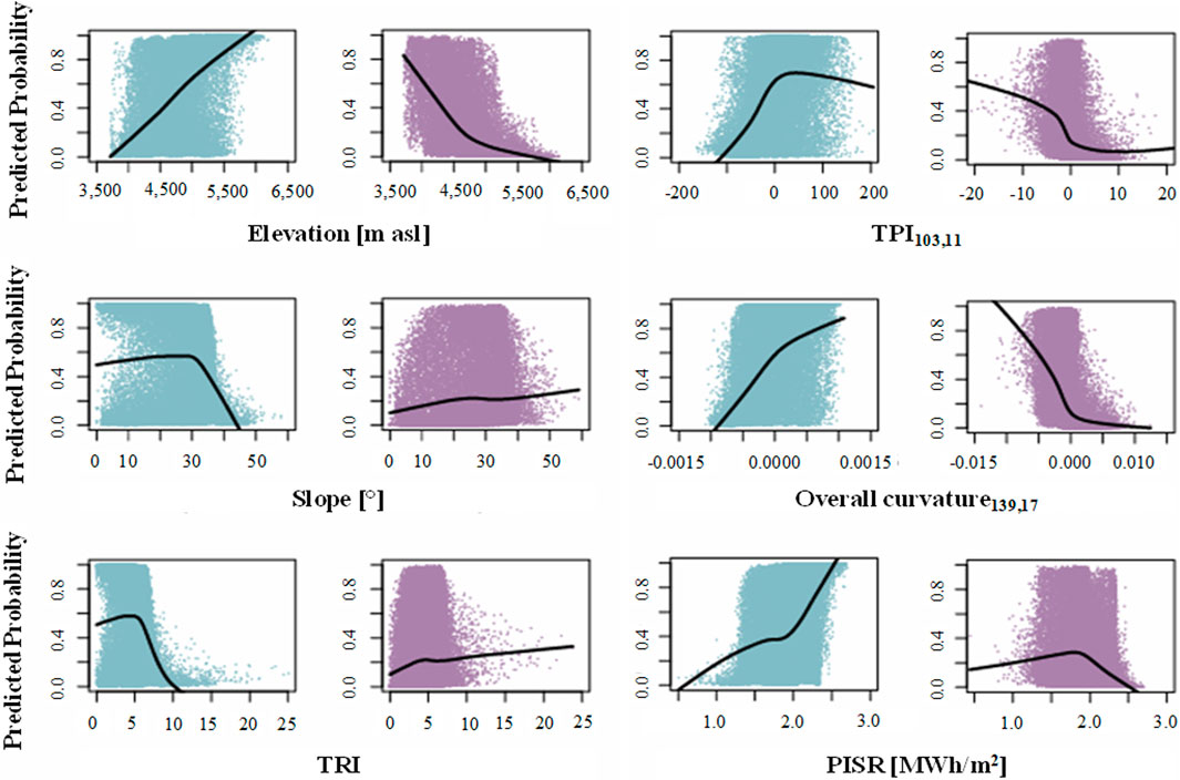
Figure 9. Comparison of the effect of influential predictor variables on the predicted probabilities of block- (light blue) and talus slopes (light purple) in the periglacial belt of the ANC. TPI = topographic position index, TRI = topographic roughness index, and PISR = potential incoming solar radiation for the entire year 2022. Note the different x-axis scaling for TPI_103,11 and overall curvature_139,17 for block- and talus slopes. See Supplementary Figure S3 for comparison of all applied predictor variables.

Blockslopes occur at all modeled elevations and at various topographic positions but become more probable with higher elevations and slope positions. Peak probabilities around 0.8 at neutral to moderately positive TPI₁₀₃ values confirm this and indicate their primary occurrence on middle to upper, open slopes with constant inclination or low-relief areas. Blockslopes show a bimodal distribution at lower slope angles (≤15°), displaying either very high or very low predicted probabilities. The maximum likelihood of blockslope presence is observed at 30°–35°. Above this value, the probability declines, making their classification highly unlikely at slopes >45°. Blockslopes have minimal dispersion around zero for the overall curvature (curv₁₃₉ ± 0.0015), suggesting they are vertically and horizontally elongated with minor lateral convexity and upward concavity. Their highest predicted probabilities are associated with low roughness values (TRI) < 10. Potential incoming solar radiation (PISR) has a considerable effect on the prediction of blockslopes. Blockslopes are rare and highly unlikely below a PISR of ∼1.3 MWh/m² but become significantly more frequent above this value. However, occurrence probabilities exhibit high dispersion. Blockslope probability only begins to decline at approximately 2.4 MWh/m². In contrast to talus slopes, however, they continue to occur frequently and exclusively with high likelihoods.

Talus slopes are predominantly located at foot slopes towards the valley bottom or at cliff bases, with the highest predicted probabilities at low TPI₁₁ values. TPI₁₁ ∼0 indicate their occurrence on open slopes with constant inclination or flat areas (Weiss, 2001). These locations are primarily in proximity to major bedrock outcrops, below large headwalls and within the rooting zones of inventoried rock glaciers (IANIGLA-CONICET, 2018) (see Figures 8, 9). Supporting this, talus slopes reach highest probabilities between 3,700 m asl (lower limit of predictive modeling approach) and ∼4,000 m asl. With increasing altitude, they become less likely, rarely existing above 5,000 m. Talus slopes display low sensitivity to slope angle, primarily occurring between 20°–40° in the study area. Overall curvature ∼0 confirms that talus slopes are vertically and horizontally planar, thus slope angles vary only slightly. They are mostly distributed at TRI values <10, with a few occurrences at higher values. There, they are more likely to occur than blockslopes. In general, talus slopes are less sensitive to the amount of incoming solar radiation and occur across all recorded PISR quantities. Yet, the parameter is ranked with high importance by the RF model, and a negative correlation is observed beyond a potential annual budget of ∼1.8 MWh/m². With increasing PISR, the likelihood of talus slope formation declines to almost 0% above ∼2.3 MWh/m².

5 Discussion

5.1 Model prerequisites for predicting block- and talus slope distribution and their limitations

The consistently high predictive performances of the RF model with low uncertainties suggest that RF effectively captures the distributional characteristics of block- and talus slopes in the ANC. The significantly poorer performance of LR compared to GAM and RF (see Figure 3) demonstrates that the widespread, heterogeneous distribution of talus slopes, and even more so of blockslopes, requires modeling techniques that can cope with these heterogeneous, often non-linear relationships. The superior model performance of RF in the sample size analysis (see Supplementary Figure S1) highlights the advantages of data-driven over more model-driven classification algorithms when working with complex, non-linear data, although a thorough examination of model plausibility is required (Breiman, 2001; Schoch et al., 2018; Steger et al., 2021). However, achieving good to excellent model performance requires careful consideration of various prerequisites and limitations:

1. Addressing mapping uncertainties: Geomorphological mapping based on remotely sensed imagery is subject to uncertainties. These should be minimized to ensure high accuracy in predictive modeling. Some studies demonstrate large mapping heterogeneities of up to 30% due to variable image resolution and quality, inter-operator mapping style, and a lack of established guidelines for landform classification and mapping, with the latter two appearing to produce the highest uncertainties (Brardinoni et al., 2019; Paul et al., 2013). It is recommended to provide transparency on how the mapping was compiled to support accuracy assessment and, if possible, to obtain reference data (e.g., higher resolution satellite data) to better quantify mapping inaccuracies (Chandler et al., 2018; Smith et al., 2006). In data scarce regions like the Dry Andes of Argentina, reference data is often not available. Thus, transparency about the datasets and software used, the mapping procedure, landform definitions, and associated errors and uncertainties is imperative. To minimize inaccuracies in our inventory, we (1) used satellite imagery from austral summer with minimal snow and cloud cover. (2) Prior to mapping, we established consistent definitions and respective guidelines for mapping block- and talus slopes (see Section 1), and (3) the results of the first two manually mapped key sites were revised in the field (ground truthing). (4) Mapping was performed by one operator and reviewed by three co-authors before entering the predictive models. (5) The combination with the national inventory (IANIGLA-CONICET, 2018) prevents an overestimation of block- and talus slopes at the expense of these cryospheric landforms. Still, mapping uncertainties exist due to the medium resolution of the available data (Google Earth Pro, TanDEM-X DEM and derivatives at 12 m resolution) and the associated size threshold for landforms. Working in areas with limited data availability is intertwined with higher uncertainties, but yields valuable and needed information.

2. Predictor selection and processing per landform: To construct and compare reliable predictive models, the choice of predictors should be carefully examined and, if necessary, adapted during the modeling process (Heckmann et al., 2014). RF successfully excludes areas with favorable conditions for the alternative target landform in most of the ANC, indicating a strong alignment between the selected variables and the underlying geomorphological processes. To minimize overlap at the margins of the model domain, incorporating relative position indices, such as distance to ridge, alongside absolute position information (DEM, TPI_11,103) could improve accuracy. Additionally, expanding mapping and modeling beyond the area of interest may further reduce model boundary effects. The model’s performance depends on the quality of the input dataset, which must adequately represent all relevant geomorphologic processes and conditions. According to Brenning (2005), cofounding parameters such as east-exposedness and elevation may provide indications of geological units in large-scale modeling along the north-south-trending Andes. Still, we acknowledge the influence of lithology on the geomorphological processes and the resulting debris properties acting on block- and talus slopes that we cannot adequately account for.Implementing an optimal scaling analysis for certain predictor variables significantly enhanced the predictive performance for both landforms and should be applied to identify and further refine the distinction between both landforms. In addition, we recommend using models that can adequately capture the non-linear relationships in block- and talus slope modeling.

3. Number of random samples: Robust distribution predictions across the entire ANC require a high number of samples with representative cases and controls of the target landforms. The large sample size required indicates that block- and talus slopes occur in a heterogeneous environment, necessitating large training datasets to distinguish between favorable and unfavorable site conditions. Whilst smaller sample sizes can still yield reasonably accurate predictions, the uncertainties in the (non-)spatial validation can be much improved by increasing the number of samples. However, the effect of large sample sizes should be analyzed carefully to prevent overfitting, overparameterization, and spatial autocorrelation, which can result in models with low robustness, poor transferability, and reduced predictive performance (Heckmann et al., 2014; Hjort and Marmion, 2008).

4. Reflection of spatial heterogeneity: Representative, spatially separated training and testing datasets ensure that the model’s predictive performance remains robust, transferable, and geomorphically plausible at larger spatial scales (Schoch et al., 2018; Steger et al., 2016). Block- and talus slopes occur under highly variable environmental conditions in the Dry Andes that need proper reflection in the training data. Including information from multiple key sites with distinct environmental characteristics is necessary to achieve excellent model performances across the entire model domain. Hence, the use of sufficiently large, representative and spatially independent samples from comparable key sites is needed to provide a proper base for a reliable geostatistical upscaling of block- and talus slopes.

5. Safeguarding model quality: Our results illustrate the importance of spatial validation and geomorphic plausibility analysis next to the more commonly used non-spatial validation (see Figures 5, 6) (Schoch et al., 2018; Goetz et al., 2015; Brenning, 2009; Steger et al., 2016). Since these more accurately reflect the model’s actual performance, especially when applied to larger spatial scales (e.g., the ANC), they should be consulted in statistical evaluations of each model. By repeatedly training and testing the model using spatial and non-spatial validation, as well as geomorphic plausibility, we can present two robust and transferable models with good predictive performances for block- and talus slopes in the ANC. In addition, ground truthing via field work is time-consuming but crucial when relying primarily on satellite data to ensure that the model is trained on accurate and consistent input data, adequately representing general and distinctive features of the study area (Brenning, 2005).

5.2 The geomorphological niche of block- and talus slopes in the Dry Andes of Argentina

We identified several topoclimatic and geomorphic conditions that favor or inhibit the formation of block- and talus slopes. Conversely, their occurrence provides important insights into their surrounding environment (Brenning, 2005; Messenzehl et al., 2017).

Blockslopes are dominant mesoscale landforms in the periglacial belt and are found primarily at altitudes above 4,000 m in the ANC. They occupy open middle to upper slopes, gently sloping lateral and horizontal ridges, and low-relief plateaus. Slope angles are evenly distributed up to 35°, but remain largely constant along individual slopes. Garleff and Stingl (1983) found an almost uniform distribution of all slope inclinations up to ∼35° on blockslopes in the semi-arid Andes, similar to findings by Clow et al. (2003) in the Colorado Front Range. However, they generally exhibit a narrower range of slope angles around 20°–38°, depending on the angle of repose of the prevailing bedrock (e.g., Selby, 1974; Ballantyne, 2018; French, 2017; Fort and van Vliet-Lanoe, 2007). Unlike talus slopes, blockslopes are covered by finer surface material, with no indications of grain-size induced sorting, and are intersected by small, isolated and resistant bedrock outcrops. They are often bounded downslope by large rock formations, talus slopes, and rock glaciers. Where these landforms do not limit blockslope propagation, they occupy entire slopes down to the valley bottoms. Extensive blockslope coverage down to the basal slope is mostly found on NE-exposed slopes of the ANC, while SW-exposures are dominated by an upslope sequence of talus slopes, bedrock, and blockslopes with occasional bedrock outcrops (see Figure 8). Blockslopes demonstrate a distinct horizontally and vertically elongated, undissected morphometry that has also been described in numerous studies (e.g., French, 2017; Köhler et al., 2024; Garleff and Stingl, 1983; Höllermann, 1983), contributing to their varying terminologies (compare Section 1). Processes such as erosion, accumulation, channeling, and gully formation are mostly absent, as confirmed by field observations and geomorphological mapping. Local incision is limited to snow and glacier meltwater streams, and major erosion and deposition are more likely to be anthropogenically induced (e.g., road construction, see Figure 1C). Their topographic position, shape and characteristics of the contributing area do not promote the production and deposition of allochthonous material (Weiss, 2001). Unlike talus slopes, they are least likely to develop beneath extensive bedrock outcrops with ongoing rockfall activity and steep, laterally converging topography. Blockslopes are described as characteristic features in upland areas with relatively uniform geology and high porosity that have not been affected by glacial steepening (Ballantyne, 2018; Trombotto Liaudat et al., 2014; Selby, 1974). Although the resolution of the available geological data does not allow for more precise statements, this observation aligns with the widespread occurrence of blockslopes in the relatively homogeneous geology of the ANC (see Table 1, Supplementary Figure S5). These observations support their classification as allochthonous debris deposits (Ballantyne, 2018; Höllermann, 1983; van Steijn, 2002; Otto, 2006; French, 2017; Trombotto Liaudat et al., 2014).

The altitude, position-dependent distribution, and topographic openness of blockslopes suggest climatic control factors, e.g., exposure to high solar radiation, large seasonal and diurnal temperature fluctuations, and wind action. Due to its subtropical location, the ANC experiences exceptionally high solar radiation, comparatively low cloud cover throughout the year, and low solar absorption by atmospheric constituents (Schrott, 1998; Viale et al., 2019; Barry and Chorley, 1992). Peaks in global radiation exceeding 1400 W/m² and maximum daily sums of 35.6 MJ/m² were recorded above 4,000 m asl by Schrott (1998) in December 1990 and 1991, which is roughly consistent with more recent measurements by Pitte et al. (2022) (see Section 2). Although aspect and PISR are not the primary drivers of block- and talus slope distribution, their influence is evident in the observed asymmetric zonation, with more extensive blockslope distribution on NE-facing slopes (see Figure 8). The high prevalence of blockslopes on exposed upper slopes, gently inclined ridges, and low-relief plateaus favors high solar irradiation, aridity, and elevated ground temperatures depending on altitude, which also influences the formation of permafrost (Gruber, 2005; Arenson and Jakob, 2010). Decreasing landform probabilities with rising topographic wetness indices (TWI) further indicate that blockslopes form in well-drained, arid areas, although both target landforms are generally associated with dry conditions (low TWI), consistent with the dry climatic conditions in the ANC (see Section 2) (Pitte et al., 2022; Schrott, 1998). In addition, the high exposure of blockslopes to wind action results in minimal snow cover and duration, further promoting dryness and little protection against temperature fluctuations throughout the year (Clow et al., 2003; Köhler et al., 2024). This leads to intense physical weathering under extremely cold and arid conditions, which is strongly associated with blockslope formation (e.g., French, 2017; Fort and van Vliet-Lanoe, 2007; Iwata, 1987; Trombotto Liaudat et al., 2014). Intensive physical rock decomposition, mainly caused by salt weathering and frost action, is considered to be the dominant driver in forming the thin debris layer covering the retreating bedrock they develop on (Trombotto Liaudat et al., 2014; Ballantyne, 2018; Shaw and Healy, 1977; Höllermann, 1983). Brettschneider (1980) recorded the highest weathering intensities on subtropical sun-exposed mountain slopes around 30°, aligning with the maximum blockslope distribution between 30° and 40°S on the Southern Hemisphere (Höllermann, 1983).

Grain size compositions range from mainly silt to medium and coarse sand, with surface clasts primarily consisting of block-sized debris (Otto, 2006; Selby, 1974; Garleff and Stingl, 1983). The thin debris layer varies from decimeters to several meters in thickness (Ballantyne, 2018; Fort and van Vliet-Lanoe, 2007; Garleff and Stingl, 1983). Downslope movement occurs at low velocities through various processes, including solifluction, frost creep, and potentially permafrost creep, depending on the presence of ground ice (Ballantyne, 2018; Selby, 1974; Fort and van Vliet-Lanoe, 2007; Garleff and Stingl, 1983). Denudation by wind action, rather than linear erosion, is responsible for debris removal along slopes (French, 2017; Selby, 1974; Otto, 2006; Höllermann, 1983). Limited downslope accumulation produces a slight basal concavity (slightly positive profile curvature₁₅₁, see Supplementary Figure S3), and may also be a relic of the ANC’s glacial legacy. Still, material supply and removal appear to be in a dynamic equilibrium, resulting in the characteristic rectilinear shape of blockslopes (e.g., Trombotto Liaudat et al., 2014; Ballantyne, 2018; French, 2017; Brenning, 2005). With increasing elevation, unvegetated, rocky blockslopes become predominant in the ANC. However, in climatically suitable areas at lower altitudes, a sparse vegetation composed of adapted species was observed in the field, suggesting an overall lower level of process activity.

Even sparse vegetation cover is almost absent on active talus slopes, indicating much higher process activity on one of the most common debris storage landforms in mountain environments (Messenzehl et al., 2017; Sass, 2006; Phillips et al., 2009; Scapozza et al., 2011). In the Dry Andes above 3,700 m asl, talus slopes extend up to 5,000 m asl, favoring large contributing areas (≥10³ m²) with steep, massive bedrock outcrops. Therefore, they are mostly concentrated on middle to lower slopes below ascending headwalls, cirques, rock glacier rooting zones, or cliff bases. They may extend into the floodplain, where they are partly covered by alluvial fans and eroded by fluvial processes (Alonso and Trombotto Liaudat, 2013; Köhler et al., 2024). Their vast distribution is embedded in a heterogeneous, rugged terrain with juxtaposed small-to large-scale landforms (Messenzehl et al., 2017). Talus slopes are more prevalent on SW-facing lower slopes in the ANC, resulting in lower exposure to solar radiation (see Figures 8, 9). As PISR is ranked with medium to high importance by the RF, talus slope formation is favored by topographically induced shading, leading to cooler conditions year-round (Phillips et al., 2009).

Köhler et al. (2024) identified the characteristics of the contributing area as useful indicators for analyzing and distinguishing the distribution of target landforms, as they relate to the type of material supply (in situ or ex situ), process intensity, and topographic position. This is confirmed by the greater influence of these variables on the prediction of talus slopes, consistent with their formation by gravitational processes from adjacent steep slopes (Brenning, 2005; Moore et al., 2009; Ballantyne, 2018; Alonso and Trombotto Liaudat, 2013). While the probability of blockslopes decreases with increasing mean slope and roughness of the contributing area (MRCA, MSCA), talus slopes become more likely (see Supplementary Figure S3). Since rockfall activity and granular disintegration of cliff faces are the primary sources of talus accumulation, their formation is mainly controlled by weathering and topography, forming steep and thick talus deposits of varying sizes and shapes over time (Brenning, 2005; Ballantyne, 2018; Messenzehl et al., 2017; Clow et al., 2003). Their slope inclination corresponds to the angle of repose of the coarse rockfall material, resulting in a much higher prevalence of talus slopes with angles >35° than blockslopes. Slope gradients between 31° and >40° are frequently reported (Clow et al., 2003; Messenzehl et al., 2017; Scapozza et al., 2011).

The ANC encompasses a wide range of talus slopes that vary in size, shape and thickness depending on the characteristics of the adjacent bedrock, and topography. Talus material may be redistributed by snow avalanches, fluvial processes, and debris- and dry grain flows (Otto, 2006; van Steijn, 2002). Compared to blockslopes, these landforms are significantly smaller and more spatially confined, as reflected in the smaller optimal moving window sizes determined for predictive modeling (Sîrbu et al., 2019). We identified the three main types of talus slopes through geomorphological mapping and field observations: (1) talus sheets with fairly uniform rockfall activity, along with widespread (2) talus cones, and (3) coalescing talus cones, formed by extensive channeling of rockfall debris and lateral merging of individual cones (see Figure 1D) (Ballantyne, 2018; Brenning, 2005). The accumulation and channelization of material favor the formation of talus sheets and cones in the ANC, supported by the greater influence of horizontal (profile) and vertical (planform) curvature in the predictive modeling of talus slopes than in blockslopes. In addition to their predominantly straight shape, talus slopes exhibit a slight tendency toward upward convexity and lateral concavity, indicating horizontal material deposition and vertical convergence of flow (see Figure 9 and Supplementary Figure S3) (Etzelmüller et al., 2001; Sîrbu et al., 2019; Deluigi et al., 2017). Although talus slopes also have low topographic wetness indices, the conditions for moisture concentration are more favorable. Their environmental characteristics promote higher water availability and moisture storage capacity due to reduced exposure to wind and sun. Local snow accumulations are often found at upper talus slopes, especially below large rock cliffs (Brenning, 2005). During field work, we frequently observed erosion rills, debris flows, and alluvial channels likely attributed to meltwater on the surfaces of talus slopes, which could not be captured in the models due to the coarse resolution (Brenning, 2005). The cold climate of the ANC promotes strong physical weathering with frost action and frequent freeze-thaw cycles resulting in bedrock fracturing, and rockfall activity, thus acting as a sediment source (Clow et al., 2003; Messenzehl et al., 2017; Matsuoka and Murton, 2008).

Field observations confirmed a much coarser, poorly sorted debris composition than on blockslopes. Subsurface investigations reveal layers of coarse, open-work material with a higher proportion of decimeter-to meter-sized boulders at the surface and basal talus overlying interbedded fine and coarse-grained clastic material (Ballantyne, 2018; Sass, 2006; Clow et al., 2003; Lambiel and Pieracci, 2008; Scapozza et al., 2011). The deposition of finer material mainly covering silt, sand, and gravel implies that talus formation is not only driven by rock fall deposition but also by alluvial deposition from disintegrated material from source rockwalls (Ballantyne, 2018; Clow et al., 2003). Studies from the Alps and Svalbard using geophysical methods found sediment thicknesses of 3–45 m overlying bedrock (e.g., Hoffmann and Schrott, 2003; Sass, 2006; Clow et al., 2003; Lambiel and Pieracci, 2008). In periglacial environments, talus deposits often contain varying amounts of ground ice and their formation is frequently modified by processes such as periglacial creep, snow avalanches, and debris flows (Ballantyne, 2018; Scapozza et al., 2011; 2015; Sass, 2006; Hilbich et al., 2022). In such environments with ongoing creep, talus slopes may evolve into protalus ramparts and rock glaciers (Otto, 2006; Ballantyne, 2018; Buckel et al., 2021; Scapozza et al., 2011). Their dominant formation at the foot of rockwalls on glacially oversteepened valley sides and cirques in the ANC is conditioned by the glacial heritage that enhances talus supply (Brenning, 2005; Messenzehl et al., 2017). Despite missing information on past or present glacier retreat, increased paraglacial rockfall activity on talus slopes following glacier recession is expected in the ANC (Brenning, 2005).

5.3 Toward a more comprehensive cryospheric landform inventory of the ANC?

Using geomorphological mapping and predictive modeling, we significantly reduced the spatial discrepancy between the cryospheric landforms recorded in the national inventory (∼27 km²) and the area potentially underlain by permafrost (regional lower permafrost limit ≥3,700 m asl, ∼686 km² (Trombotto, 2000; Esper Angillieri, 2009); PZI ∼668 km² (Gruber, 2012)). Approximately 516 km² (>75%) of the area is covered by block- and talus slopes, making them extremely abundant in this part of the Dry Andes.

Rock glaciers are the most prominent permafrost landforms in the periglacial belt of the Dry Andes, and their formation and topoclimatic conditions result in a higher permafrost content and thus greater hydrological significance than other periglacial landforms (Corte, 1978; Halla et al., 2020; Arenson and Jakob, 2010; Jones et al., 2019; Schaffer et al., 2019). Beyond these, however, knowledge about permafrost distribution and fresh water storages in periglacial landforms remain limited, despite growing evidence of ground ice presence in areas without rock glaciers (e.g., Hilbich et al., 2022; Mathys et al., 2022; García et al., 2017; Arenson and Jakob, 2010). For the Dry Andes of Argentina, the PZI (Gruber, 2012; see Figure 1, Supplementary Figure S4) and the regional permafrost distribution model developed by Tapia Baldis and Trombotto Liaudat (2020) show that permafrost is not restricted to rock glaciers. Low MAAT at high altitudes, strong temperature gradients, and the rugged mountain topography with varying exposures promote frost action, mechanical weathering, and associated geomorphological processes that define the periglacial domain (French, 2017; Trombotto, 2000). Garleff and Stingl (1983) describe the intensive weathering with high fine material production as a characteristic feature of the semi-arid periglacial stage that is further enhanced by pronounced temperature fluctuations and frequent frost cycles. In addition, widespread and intense rockfall activity produces large accumulations of coarse debris (Lauro et al., 2017; Halla et al., 2020). Depending on the thickness and physical properties of the debris layer, these accumulations effectively insulate the ground and thus provide favorable conditions for ground ice formation and preservation (Arenson et al., 2022). High insolation and wind action, low cloud cover, relative humidity, and precipitation contribute to high sublimation rates and a thin, short-lived seasonal snow cover (Pitte et al., 2022; Ayala et al., 2023; IANIGLA-CONICET, 2018; Brenning, 2005). Minimal snow cover offers fragmented protection against rising summer temperatures and radiation exposure, especially on exposed blockslopes (Arenson et al., 2022; Delaloye et al., 2003; Selby, 1974; Morard et al., 2010). Simultaneously, these conditions reduce the diurnal to seasonal effect of snow insulation and allow deep penetration and circulation of cold air, depending on the physical properties of the debris layer, in winter (Phillips et al., 2009; Lambiel and Pieracci, 2008; Morard et al., 2010). This distinctive thermal regime favors permafrost conditions and ground ice formation, underscoring the high potential of yet unidentified freshwater resources in the periglacial belt of the Dry Andes. Based on our findings, we can evaluate the conditions for the formation and preservation of permafrost based on the environmental distribution conditions of block- and talus slopes.

Overall, the probability and extent of permafrost are significantly higher in talus slopes than in blockslopes due to their differences in spatial distribution and formation conditions. The topoclimatic and geomorphologic characteristics of talus slopes result in thick, coarse debris deposits, greater topographic shading, snow accumulation, and enhanced moisture availability, creating much more favorable conditions for permafrost occurrence. The coarse, open-work debris accumulations lead to high air content near the surface, facilitating deep penetration and circulation of cold air within the talus deposits (Scapozza et al., 2015; Hilbich et al., 2022). Studies investigating the internal structure of talus slopes in the European Alps have revealed variable ice content of up to 60%, primarily located in the lower taluses (Scapozza et al., 2015; Lambiel and Pieracci, 2008; Sass, 2006). Furthermore, talus slopes form geomorphological niches similar to rock glaciers, frequently covering their rooting zones and thus occurring in close proximity to common permafrost indicators (Brenning, 2005). As the formation of protalus ramparts is also an indicator of ground ice (e.g., García et al., 2017; Lambiel and Pieracci, 2008; Ballantyne, 2018), we further mapped their distribution in the upper ANC and SLC, where they were found on at least 1.85% of the surveyed talus slope area, primarily in the lower talus (see Figure 1D).

In contrast, no clearly visible indications of ground ice were identified on blockslopes, although creeping structures were observed on some of these landforms. These resemble small, transversely elongated lobes formed by gelifluction described by García et al. (2017), which are produced by freeze-thaw cycles in the active layer. The authors describe the widespread occurrence of these landforms (referred to as gelifluction taluses in the publication), which are almost exclusively associated with permafrost in the Atacama region of Chile and the arid Andes of San Juan. Yet, the greater aridity caused by high solar and wind exposure in upper, topographically open positions, combined with the thin, in-situ weathered debris mantle, limits their storage capacity and insulation of potential ground ice content (Köhler et al., 2024). However, no studies have examined their internal structure with respect to potential ground ice content, even though blockslopes have been repeatedly described as characteristic periglacial features in the Andes (e.g., Garleff and Stingl, 1983; Hilbich et al., 2022; Brenning, 2005; Köhler et al., 2024) and other cold-climate regions (e.g., Oliva et al., 2022; Ballantyne, 2018; Clow et al., 2003; French, 2017; French and Guglielmin, 1999). While ice content in blockslopes may be limited to small ice lenses or absent depending on local site conditions, they meet several criteria for permafrost presence and their high prevalence in the periglacial belt of the Dry Andes makes them an important subject for further investigation.

Accurately estimating the permafrost content in block- and talus slopes remains challenging due to a lack of subsurface investigations involving boreholes, ground temperature measurements, and geophysical surveys. By modeling their distribution characteristics and analyzing their main controlling factors, however, we identified multiple conditions favorable for permafrost presence in these landforms. Although their permafrost content is likely lower than that of rock glaciers, these periglacial landforms gain hydrological significance due to their widespread occurrence. Estimating the distribution and hydrological significance of ground ice based solely on rock glacier occurrence will inevitably lead to inaccurate quantifications of freshwater resources stored in ground ice and runoff contributions from the alpine periglacial belt (Mathys et al., 2022; Hilbich et al., 2022). A comprehensive asssessment of the periglacial belt in the mountain cryosphere is the basis for further research and accurate quantification.

6 Conclusion and outlook

We applied geomorphological mapping and predictive modeling to transfer the distribution of block- and talus slopes from the sub-catchment to the catchment scale, aiming to expand the national inventory of cryospheric landforms (IANIGLA-CONICET, 2018) in the Dry Andes of Argentina. By regionalizing the occurrence of these landforms within a regionally representative cryospheric setting, we gained insights into their distribution and potential permafrost conditions. The methodological approach allows us to verify the small-scale findings by Köhler et al. (2024) at the catchment scale and to extend them by introducing the first predictive modeling of block- and talus slopes in the periglacial belt of the Dry Andes around 30°S. This approach should be tested and transferred to even larger spatial scales.

Block- and talus slopes cover nearly 79% of the area above the lower permafrost limit in the ANC, making them the most abundant periglacial landforms in this part of the Andes. The comparison of different classification techniques (logistic regression, generalized additive model and random forest) revealed good to excellent predictive performances for both landforms, with random forest being the most suitable modeling technique for block- and talus slope prediction (mean AUROC values ≥0.95 using non-spatial validation and ≥0.83 using spatial validation). Elevation, slope inclination, curvature, topographic roughness and position, and potential incoming solar radiation are among the most important variables used by RF to understand and predict block- and talus slope distribution. Modeled predictions suggest that talus slopes are primarily determined by elevation, while blockslopes are mainly influenced by topographic slope position. Incorporating additional relative position indices could further improve the spatial delineation and thus model performance, especially for talus slopes.

The topoclimatic and geomorphic conditions of the Dry Andes favor the formation of block- and talus slopes within the region’s exceptionally large periglacial belt. Both landforms provide suitable conditions for permafrost presence, though the probability is expected to be significantly higher for talus slopes. The thick and coarse debris deposits that build up talus slopes from rockfall activity offer greater insulation for ground ice formation and preservation. Additionally, their confined positions at sheltered, water-converging lower slopes enhance moisture availability. In contrast, the thin debris layer of finer, in-situ weathered material forming rectilinear blockslopes provides lower storage capacity and insulation for the underlying ice. Corresponding to their formation conditions, their preferred distribution at upper slopes and low-relief plateaus exposes them to high solar radiation and wind, contributing to drier site conditions.

Additional geophysical and hydrogeochemical studies, as well as testing the newly developed block- and talus slope models at larger spatial scales in different locations, will refine our understanding of their distribution and potential ice content in the periglacial belt. Even if these landforms contain only minor ice content, they gain hydrological significance due to their widespread distribution compared to other periglacial landforms. Estimating the distribution and hydrological significance of the periglacial environment solely based on rock glacier occurrence will inevitably lead to inaccurate quantifications of solid-state water reserves and runoff contributions in mountain systems. Given the accelerating impacts of climate change and the high societal dependence on water resources from the mountain cryosphere in water-scarce regions, a comprehensive assessment of these reservoirs is crucial. A holistic inventory of cryospheric landforms, including not only the most prominent but all potentially ice-rich permafrost landforms, is the first step toward achieving this goal.

Data availability statement

The raw data supporting the conclusions of this article will be made available by the authors, without undue reservation.

Author contributions

TK: Conceptualization, Data curation, Formal Analysis, Investigation, Methodology, Project administration, Resources, Software, Validation, Visualization, Writing – original draft, Writing – review and editing. AS-B: Conceptualization, Investigation, Methodology, Resources, Software, Supervision, Validation, Visualization, Writing – original draft, Writing – review and editing. RB: Conceptualization, Methodology, Supervision, Writing – original draft, Writing – review and editing. JB: Conceptualization, Writing – original draft, Writing – review and editing. DO: Investigation, Writing – review and editing. DL: Project administration, Supervision, Writing – review and editing. LS: Funding acquisition, Project administration, Resources, Writing – review and editing, Supervision.

Funding

The author(s) declare that financial support was received for the research and/or publication of this article. This research was conducted as part of the HyPerm project (Spatial occurrence and hydrological significance of Andean permafrost (Agua Negra, San Juan, Argentina)), funded by the German Research Foundation (Project number: 461744503). This work was supported by the Open Access Publication Fund of the University of Bonn.

Acknowledgments

We would like to thank the Deutsches Zentrum für Luft-und Raumfahrt DLR for providing the TanDEM-X DEM data (Science Proposal DEM_OTHER1367). We gratefully acknowledge Jan Köhler and Philipp Reichartz for their support in data preparation and model implementation in RStudio. Also, we would like to thank Philipp Reichartz, Melanie Stammler, Manon Cramer, Fabian Flöck, Till Wenzel, Florian Wester and Kathrin Förster for their tremendous support in the field. Finally, we thank two reviewers for their helpful comments that substantially improved the paper.

Conflict of interest

The authors declare that the research was conducted in the absence of any commercial or financial relationships that could be construed as a potential conflict of interest.

Generative AI statement

The author(s) declare that no Generative AI was used in the creation of this manuscript.

Publisher’s note

All claims expressed in this article are solely those of the authors and do not necessarily represent those of their affiliated organizations, or those of the publisher, the editors and the reviewers. Any product that may be evaluated in this article, or claim that may be made by its manufacturer, is not guaranteed or endorsed by the publisher.

Supplementary material

The Supplementary Material for this article can be found online at: https://www.frontiersin.org/articles/10.3389/feart.2025.1534410/full#supplementary-material

References

Aguilera, A. M., Escabias, M., and Valderrama, M. J. (2006). Using principal components for estimating logistic regression with high-dimensional multicollinear data. Comput. Stat. Data Anal. 50 (8), 1905–1924. doi:10.1016/j.csda.2005.03.011

CrossRef Full Text | Google Scholar

Alonso, V., and Trombotto Liaudat, D. (2013). Mapping and permafrost altitudes in a periglacial environment: the Laguna del Diamante Reserve (Central Andes, Argentina). Z. für Geomorphol. 57 (2), 171–186. doi:10.1127/0372-8854/2012/0098

CrossRef Full Text | Google Scholar

Araujo, M. B., Pearson, R. G., Thuiller, W., and Erhard, M. (2005). Validation of species–climate impact models under climate change. Glob. change Biol. 11 (9), 1504–1513. doi:10.1111/j.1365-2486.2005.01000.x

CrossRef Full Text | Google Scholar

Arenson, L., and Jakob, M. (2010). A new GIS based mountain permafrost distribution model. GEO2010 63rd Can. Geotechnical Conf. and 6th Can. Permafr. Conf., 452–458.

Google Scholar

Arenson, L. U., Harrington, J. S., Koenig, C. E. M., and Wainstein, P. A. (2022). Mountain permafrost hydrology - a Practical review following studies from the Andes. Geosciences 12 (2), 48. doi:10.3390/geosciences12020048

CrossRef Full Text | Google Scholar

Atkinson, P., Jiskoot, H., Massari, R., and Murray, T. (1998). Generalized linear modelling in geomorphology. Earth Surf. Process. Landforms 23 (13), 1185–1195. doi:10.1002/(sici)1096-9837(199812)23:13<1185::aid-esp928>3.0.co;2-w

CrossRef Full Text | Google Scholar

Augustinus, P. C., and Selby, M. J. (1990). Rock slope Development in Mcmurdo oasis, Antarctica, and Implications for interpretations of glacial history. Geogr. Ann. Ser. A, Phys. Geogr. 72 (1), 55–62. doi:10.1080/04353676.1990.11880300

CrossRef Full Text | Google Scholar

Ayala, Á., Schauwecker, S., and MacDonell, S. (2023). Spatial distribution and controls of snowmelt runoff in a sublimation-dominated environment in the semiarid Andes of Chile. Hydrology Earth Syst. Sci. 27 (18), 3463–3484. doi:10.5194/hess-27-3463-2023

CrossRef Full Text | Google Scholar

Azócar, G. F., Brenning, A., and Bodin, X. (2017). Permafrost distribution modelling in the semi-arid Chilean Andes. Cryosphere 11 (2), 877–890. doi:10.5194/tc-11-877-2017

CrossRef Full Text | Google Scholar

Ballantyne, C. K. (2018). Periglacial geomorphology. Chichester: Wiley-Blackwell.

Google Scholar

Barry, R. G., and Chorley, R. J. (1992). Atmosphere, weather and climate. 6th edition. London: Routledge.

Google Scholar

Blöthe, J. H., Halla, C., Schwalbe, E., Bottegal, E., Trombotto Liaudat, D., and Schrott, L. (2020). Surface velocity fields of active rock glaciers and ice-debris complexes in the Central Andes of Argentina. Earth Surf. Process. Landforms 46 (2), 504–522. doi:10.1002/esp.5042

CrossRef Full Text | Google Scholar

Boeckli, L., Brenning, A., Gruber, S., and Noetzli, J. (2012). A statistical approach to modelling permafrost distribution in the European Alps or similar mountain ranges. Cryosphere 6 (1), 125–140. doi:10.5194/tc-6-125-2012

CrossRef Full Text | Google Scholar

Borsdorf, A., and Stadel, C. (2013). Die anden. Ein geographisches Porträt. Berlin, Heidelberg: Springer Spektrum.

Google Scholar

Brardinoni, F., Scotti, R., Sailer, R., and Mair, V. (2019). Evaluating sources of uncertainty and variability in rock glacier inventories. Earth Surf. Process. Landforms 44 (12), 2450–2466. doi:10.1002/esp.4674

CrossRef Full Text | Google Scholar

Breiman, L. (2001). Random forests. Mach. Learn. 45, 5–32. doi:10.1023/A:1010933404324

CrossRef Full Text | Google Scholar

Breiman, L., Friedman, J. H., Olshen, R. A., and Stone, C. J. (1984). Classification and regression trees (Boca Raton, United States: Chapman & Hall/CRC).

Google Scholar

Brenning, A. (2005). “Climatic and geomorphological controls of rock glaciers in the Andes of Central Chile,”. Berlin: Humboldt-Universität zu Berlin. Dissertation. doi:10.18452/15332

CrossRef Full Text | Google Scholar

Brenning, A. (2009). Benchmarking classifiers to optimally integrate terrain analysis and multispectral remote sensing in automatic rock glacier detection. Remote Sens. Environ. 113 (1), 239–247. doi:10.1016/j.rse.2008.09.005

CrossRef Full Text | Google Scholar

Brenning, A., and Azócar, G. F. (2010). Statistical analysis of topographic and climatic controls and multispectral signatures of rock glaciers in the dry Andes, Chile (27–33 S). Permafr. Periglac. Process. 21 (1), 54–66. doi:10.1002/ppp.670

CrossRef Full Text | Google Scholar

Brenning, A., and Trombotto, D. (2006). Logistic regression modeling of rock glacier and glacier distribution: topographic and climatic controls in the semi-arid Andes. Geomorphology 81 (1-2), 141–154. doi:10.1016/j.geomorph.2006.04.003

CrossRef Full Text | Google Scholar

Brettschneider (1980). Mikroklima und Verwitterung an Beispielen aus der Sierra Nevada Spaniens und aus Nordafrika mit Grundlagenstudien zur Glatthanggenese. Münsterische Geogr. Arb. 9, 69–141.

Google Scholar

Brock, J., Schratz, P., Petschko, H., Muenchow, J., Micu, M., and Brenning, A. (2020). The performance of landslide susceptibility models critically depends on the quality of digital elevation models. Geomatics, Nat. Hazards Risk 11 (1), 1075–1092. doi:10.1080/19475705.2020.1776403

CrossRef Full Text | Google Scholar

Buckel, J., Mudler, J., Gardeweg, R., Hauck, C., Hilbich, C., Frauenfelder, R., et al. (2023). Identifying mountain permafrost degradation by repeating historical electrical resistivity tomography (ERT) measurements. Cryosphere 17 (7), 2919–2940. doi:10.5194/tc-17-2919-2023

CrossRef Full Text | Google Scholar

Buckel, J., Reinosch, E., Hördt, A., Zhang, F., Riedel, B., Gerke, M., et al. (2021). Insights into a remote cryosphere: a multi-method approach to assess permafrost occurrence at the Qugaqie basin, western Nyainqêntanglha Range, Tibetan Plateau. Cryosphere 15 (1), 149–168. doi:10.5194/tc-15-149-2021

CrossRef Full Text | Google Scholar

Cavalli, M., Trevisani, S., Comiti, F., and Marchi, L. (2013). Geomorphometric assessment of spatial sediment connectivity in small Alpine catchments. Geomorphology 188, 31–41. doi:10.1016/j.geomorph.2012.05.007

CrossRef Full Text | Google Scholar

Chandler, B. M. P., Lovell, H., Boston, C. M., Lukas, S., Barr, I. D., Benediktsson, Í. Ö., et al. (2018). Glacial geomorphological mapping: a review of approaches and frameworks for best practice. Earth-Science Rev. 185, 806–846. doi:10.1016/j.earscirev.2018.07.015

CrossRef Full Text | Google Scholar

Clow, D. W., Schrott, L., Webb, R., Campbell, D. H., Torizzo, A., and Dornblaser, M. (2003). Ground water occurrence and contributions to streamflow in an alpine catchment, Colorado Front Range. Groundwater 41 (7), 937–950. doi:10.1111/j.1745-6584.2003.tb02436.x

CrossRef Full Text | Google Scholar

Corte, A. E. (1978). Rock glaciers as permafrost bodies with a debris cover as an active layer. A hydrological approach. Andes of Mendoza, Argentine. Edmonton, Canada: Proceedings of the Third International Conference on Permafrost, 262–269.

Google Scholar

Croce, F. A., and Milana, J. P. (2002). Internal structure and behaviour of a rock glacier in the arid Andes of Argentina. Permafr. Periglac. Process. 13 (4), 289–299. doi:10.1002/ppp.431

CrossRef Full Text | Google Scholar

Delaloye, R., Reynard, E., Lambiel, C., Marescot, L., and Monnet, R. (2003). “Thermal anomaly in a cold scree slope (Creux du Van, Switzerland),” in Proceedings of the 8th International Conference on permafrost (Zurich: Balkema), 2125, 175–180.

Google Scholar

Deluigi, N., Lambiel, C., and Kanevski, M. (2017). Data-driven mapping of the potential mountain permafrost distribution. Sci. total Environ. 590, 370–380. doi:10.1016/j.scitotenv.2017.02.041

PubMed Abstract | CrossRef Full Text | Google Scholar

Drewes, J., Moreiras, S., and Korup, O. (2018). Permafrost activity and atmospheric warming in the Argentinian Andes. Geomorphology 323, 13–24. doi:10.1016/j.geomorph.2018.09.005

CrossRef Full Text | Google Scholar

Dussaillant, I., Berthier, E., Brun, F., Masiokas, M., Hugonnet, R., Favier, V., et al. (2019). Two decades of glacier mass loss along the Andes. Nat. Geosci. 12, 802–808. doi:10.1038/s41561-019-0432-5

CrossRef Full Text | Google Scholar

Esper Angillieri, M. Y. (2009). A preliminary inventory of rock glaciers at 30°S latitude, Cordillera Frontal of San Juan, Argentina. Quat. Int. 195 (1-2), 151–157. doi:10.1016/j.quaint.2008.06.001

CrossRef Full Text | Google Scholar

Esper Angillieri, M. Y. (2017). Permafrost distribution map of San Juan Dry Andes (Argentina) based on rock glacier sites. J. S. Am. Earth Sci. 73, 42–49. doi:10.1016/j.jsames.2016.12.002

CrossRef Full Text | Google Scholar

Etzelmüller, B., Ødegård, R. S., Berthling, I., and Sollid, J. L. (2001). Terrain parameters and remote sensing data in the analysis of permafrost distribution and periglacial processes: principles and examples from southern Norway. Permafr. Periglac. Process. 12 (1), 79–92. doi:10.1002/ppp384

CrossRef Full Text | Google Scholar

Fort, M., and van Vliet-Lanoe, B. (2007). Permafrost and periglacial environment of western Tibet. Landf. Anal. (5), 25–29.

Google Scholar

French, H. M. (2017). The periglacial environment. John Wiley and Sons.

Google Scholar

French, H. M., and Guglielmin, M. (1999). Observations on the ice-marginal, periglacial geomorphology of terra nova Bay, northern Victoria land, Antarctica. Permafr. Periglac. Process. 10 (4), 331–347. doi:10.1002/(SICI)1099-1530(199910/12)10:4<331::AID-PPP328>3.0.CO;2-A

CrossRef Full Text | Google Scholar

Funk, C. C., Peterson, P. J., Landsfeld, M. F., Pedreros, D. H., Verdin, J. P., Rowland, J. D., et al. (2014). A quasi-global precipitation time series for drought monitoring. U. S. Geol. Surv. Data Ser. 832. doi:10.3133/ds832

CrossRef Full Text | Google Scholar

García, A., Ulloa, C., Amigo, G., Milana, J. P., and Medina, C. (2017). An inventory of cryospheric landforms in the arid diagonal of South America (high Central Andes, Atacama region, Chile). Quat. Int. 438, 4–19. doi:10.1016/j.quaint.2017.04.033

CrossRef Full Text | Google Scholar

Garleff, K., and Stingl, H. (1983). “Hangformen und Hangformung in der periglazialen Höhenstufe der argentinischen Anden zwischen 27° und 55° südliche Breite,” in Mesoformen des Reliefs im heutigen Periglazialraum. Abhandlungen der Akademie der Wissenschaften in Göttingen. Editors H. Poser, and E. Schunke, 425–434 (Göttingen, Germany: Vandenhoeck and Ruprecht Göttingen).

Google Scholar

Garreaud, R. D. (2009). The Andes climate and weather. Adv. Geosciences, 22, 3–11. doi:10.5194/adgeo-22-3-2009

CrossRef Full Text | Google Scholar

Garreaud, R. D., Boisier, J. P., Rondanelli, R., Montecinos, A., Sepúlveda, H. H., and Veloso- Aguila, D. (2020). The Central Chile Mega Drought (2010–2018): a climate dynamics perspective. Int. J. Climatol. 40, 421–439. doi:10.1002/joc.6219

CrossRef Full Text | Google Scholar

Goetz, J. N., Brenning, A., Petschko, H., and Leopold, P. (2015). Evaluating machine learning and statistical prediction techniques for landslide susceptibility modeling. Comput. and Geosciences 81, 1–11. doi:10.1016/j.cageo.2015.04.007

CrossRef Full Text | Google Scholar

Groh, T., and Blöthe, J. H. (2019). Rock Glacier kinematics in the Kaunertal, Ötztal Alps, Austria. Geosciences 9 (9), 373. doi:10.3390/geosciences9090373

CrossRef Full Text | Google Scholar

Gruber, S. (2005). “Mountain permafrost: Transient spatial modelling, model verification and the use of remote sensing,”. Zürich. Switzerland: Universität Zürich. Dissertation.

Google Scholar

Gruber, S. (2012). Derivation and analysis of a high-resolution estimate of global permafrost zonation. Cryosphere 6 (1), 221–233. doi:10.5194/tc-6-221-2012

CrossRef Full Text | Google Scholar

Haeberli, W., and Gruber, S. (2009). Global warming and mountain permafrost. Permafr. soils, 205–218. doi:10.1007/978-3-540-69371-0_14

CrossRef Full Text | Google Scholar

Halla, C., Blöthe, J. H., Tapia Baldis, C., Trombotto, D., Hilbich, C., Hauck, C., et al. (2020). Ice content and interannual water storage changes of an active rock glacier in the dry Andes of Argentina. Cryosphere 15 (2), 1187–1213. doi:10.5194/tc-2020-29

CrossRef Full Text | Google Scholar

Hastie, T. (2015). Package ‘gam. R. package version, 90124–90133.

Google Scholar

Hastie, T. J. (1992). Generalized additive models, In Statistical Models in S. Editors J. M. Chambers, and T. J. Hastie (Boca Raton, United States: Chapman & Hall/CRC).

Google Scholar

Hastie, T., and Tibshirani, R. (1990). Generalized additive models. London: Chapman and Hall/CRC Press.

Google Scholar

Heckmann, T., Gegg, K., Gegg, A., and Becht, M. (2014). Sample size matters: investigating the effect of sample size on a logistic regression susceptibility model for debris flows. Nat. Hazards Earth Syst. Sci. 14 (2), 259–278. doi:10.5194/nhess-14-259-2014

CrossRef Full Text | Google Scholar

Heredia, N., Rodrı́guez Fernández, L., Gallastegui, G., Busquets, P., and Colombo, F. (2002). Geological setting of the Argentine Frontal Cordillera in the flat-slab segment (30°00′–31°30′S latitude). J. S. Am. Earth Sci. 15 (1), 79–99. doi:10.1016/S0895-9811(02)00007-X

CrossRef Full Text | Google Scholar

Hilbich, C., Hauck, C., Mollaret, C., Wainstein, P. A., and Arenson, L. U. (2022). Towards accurate quantification of ice content in permafrost of the Central Andes–Part 1: Geophysics-based estimates from three different regions. Cryosphere 16 (5), 1845–1872. doi:10.5194/tc-16-1845-2022

CrossRef Full Text | Google Scholar

Hjort, J., and Luoto, M. (2006). Modelling patterned ground distribution in Finnish Lapland: an integration of topographical, ground and remote sensing information. Geogr. Ann. Ser. A, Phys. Geogr. 88 (1), 19–29. doi:10.1111/j.0435-3676.2006.00280.x

CrossRef Full Text | Google Scholar

Hjort, J., and Marmion, M. (2008). Effects of sample size on the accuracy of geomorphological models. Geomorphology 102 (3-4), 341–350. doi:10.1016/j.geomorph.2008.04.006

CrossRef Full Text | Google Scholar

Hoffmann, T., and Schrott, L. (2003). Determining sediment thickness of talus slopes and valley fill deposits using seismic refraction-a comparison of 2D interpretation tools. Z. für Geomorphol. Suppl. 132, 71–87.

Google Scholar

Höllermann, P. (1983). “Verbreitung und Typisierung von Glatthängen in Mesoformen des Reliefs im heutigen Periglazialraum,” in Mesoformen des Reliefs im heutigen Periglazialraum. Bericht über ein Symposium. Abhandlungen der Akademie der Wissenschaften in Göttingen 3:35. Editors H. Poser, and E. Schunke (Vandenhoeck and Ruprecht) Göttingen), 241–260.

Google Scholar

Huss, M., Bookhagen, B., Huggel, C., Jacobsen, D., Bradley, R. S., Clague, J. J., et al. (2017). Toward mountains without permanent snow and ice. Earth's Future 5 (5), 418–435. doi:10.1002/2016EF000514

CrossRef Full Text | Google Scholar

IANIGLA-CONICET (2018). Ministerio de Ambiente y Desarrollo Sustentable de la Nación IANIGLA-Inventario Nacional de Glaciares. Informe de la subcuenca del río Blanco. Cuenca del río S. Juan. 62.

Google Scholar

IPCC (2023). “Section 2: current status and trends,” in Climate change 2023: Synthesis report. Contribution of working Groups I, II and III to the Sixth assessment report of the Intergovernmental Panel on climate change Core Writing Team. Editors H. Lee, and J. Romero (Geneva, Switzerland: IPCC), 35–115. doi:10.59327/IPCC/AR6-9789291691647

CrossRef Full Text | Google Scholar

Iwata, S. (1987). Debris-mantled rectilinear slopes in the western Sør Rondane mountains, east Antarctica. Proc. NIPR Symp. Antarct. Geosci. 1, 178–192.

Google Scholar

James, G., Witten, D., Hastie, T., and Tibshirani, R. (2013). An introduction to statistical learning: with Applications in R. Springer texts in Statistics. 6. New York: Springer.

Google Scholar

Janke, J. R. (2013). Using airborne LiDAR and USGS DEM data for assessing rock glaciers and glaciers. Geomorphology 195, 118–130. doi:10.1016/j.geomorph.2013.04.036

CrossRef Full Text | Google Scholar

Janke, J. R., Bellisario, A. C., and Ferrando, F. A. (2015). Classification of debris-covered glaciers and rock glaciers in the Andes of central Chile. Geomorphology 241, 98–121. doi:10.1016/j.geomorph.2015.03.034

CrossRef Full Text | Google Scholar

Jones, D. B., Harrison, S., Anderson, K., and Whalley, W. B. (2019). Rock glaciers and mountain hydrology: a review. Earth-Science Rev. 193, 66–90. doi:10.1016/j.earscirev.2019.04.001

CrossRef Full Text | Google Scholar

Kofler, C., Steger, S., Mair, V., Zebisch, M., Comiti, F., and Schneiderbauer, S. (2020). An inventory-driven rock glacier status model (intact vs. relict) for South Tyrol, Eastern Italian Alps. Geomorphology 350, 106887. doi:10.1016/j.geomorph.2019.106887

CrossRef Full Text | Google Scholar

Köhler, T., Schoch-Baumann, A., Bell, R., Ortiz, D. A., Reichartz, P., Schrott, L., et al. (2024). Underestimated permafrost landforms – block- and talus slope distribution in the Dry Andes of Argentina. 12^th Int. Conf. Permafr. 16-20 June 2024, Whitehorse, Can. Int. Permafr. Assoc. 1, 176–184. doi:10.52381/ICOP2024.151.1

CrossRef Full Text | Google Scholar

Lambiel, C., and Pieracci, K. (2008). Permafrost distribution in talus slopes located within the alpine periglacial belt, Swiss Alps. Permafr. Periglac. Process. 19 (3), 293–304. doi:10.1002/ppp.624

CrossRef Full Text | Google Scholar

Lauro, C., Moreiras, S. M., Junquera, S., Vergara, I., Toural, R., Wolf, J., et al. (2017). Summer rainstorm associated with a debris flow in the Amarilla gully affecting the international Agua Negra Pass (30°20′S), Argentina. Environ. Earth Sci. 76 (5), 213–312. doi:10.1007/s12665-017-6530-z

CrossRef Full Text | Google Scholar

Lliboutry, L., Williams, R., and Ferrigno, J. (1998). “Glaciers of Chile and Argentina. Geological survey,” in Satellite image Atlas of glaciers of the world. Editors R. S. Williams, and J. G. Ferrigno South America, 109–135. United States Geological Survey Professional Paper 1386-I).

Google Scholar

Mardonez, D., Suriano, J., Giambiagi, L., Mescua, J., Lossada, A., Creixell, C., et al. (2020). The Jáchal river cross-section revisited (Andes of Argentina, 30 S): Constraints from the chronology and geometry of neogene synorogenic deposits. Journal of South American Earth Sciences 104, 102838. doi:10.1016/j.jsames.2020.102838

CrossRef Full Text | Google Scholar

Marmion, M., Hjort, J., Thuiller, W., and Luoto, M. (2009). Statistical consensus methods for improving predictive geomorphology maps. Comput. and Geosciences 35 (3), 615–625. doi:10.1016/j.cageo.2008.02.024

CrossRef Full Text | Google Scholar

Masiokas, M. H., Rabatel, A., Rivera, A., Ruiz, L., Pitte, P., Ceballos, J. L., et al. (2020). A review of the current state and recent changes of the Andean cryosphere. Front. Earth Sci. 8, 99. doi:10.3389/feart.2020.00099

CrossRef Full Text | Google Scholar

Mathys, T., Hilbich, C., Arenson, L. U., Wainstein, P. A., and Hauck, C. (2022). Towards accurate quantification of ice content in permafrost of the Central Andes – Part II: an upscaling strategy of geophysical measurements to the catchment scale at two study sites. Cryosphere Discuss., 1–27. doi:10.5194/tc-2021-251

CrossRef Full Text | Google Scholar

Matsuoka, N., and Murton, J. (2008). Frost weathering: recent advances and future directions. Permafr. Periglac. Process. 19 (2), 195–210. doi:10.1002/ppp.620

CrossRef Full Text | Google Scholar

Messenzehl, K., Hoffmann, T., and Dikau, R. (2014). Sediment connectivity in the high-alpine valley of Val Müschauns, Swiss National Park — linking geomorphic field mapping with geomorphometric modelling. Geomorphology 221, 215–229. doi:10.1016/j.geomorph.2014.05.033

CrossRef Full Text | Google Scholar

Messenzehl, K., Meyer, H., Otto, J. C., Hoffmann, T., and Dikau, R. (2017). Regional-scale controls on the spatial activity of rockfalls (Turtmann Valley, Swiss Alps)—a multivariate modeling approach. Geomorphology 287, 29–45. doi:10.1016/j.geomorph.2016.01.008

CrossRef Full Text | Google Scholar

Moore, J. R., Sanders, J. W., Dietrich, W. E., and Glaser, S. D. (2009). Influence of rock mass strength on the erosion rate of alpine cliffs. Earth Surf. Process. Landforms 34 (10), 1339–1352. doi:10.1002/esp.1821

CrossRef Full Text | Google Scholar

Morard, S., Delaloye, R., and Lambiel, C. (2010). Pluriannual thermal behavior of low elevation cold talus slopes in western Switzerland. Geogr. Helvetica 65 (2), 124–134. doi:10.5194/gh-65-124-2010

CrossRef Full Text | Google Scholar

Obu, J., Westermann, S., Vieira, G., Abramov, A., Balks, M. R., Bartsch, A., et al. (2020). Pan-Antarctic map of near-surface permafrost temperatures at 1 km² scale. Cryosphere 14 (2), 497–519. doi:10.5194/tc-14-497-2020

CrossRef Full Text | Google Scholar

M. Oliva, D. Nývlt, and J. M. Fernández-Fernández (2022). Periglacial landscapes of Europe (Cham: Springer Nature).

Google Scholar

Otto, J. C. (2006). Paraglacial sediment storage quantification in the Turtmann valley, Swiss Alps. Dissertation. Bonn. Germany: Rheinische Friedrich-Wilhelms-Universität Bonn.

Google Scholar

Otto, J. C., Prasicek, G., Blöthe, J., and Schrott, L. (2018). “GIS Applications in geomorphology,” in Comprehensive geographic information systems, 81–111. doi:10.1016/B978-0-12-409548-9.10029-6

CrossRef Full Text | Google Scholar

Paul, F., Barrand, N. E., Baumann, S., Berthier, E., Bolch, T., Casey, K., et al. (2013). On the accuracy of glacier outlines derived from remote-sensing data. Ann. Glaciol. 54 (63), 171–182. doi:10.3189/2013AoG63A296

CrossRef Full Text | Google Scholar

Phillips, M., Mutter, E. Z., Kern-Luetschg, M., and Lehning, M. (2009). Rapid degradation of ground ice in a ventilated talus slope: Flüela Pass, Swiss Alps. Permafr. Periglac. Process. 20 (1), 1–14. doi:10.1002/ppp.638

CrossRef Full Text | Google Scholar

Pitte, P., Masiokas, M., Gargantini, H., Ruiz, L., Berthier, E., Ferri Hidalgo, L., et al. (2022). Recent mass-balance changes of Agua Negra glacier (30°S) in the Desert Andes of Argentina. J. Glaciol. 68 (272), 1197–1209. doi:10.1017/jog.2022.22

CrossRef Full Text | Google Scholar

Rasul, G., Pasakhala, B., Mishra, A., and Pant, S. (2020). Adaptation to mountain cryosphere change: issues and challenges. Clim. Dev. 12 (4), 297–309. doi:10.1080/17565529.2019.1617099

CrossRef Full Text | Google Scholar

Reinwarth, B., Miller, J. K., Glotzbach, C., Rowntree, K. M., and Baade, J. (2017). Applying regularized logistic regression (RLR) for the discrimination of sediment facies in reservoirs based on composite fingerprints. J. Soils Sediments 17, 1777–1795. doi:10.1007/s11368-016-1627-7

CrossRef Full Text | Google Scholar

RGIK (2022). “Towards standard guidelines for inventorying rock glaciers: baseline concepts (version 4.2.2),” in Fribourg, Switzerland: IPA action Group rock glacier inventories and kinematics, 13.

Google Scholar

Riley, S. J., DeGloria, S. D., and Elliot, R. (1999). Index that quantifies topographic heterogeneity. Intermt. J. Sci. 5 (1-4), 23–27.

Google Scholar

Salinas-Melgoza, M. A., Skutsch, M., and Lovett, J. C. (2018). Predicting aboveground forest biomass with topographic variables in human-impacted tropical dry forest landscapes. Ecosphere 9 (1), e02063. doi:10.1002/ecs2.2063

CrossRef Full Text | Google Scholar

Sass, O. (2006). Determination of the internal structure of alpine talus deposits using different geophysical methods (Lechtaler Alps, Austria). Geomorphology 80 (1-2), 45–58. doi:10.1016/j.geomorph.2005.09.006

CrossRef Full Text | Google Scholar

Sattler, K., Anderson, B., Mackintosh, A., Norton, K., and de Róiste, M. (2016). Estimating permafrost distribution in the maritime Southern Alps, New Zealand, based on climatic conditions at rock glacier sites. Front. Earth Sci. 4, 4. doi:10.3389/feart.2016.00004

CrossRef Full Text | Google Scholar

Scapozza, C., Baron, L., and Lambiel, C. (2015). Borehole Logging in alpine periglacial talus slopes Valais, Swiss Alps. Permafr. Periglac. Process. 26 (1), 67–83. doi:10.1002/ppp.1832

CrossRef Full Text | Google Scholar

Scapozza, C., Lambiel, C., Baron, L., Marescot, L., and Reynard, E. (2011). Internal structure and permafrost distribution in two alpine periglacial talus slopes, Valais, Swiss Alps. Geomorphology 132 (3-4), 208–221. doi:10.1016/j.geomorph.2011.05.010

CrossRef Full Text | Google Scholar

Schaffer, N., MacDonell, S., Réveillet, M., Yáñez, E., and Valois, R. (2019). Rock glaciers as a water resource in a changing climate in the semiarid Chilean Andes. Reg. Environ. Change 19, 1263–1279. doi:10.1007/s10113-018-01459-3

CrossRef Full Text | Google Scholar

Schoch, A., Bloethe, J. H., Hoffmann, T., and Schrott, L. (2018). Multivariate geostatistical modeling of the spatial sediment distribution in a large scale drainage basin, Upper Rhone, Switzerland. Geomorphology 303, 375–392. doi:10.1016/j.geomorph.2017.11.026

CrossRef Full Text | Google Scholar

Schrott, L. (1994). Die Solarstrahlung als steuernder Faktor im Geosystem der subtropischen semiariden Hochanden (Agua Negra, San Juan, Argentinien). Dissertation. Heidelb. Geogr. Arb.

Google Scholar

Schrott, L. (1996). Some geomorphological-hydrological aspects of rock glaciers in the Andes (San Juan, Argentina). Z. für Geomorphol. 104, 161–173.

Google Scholar

Schrott, L. (1998). The hydrological significance of high mountain permafrost and its relation to solar radiation. A case study in the high Andes of San Juan, Argentina. Bamb. Geogr. Schriften 15, 71–84.

Google Scholar

Schrott, L., and Götz, J. (2013). The periglacial environment in the semiarid and arid Andes of Argentina–hydrological significance and research frontiers. Forsch. Im. Gebirge, IGF-Forschungsberichte 5, 53–62.

Google Scholar

Schrott, L., Otto, J. C., and Keller, F. (2012). Modelling alpine permafrost distribution in the Hohe Tauern region, Austria. Austrian J. Earth Sci. 105 (2).

Google Scholar

SEGEMAR (2019). Servicio Geológico Minero Argentino. Cartas Geol. a escala 1, 250.000. Available online at: https://sigam.segemar.gov.ar/visor/index.html?mapa=12 (Accessed on: March 14, 2023).

Google Scholar

Selby, M. J. (1974). Slope evolution in an Antarctic oasis. N. Z. Geogr. 30 (1), 18–34. doi:10.1111/j.1745-7939.1974.tb00753.x

CrossRef Full Text | Google Scholar

Shaw, J., and Healy, T. R. (1977). Rectilinear slope formation in Antarctica. Ann. Assoc. Am. Geogr. 67 (1), 46–54. doi:10.1111/j.1467-8306.1977.tb01119.x

CrossRef Full Text | Google Scholar

Sîrbu, F., Drăguț, L., Oguchi, T., Hayakawa, Y., and Micu, M. (2019). Scaling land-surface variables for landslide detection. Prog. Earth Planet. Sci. 6, 1–13. doi:10.1186/s40645-019-0290-1

CrossRef Full Text | Google Scholar

Smith, M., Rose, J., and Booth, S. (2006). Geomorphological mapping of glacial landforms from remotely sensed data: an evaluation of the principal data sources and an assessment of their quality. Geomorphology 76 (1-2), 148–165. doi:10.1016/j.geomorph.2005.11.001

CrossRef Full Text | Google Scholar

Steger, S., Brenning, A., Bell, R., Petschko, H., and Glade, T. (2016). Exploring discrepancies between quantitative validation results and the geomorphic plausibility of statistical landslide susceptibility maps. Geomorphology 262, 8–23. doi:10.1016/j.geomorph.2016.03.015

CrossRef Full Text | Google Scholar

Steger, S., Mair, V., Kofler, C., Pittore, M., Zebisch, M., and Schneiderbauer, S. (2021). Correlation does not imply geomorphic causation in data-driven landslide susceptibility modelling–Benefits of exploring landslide data collection effects. Sci. total Environ. 776, 145935. doi:10.1016/j.scitotenv.2021.145935

PubMed Abstract | CrossRef Full Text | Google Scholar

Stingl, H., and Garleff, K. (1983). “Beobachtungen zur Hang-und Wandentwicklung in der Periglazialstufe der subtropisch-semiariden Hochanden Argentiniens,” in Mesoformen des Reliefs im heutigen Periglazialraum. Bericht über ein Symposium. Abhandlungen der Akademie der Wissenschaften in Göttingen. Editors H. Poser, and E. Schunke, 199–213 (Göttingen, Germany: Vandenhoeck and Ruprecht Göttingen).

Google Scholar

Tapia Baldis, C., and Trombotto Liaudat, D. (2020). Permafrost debris-model in central Andes of Argentina (28-33 S). Cuad. Investig. Geográfica 46, 1. doi:10.18172/cig.3802

CrossRef Full Text | Google Scholar

Trombotto, D. (1991). Untersuchungen zum periglazialen Formenschatz und zu periglazialen Sedimenten in der “Lagunita del Plata”. Mendoza, Argent. Heidelb. Geogr. Arb. 90, 171.

Google Scholar

Trombotto, D. (2000). Survey of cryogenic processes, periglacial forms and permafrost conditions in South America. Rev. do Inst. Geol. São Paulo 21 (112), 33–55. doi:10.5935/0100-929x.20000004

CrossRef Full Text | Google Scholar

Trombotto Liaudat, D., Wainstein, P. A., and Arenson, L. U. (2014). Guía Terminológica de la Geocriología Sudamericana. Terminological Guide of the South American Geocryology (Ciudad de Buenos Aires, Argentina: Vazques Mazzini Ed.).

Google Scholar

van Steijn, H. (2002). Long-term landform evolution: evidence from talus studies. Earth Surf. Process. Landforms 27 (11), 1189–1199. doi:10.1002/esp.420

CrossRef Full Text | Google Scholar

Viale, M., Bianchi, E., Cara, L., Ruiz, L. E., Villalba, R., Pitte, P., et al. (2019). Contrasting climates at both sides of the Andes in Argentina and Chile. Front. Environ. Sci. 7, 69. doi:10.3389/fenvs.2019.00069

CrossRef Full Text | Google Scholar

Villarroel, C., Tamburini Beliveau, G., Forte, A., Monserrat, O., and Morvillo, M. (2018). Dinsar for a regional inventory of active rock glaciers in the dry Andes mountains of Argentina and Chile with Sentinel-1 data. Remote Sens. 10 (10), 1588. doi:10.3390/rs10101588

CrossRef Full Text | Google Scholar

Villarroel, C. D., and Forte, A. P. (2020). Spatial distribution of active and inactive rock glaciers and protalus ramparts in a sector of the Central Andes of Argentina. Geogr. Res. Lett. 46 (1), 141–158. doi:10.18172/cig.4272

CrossRef Full Text | Google Scholar

Villarroel, C. D., Ortiz, D. A., Forte, A. P., Tamburini Beliveau, G., Ponce, D., Imhof, A., et al. (2022). Internal structure of a large, complex rock glacier and its significance in hydrological and dynamic behavior: a case study in the semi-arid Andes of Argentina. Permafr. Periglac. Process. 33 (1), 78–95. doi:10.1002/ppp.2132

CrossRef Full Text | Google Scholar

Weiss, A. (2001). “Topographic position and landforms analysis,” in San Diego, California, United States: ESRI user conference. San Diego, CA: Poster Presentation. ESRI Users Conference.

Google Scholar

Wood, S. (2015). Package ‘mgcv. R. package version 1 (29), 729.

Google Scholar

Wood, S. N. (2017). Generalized additive models: an introduction with R. 2nd Edition. New York: Chapman and Hall/CRC.

Google Scholar

Yokoyama, R., Shirasawa, M., and Pike, R. J. (2002). Visualizing topography by openness: a new application of image processing to digital elevation models. Photogrammetric Eng. remote Sens. 68 (3), 257–266.

Google Scholar