Causes of watershed drought analyzed using explainable deep learning: a case study of the Fenhe River Basin

This study predicted daily-scale drought for the Fenhe River (FHR) Basin and applied the explainable artificial intelligence (XAI) method to the model’s prediction results. Daily-scale drought prediction can provide more timely and detailed drought information, while deep learning interpretable methods can help understand the impact of different predictors on droughts and improve the credibility of the model. The standardized antecedent precipitation evapotranspiration index (SAPEI) was selected as an index for evaluating drought conditions. Five classical deep learning prediction models, namely, long short-term memory (LSTM), gated recurrent unit (GRU), bidirectional long short-term memory (biLSTM) networks, transformer (TFR), and informer (IFR), were applied in the experiment, and the performance of each model was comprehensively evaluated. The results of the test set show that all models make effective predictions of droughts in the FHR Basin, with a Pearson correlation coefficient (R) higher than 0.75. BiLSTM performs better in short-term prediction, while TFR and IFR are better at long-term prediction. The results of the deep learning interpretable model show that, aside from the strong influence of the SAPEI itself in the prediction process, the mean temperature (TM) has the greatest influence among the auxiliary predictors, followed by precipitation (PRE) and relative humidity (RHU), with potential evapotranspiration (PET) being the weakest. Our work emphasizes the importance of timely warnings of drought and the role of XAI in the development of artificial intelligence.

1 Introduction

Drought is a complex climate phenomenon affected by a variety of climate factors and aggravated by climate change; the frequent occurrence of drought seriously threatens the global ecological environment (Guo et al., 2019; Lawal et al., 2021; Wan et al., 2023). China is one of the countries most seriously affected by drought, with drought-prone areas covering more than 50% of its territory (Song et al., 2015). In recent years, China has continuously suffered from drought, which has affected the ecological environment and human activities in varying degrees. The losses to China’s agricultural economy due to drought have reached tens of billions of RMB (Jia et al., 2018; Wang and Ma, 2023). Therefore, how to effectively prevent drought and reduce its losses remains an urgent problem that must be solved.

Due to the complexity of drought climate features, it is difficult to use a standardized definition of drought. This has results in a variety of evaluation indexes being used to assess the severity of drought, with different drought indexes emphasizing different aspects (Hao and Singh, 2015). Among the most widely used indexes are the Palmer Drought Severity Index (PDSI), developed by Wayne Palmer in 1965, and the self-calibrating Palmer Drought Severity Index (scPDSI), which has since been improved (Palmer, 1965; Wells et al., 2004). The standardized precipitation evapotranspiration index (SPEI) has been proposed in recent years to take into account the potential evapotranspiration effect and has been proven to be applicable to most areas in China in the subsequent relevant studies (Vicente-Serrano et al., 2010; Wang and Chen, 2014). However, most of the previous drought indexes were based on the monthly time scale, which could not predict the sudden climate change in time. Thus, short-term drought forecasting was still challenging (Zhang et al., 2022). The standardized antecedent precipitation evapotranspiration index (SAPEI) (Li et al., 2020) solves this problem by comprehensively considering the impact of precipitation and potential evapotranspiration, thus providing effective help for timely drought warning.

Traditional methods of drought prediction, such as time-series analysis and linear regression, have been used in earlier studies (Mishra and Singh, 2010); the physical empirical model also plays a good role in drought prediction (Li et al., 2022). It is worth noting that such methods provide a relatively accurate analysis of the physical mechanism of drought, but their prediction accuracy is relatively low (Prodhan et al., 2022). With the rapid development of computer technology, machine learning methods are also being widely used in drought prediction (Xu et al., 2023; Prodhan et al., 2022; Kan et al., 2023). Long short-term memory (LSTM) has been proven to be an effective tool for drought prediction (Abbes et al., 2023), and it can be combined with multiple sources of data, such as soil moisture and runoff, to predict drought directly or indirectly, which significantly improves the accuracy of drought prediction (Wang et al., 2023).

Compared with traditional methods, machine learning frequently achieves higher accuracy across various research domains; however, the interpretability of these models tends to be relatively limited (Fang et al., 2022; Lewis et al., 2021; Song et al., 2017; Zhang B. et al., 2023). Shapley additive explanation (SHAP) values are widely used in machine learning, which can effectively analyze the contribution of different input features in the prediction process and provide an interpretable analysis of the model’s prediction (Aas et al., 2021; Lamane et al., 2025). Expected gradients is an attribution method that analyzes the importance of features and improves the performance of the model in the task (Erion et al., 2021). The method has been applied to hydrology, demonstrating the interpretability of deep learning and analyzing the model’s contribution to the prediction of precipitation and temperature in the process of flooding (Jiang et al., 2022). Ham et al. used convolutional neural networks to make long-term predictions of El Niño/Southern Oscillation (ENSO) events and optimized the model later (Ham et al., 2019; Ham et al., 2021). Meanwhile, this study also used the class activation mapping (CAM) method to analyze the contribution degree of data from different regions to the prediction of Nino3.4 and further explained how the model can make correct prediction results (Ham et al., 2019; Ham et al., 2021). The gradient-weighted class activation mapping (Grad-CAM) method is improved on the basis of the previous class activation map so that it can adapt to different types of neural networks (Selvaraju et al., 2017).

Drought is a highly destructive natural disaster, and prediction at the monthly scale or longer cannot respond timely to the short-term climate changes that endanger social, economic, and ecological environments. Our research focused on the prediction of drought at a daily scale, which could help monitor and provide more accurate warnings of short-term drought events than long-term drought prediction, thereby reducing losses caused by disasters such as flash droughts (Yuan et al., 2023). We trained five deep learning models (LSTM, gated recurrent unit (GRU), bidirectional long short-term memory (biLSTM) networks, transformer (TFR), and informer (IFR)) (Graves et al., 2005; Zhou et al., 2021; Cho et al., 2014) to predict drought in the Fenhe River (FHR) Basin on a daily scale and analyzed the advantages of the self-attention mechanism. This type of comprehensive examination has rarely been documented in previous research. Different from existing methods, our innovation is to apply SHAP to the results of daily-scale multivariate drought prediction in order to analyze the contribution of different variables in the predicting process. In the long term, explainable artificial intelligence (XAI) holds significant research value for the sustainable development of artificial intelligence.

2 Materials and methods

2.1 Study area

The FHR is an important tributary of the Yellow River, located in Shanxi Province, China, and flows through Taiyuan, Jinzhong, and other cities. It is the place where the main population gathers in Shanxi Province. Shanxi is a province that faces severe water shortage in China, with a high incidence of severe drought in spring and summer (Sun et al., 2013). As the largest river in Shanxi Province, the FHR Basin covers a quarter of the whole province, with developed industry, concentrated agriculture, and rapid economic development. However, the shortage of water resources in the FHR Basin, decreasing annual precipitation, and its uneven distribution make droughts very likely to occur.

This study used a variety of deep learning models to predict the drought climate with a 10-day lead time in the FHR Basin (35°20′N–39°N, 110°30′E–113°32′E) and evaluated the performance of different models in the prediction process. Figure 1 shows the geographical distribution of the study area.

Figure 1

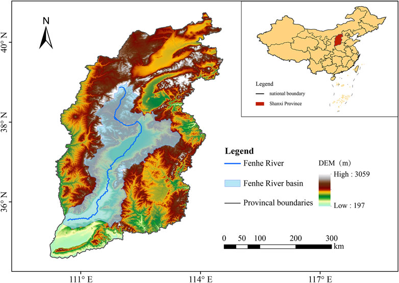
Figure 1. Study area of the FHR Basin, which is located in Shanxi Province. The blue line represents the river, and the shaded part is the basin.

2.2 Data

CN05 is a dataset developed based on 751 meteorological observation stations in China (Xu et al., 2009). The meteorological data used in this experiment are all from the CN05.1 grid dataset, which is produced with reference to the CN05 data and interpolated from more than 2,400 meteorological observation stations in China (Wu and Gao, 2013). The data range from 1961 to 2020, with a spatial resolution of 0.25° × 0.25°. The variables of potential evapotranspiration (PET), vapor pressure deficit (VPD), and the SAPEI were derived from this dataset. All the variables use a daily temporal resolution. Table 1 lists the data used in the study.

Table 1

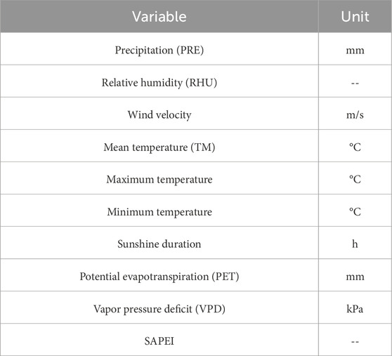
Table 1. CN05.1 data and derived variables.

In the experiment, we set the period from 1961 to 2000 as the training set, 2000 to 2010 as the validation set, and 2011 to 2020 as the test set. We set the duration of the training data to 30 days and the prediction time to 10 days, i.e., 40 days for a sample period. Before the training, we normalized the data from 0 to 1 using the max–min method to speed up the convergence of the model. The calculation is as follows (Equation 1):

${\mathit{X}}_{\mathit{t}}^{*}=\frac{{\mathit{X}}_{\mathit{t}}-{\mathit{X}}^{\mathit{min}}}{{\mathit{X}}^{\mathit{max}}-{\mathit{X}}^{\mathit{min}}},(1)$

where $X_t$ is the grid value of the day t at a certain latitude and longitude, $X^{\mathit{min}}$ is the minimum value of the corresponding latitude and longitude time series, and $X^{\mathit{max}}$ is the maximum value of the corresponding latitude and longitude time series.

2.3 Methodology

2.3.1 SAPEI classification

The SAPEI was used to evaluate the drought degree in the FHR Basin. This index calculation requires PRE and PET data. We choose the Penman–Monteith method to calculate PET, which takes into account various climatic factors such as temperature and humidity and has more physical significance than other methods (Allen et al., 1998; Dai, 2011). The calculation formula of the SAPEI is as follows (Equations 2, 3):

$\mathit{D}={\displaystyle \sum _{\mathit{n}=\mathbf{0}}^{\mathit{N}}}{{\mathit{a}}^{\mathit{n}}\left(\mathit{P}\mathit{R}\mathit{E}-\mathit{P}\mathit{E}\mathit{T}\right)}_{\mathit{n}}.(2)$

${\mathit{a}}^{\mathit{N}}=\mathit{c}.(3)$

In the formula, D represents the daily difference between PRE and PET, a denotes the attenuation constant, N is the number of days ahead, and c denotes the fraction of contribution from the last day of precipitation. Based on previous research, a = 0.98 and c = 13%, resulting in N = 100 (Li et al., 2020; Zhou et al., 2025).

$\mathit{F}\left(\mathit{x}\right)={\left[\mathbf{1}+{\left(\frac{\mathit{\alpha }}{\mathit{x}-\mathit{\gamma }}\right)}^{\mathit{\beta }}\right]}^{-\mathbf{1}},(4)$

$\mathit{S}\mathit{A}\mathit{P}\mathit{E}\mathit{I}=\mathit{w}-\frac{{\mathit{c}}_{\mathbf{0}}+{\mathit{c}}_{\mathbf{1}}\mathit{w}+{\mathit{c}}_{\mathbf{2}}{\mathit{w}}^{\mathbf{2}}}{\mathbf{1}+{\mathit{d}}_{\mathbf{1}}\mathit{w}+{\mathit{d}}_{\mathbf{2}}{\mathit{w}}^{\mathbf{2}}+{\mathit{d}}_{\mathbf{3}}{\mathit{w}}^{\mathbf{3}}}.(5)$

According to the log-logistic distribution, the probability distribution function of the D series is calculated using Equation 4. $\alpha$, $\beta$, and $\gamma$ are the scale, shape, and origin parameters, respectively. If p ≤ 0.5, p = 1-F(x), and $w=\sqrt{-2\mathit{ln}\left(P\right)}$, the value of the SAPEI is calculated according to Equation 5. If p > 0.5, p is replaced by 1-p, and the sign of the SAPEI is reversed. The constants are C₀ = 2.515517, C₁ = 0.802853, C₂ = 0.010328, d₁ = 1.432788, d₂ = 0.189269, and d₃ = 0.001308 (Vicente-Serrano et al., 2010; Wang et al., 2021).

The SAPEI was divided into nine grades according to the severity of drought, namely, extreme wet, severe wet, moderate wet, mild wet, normal, mild drought, moderate drought, severe drought, and extreme drought (Chen et al., 2019; Miah et al., 2017), as shown in Table 2. The study classified the predictions of the models according to drought grades and assessed the predictive performance of the different grades.

Table 2

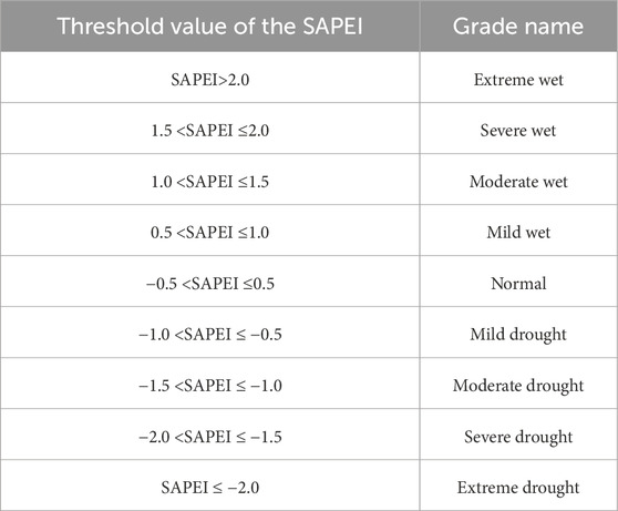
Table 2. Drought severity grades of the SAPEI (Yang et al., 2025).

2.3.2 Models

In this study, we first predict the drought situation in the FHR Basin with a 10-day lead time using five different deep learning models, which are based on the traditional recurrent neural network (RNN) model (Sherstinsky, 2020) and neural network models utilizing the self-attention mechanism. In the traditional model, we choose LSTM, GRU, and biLSTM models, while the neural network based on the self-attention mechanism (Vaswani et al., 2017) uses TFR and IFR models.

RNNs are often used to deal with time-series problems. This concept was proposed by Elman, and the network model used in this study is the LSTM model that evolved from it (Elman, 1990; Hochreiter and Schmidhuber, 1997). This model has a wide range of applications in time-series prediction, such as streamflow prediction and PM_2.5 prediction (Sabzipour et al., 2023; Lin et al., 2024). In the long time-series prediction, the current information is influenced not only by the previous state but also by future information. The biLSTM solves this problem well since it can better capture bidirectional time-series information, and it is widely used in natural language processing and time-series prediction (Kang et al., 2020).

TFR is a sequential model based on attention mechanisms. Different from the traditional RNN, TFR only uses the self-attention mechanism to process the input and output sequences, so it can be calculated in parallel, which greatly improves the computational efficiency. The self-attention mechanism calculates the relationship of each element in the input sequence with all other elements to determinet he corresponding importance of each element. IFR is optimized on the basis of TFR, which effectively reduces the complexity of the TFR model and greatly improves the computational speed of a long time-series (Zhou et al., 2021).

The LSTM model consists of an input layer, an LSTM layer, a fully connected layer, and an output layer. The core architecture of LSTM mainly consists of the forget, input, and output gates. For a time series, the forget gate determines the degree of influence of historical information on the current and future states, that is, the amount of information retained in long-term memory. The input gate determines the information that can be added, while the output gate is responsible for the final output information. BiLSTM is an extension of LSTM. By introducing a bidirectional structure, it can handle both forward and reverse information of time series simultaneously. GRU has been improved on the basis of LSTM by merging the forget and input gates in LSTM into update gates, in which the number of parameters in the model is reduced and the calculation is simpler.

Self-attention-based TFR and IFR are composed of an encoder and a decoder. The encoder processes the time series using multi-head attention, which is calculated independently for each attention head, and then passes the output through a feed-forward neural network. The decoder uses masked multi-head attention to prevent access to future information while generating the prediction for the current time step. Then, the output layer is connected by a feed-forward neural network to obtain the prediction sequence. It is worth noting that the IFR model introduces ProbSparse attention to greatly reduce the computational complexity of the attention mechanism. We used the Adam optimizer, and the number of epochs was set to 100 during training. The batch size of the experiment was set to 32, and the learning rate was 1e-4. The number of heads in multi-head self-attention was set to 8.

2.3.3 Evaluation metrics

In this study, the mean square error (MSE) was used as the index of the loss function of the model. The mean absolute error (MAE) and Pearson correlation coefficient (R) were also selected to evaluate the performance of the model. MSE and MAE were used to represent the gap between the predicted and true values; the smaller the value is, the more accurate the prediction is. R is used to describe the degree of agreement between the predicted and true time series, and a higher value indicates the better prediction performance of the model. The calculation formula of the evaluation index is as follows (Equations 6–9):

$\mathit{M}\mathit{S}\mathit{E}\left({\mathit{y},\mathit{y}}^{\prime }\right)=\frac{{\displaystyle {\sum }_{\mathit{i}=\mathbf{1}}^{\mathit{n}}}{\left({{\mathit{y}}_{\mathit{i}}-\mathit{y}}_{\mathit{i}}^{\prime }\right)}^{\mathbf{2}}}{\mathit{n}},(6)$

$\mathit{M}\mathit{A}\mathit{E}\left({\mathit{y},\mathit{y}}^{\prime }\right)=\frac{\mathbf{1}}{\mathit{n}}{\displaystyle \sum _{\mathit{i}=\mathbf{1}}^{\mathit{n}}}\left|{\mathit{y}}_{\mathit{i}}-{\mathit{y}}_{\mathit{i}}^{\prime }\right|,(7)$

$\mathit{R}\left({\mathit{y},\mathit{y}}^{\prime }\right)=\frac{\mathit{C}\mathit{o}\mathit{v}\left({\mathit{y},\mathit{y}}^{\prime }\right)}{\sqrt{\mathit{V}\mathit{a}\mathit{r}\left[\mathit{y}\right]\mathit{V}\mathit{a}\mathit{r}\left[{\mathit{y}}^{\prime }\right]}},(8)$

$\mathit{B}\mathit{A}\mathit{I}\mathit{S}\left({\mathit{y},\mathit{y}}^{\prime }\right)=\frac{{\displaystyle {\sum }_{\mathit{i}=\mathbf{1}}^{\mathit{n}}}\left({{\mathit{y}}_{\mathit{i}}-\mathit{y}}_{\mathit{i}}^{\prime }\right)}{\mathit{n}}.(9)$

Here, $y_i$ indicates the SAPEI value at the ith day, $y_i^{\prime }$ indicates the predicted value, $Var\left[y\right]\text{\hspace{0.17em}and\hspace{0.17em}}Var\left[y^{\prime }\right]$ denote the variance of the real result and the predicted result, respectively, and $Cov\left({y,y}^{\prime }\right)$ is their covariance.

2.3.4 Interpretability methods

Deep learning models have been widely used in the field of prediction, but in many cases, these are regarded as unexplained black boxes. Thus, understanding how models make accurate predictions is particularly important (Ribeiro et al., 2016). In this study, the SHAP method was used to analyze the contribution degree of different predictors in drought prediction and explore the influence of the predictors on the prediction results under different climatic conditions. SHAP is, therefore, a post-interpretation method. In the SHAP model, each feature is a contribution to the dependent variable, while in drought prediction, different predictors will have an impact on drought (Lundberg and Lee, 2017). SHAP builds the model by calculating the marginal contribution of the features to the model output, and the calculation formula is as follows (Equation 10):

${\mathit{\Phi }}_{\mathit{i}}={\displaystyle \sum _{\mathit{S}\subseteq \mathit{F}\backslash \left\{\mathit{i}\right\}}}\frac{\left|\mathit{S}\right|!\left(\left|\mathit{F}\right|-\left|\mathit{S}\right|-\mathbf{1}\right)!}{\left|\mathit{F}\right|!}\left[{\mathit{f}}_{\mathit{S}\bigcup \left\{\mathit{i}\right\}}\left({\mathit{x}}_{\mathit{S}\bigcup \left\{\mathit{i}\right\}}\right)-{\mathit{f}}_{\mathit{S}}\left({\mathit{x}}_{\mathit{S}}\right)\right],(10)$

where F is the sum of all feature sets; in order to calculate the influence of a feature, $f_{S\bigcup \left\{i\right\}}$ is the training model with the presence of the feature i, $f_S$ is the training model with the feature suppressed, and $x_S$ is the input feature value in the set S.

3 Result

3.1 10-day prediction result

We use MSE to calculate the loss of the model. For different deep learning models, the number of training epochs is uniformly fixed at 100 generations, and the training loss of each model tends to be stable after approximately 30 training cycles. This indicates that the model effectively captures the features within the data, completes the training process, and achieves relatively accurate predictions on the training data. The training situation of the model is shown in Figure 2, where the horizontal axis represents the number of complete passes of the training dataset through the learning algorithm and the vertical axis represents the training loss value. As shown in Figure 2, the convergence time of GRU, LSTM, and biLSTM is slightly longer than that of TFR and IFR. In addition, the training loss values of TFR and IFR are lower than those of GRU, LSTM, and biLSTM, but their training also takes longer. The loss value of each model finally stabilized at approximately 0.01.

Figure 2

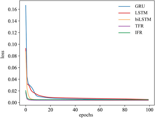
Figure 2. Loss function curves for different models on the training set.

Figure 3 shows the comparison of prediction results from different deep learning models in the test set. When the prediction length is 1 day, we call it PL1, and so on. The MAE values between the predicted and true values of each model increase significantly with an increase in the prediction length. The MAE values of GRU and LSTM are significantly higher than those of biLSTM, TFR, and IFR, indicating that the latter three models perform better than the former two models in drought prediction. In addition, the MAE of the biLSTM model gradually becomes higher than that of TFR and IFR. The increase in the prediction length highlights the long-term forecasting ability of TFR and IFR compared to biLSTM. By calculating the standard deviation for the samples in the test set, we observe that as the prediction length increases, the standard deviation also gradually increases, indicating that the prediction results become relatively unstable. This is reflected in the expanding shaded area in the figure.

Figure 3

Figure 3. MAE of different models from 1- to 10-day predictions. The shaded area indicates the standard deviation.

To further verify the performance of the model, we calculated the R and MSE values between the predicted and true values of the test set for different prediction lengths (as shown in Table 3). Higher R values and lower MSE values indicate more accurate predictions, and the optimal results are bolded in the table. It can be observed that all models predict an R value higher than 0.75 in a 10-day lead time. In the same way, according to the findings demonstrated by MSE, biLSTM has better prediction accuracy than the remaining models in the short term, but as the prediction length increases, the TFR and IFR models have better prediction performance than the biLSTM model. As the prediction length increases, the MSE of the model’s predicted and true values gradually increases, and the prediction results gradually deteriorate. Overall, the prediction results of all five deep learning models show a high level of confidence.

Table 3

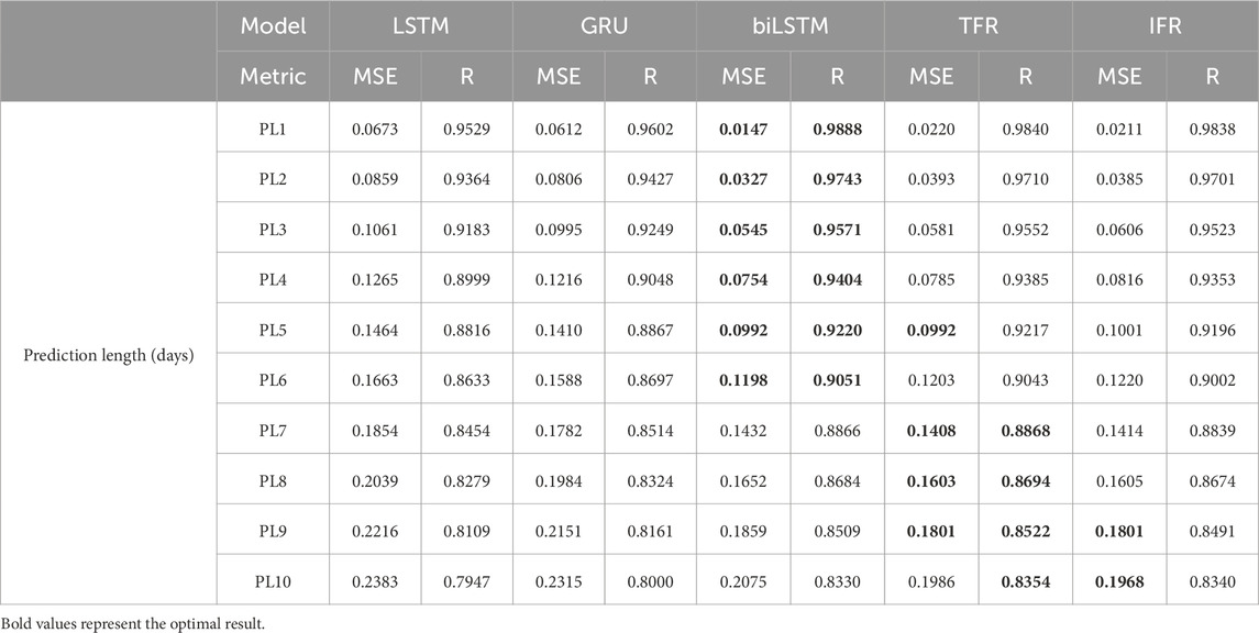
Table 3. Correlation of models at different prediction lengths.

The FHR experienced severe drought and wetting processes in 2011, 2013, and 2019, so we chose these 3 years to check the model’s predictions for the 1-day lead time. The prediction of extreme events provides a better indication of the model’s performance (Camps-Valls et al., 2025). Figure 4 reflects the prediction of drought for the 1-day lead time by three network models in different years. The lines in different colors in the figure indicate different deep learning models, with black representing the SAPEI value. In the first half of the year, the FHR Basin experienced varying degrees of drought, with severe drought conditions particularly in the spring. In the summer of 2013, the area became wet. For these more extreme events, all five models provided relatively accurate predictions, with the green and purple lines aligning more closely with the black line (true value), further confirming the superior performance of the TFR and IFR models. In the spring of 2019, the SAPEI index of the FHR Basin fluctuated greatly, and there was a transition from severe drought to severe humidity in a short period of time. The model also made an accurate prediction for this obvious fluctuation in the short term.

Figure 4

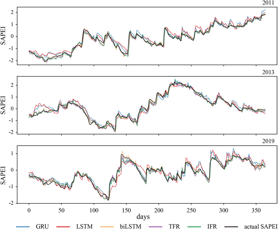
Figure 4. Actual SAPEI values and 1-day predictions of different models in 2011, 2013, and 2019. The black line indicates actual SAPEI values, and the other colored lines indicate 1-day predictions.

Figure 5 reflects the forecast situation of different drought grades. The severity of drought is different, and the prediction difficulty of the model is also different. The extremely small sample content increases the pressure on the training of the model, which also leads to a decrease in the prediction accuracy. Different deep learning models were used to predict the results for the first day of analysis. It should be noted that the SAPEI was divided into nine grades according to relevant studies; however, the samples of the test set did not contain extreme drought values, so only the remaining eight levels were analyzed. It can be observed from the figure that with the aggravation of drought and humidity, the prediction deviation of each model also increases significantly. For humid conditions, the predicted value of the model is often lower than the true value, while for drought conditions, the predicted value of the model is often higher than the true value, which means that the model generally underestimates the humid conditions in the FHR Basin but overestimates the drought conditions in this region. The figure also shows that the prediction deviation of biLSTM, TFR, and IFR in different drought grades is significantly smaller than that of the other two models. However, biLSTM has poor predictions for extreme wet conditions, which indicates the superiority of the TFR and IFR models based on the self-attention mechanism in prediction. This is also consistent with the previous analysis.

Figure 5

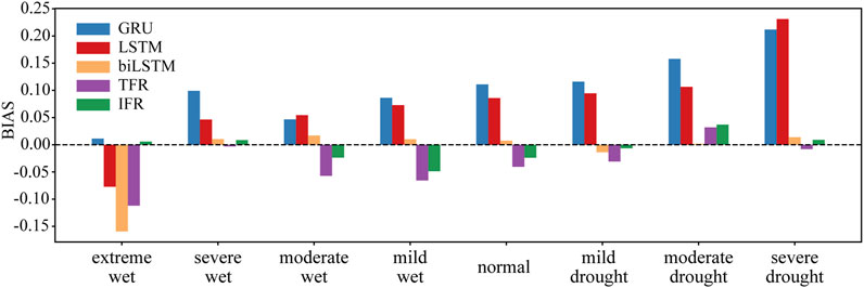
Figure 5. One-day prediction biases of each SAPEI grade with different models.

3.2 Interpretability of 1-day model predictions

Based on the classical LSTM model, this paper further uses the SHAP method to analyze the effects of each variable in predicting the next day. In this process, variables with similar mechanisms were appropriately screened, and the variables used were SAPEI and four auxiliary predictors, namely, temperature (TM), precipitation (PRE), relative humidity (RHU), and potential evapotranspiration (PET). The study used the historical SAPEI value as a predictor to ensure that the experiment was rigorous.

We analyzed the contributions of historical input predictors. In the 1-day prediction (PL1), we also set the sliding window length to 30, so the SHAP method can show the change in the importance of different predictors in the predicting process over the past 30 days. Figures 6a–c show the ranking of the importance of predictors 1-day, 15-day, and 30-day away from the PL1, respectively. The longer the time away from the PL1, the lower the model output value. In different time periods, the importance of predictive factors will vary, but the SAPEI is always the most influential variable. The model most easily captures the change characteristics of the prediction target itself. On the day before PL1, PRE was the most influential variable among the four auxiliary predictors, followed by RHU and PET. With the change in time, the importance of PRE began to decline, while the importance of TM increases significantly. It can be observed that the PRE will affect the drought situation in time, while the TM change in the time period far from the PL1 has a more important impact on the drought. These two changes will comprehensively affect the drought degree (Del-Toro-Guerrero and Kretzschmar, 2020). Wang et al. also showed that PRE plays a leading role in drought occurrence in the Yellow River Basin (Wang et al., 2022). The figure also shows that PET has little influence on drought compared to RHU and PRE. Figure 6d shows the total influence of various variables on PL1 in the past 30 days. Excluding the SAPEI itself, TM is the most influential variable on drought, followed by PRE and RHU, and PET is the weakest.

Figure 6

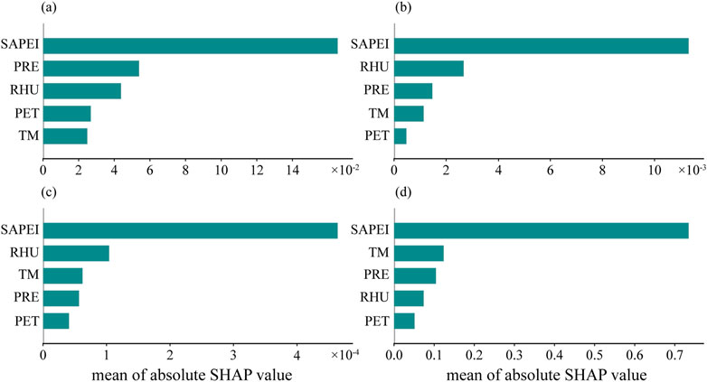
Figure 6. Contributions of predictors in different historical periods; (a–c) 1 day, 15 days, and 30 days away from the forecast target, respectively, and (d) cumulative importance in 30 days.

Figure 7 shows the influence of each variable in the prediction process on the day before PL1 of all samples in the test set. When the SHAP value is positive, it will have a positive impact on the prediction result, and the prediction result will be consistent with the change of the predictor; otherwise, it will have a negative impact, and the change of direction of both will be opposite. The change in color is the change in the value of the predictor itself. It can be observed from the figure that the SAPEI has the strongest influence, which is consistent with previous analysis. With an increase in SHAP values displayed by PRE and RHU, the color of the scatter points gradually deepens, and their values also increase, which is consistent with the physical mechanism. When PRE and RHU increase, the degree of wetting will increase, and the SAPEI will also increase; however, the situation of PET and TM shown in the figure is opposite, i.e., both of them will have a negative impact on the prediction target, and the increase in their own value will aggravate the drought degree and reduce the SAPEI value. The samples with high values are mainly concentrated in the negative region of the SHAP.

Figure 7

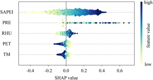
Figure 7. SHAP value of the predictors 1 day before the predicted target; dots indicate dates in the test set. The position of the points on the x-axis indicates the influence of the features on the model, with blue indicating high eigenvalues and yellow indicating low eigenvalues.

In Figure 8, the study analyzed the changes in the importance of all samples in the test set of four auxiliary predictors with their own values. (a)–(d) indicate the total influence of 30 days in history, and the change in color indicates the SAPEI value. As shown in Figure 8a, both high and low temperatures have a great impact on drought. From the distribution of SHAP values, extreme events exist in different seasons. Low TM will lead to a high SHAP value, while high TM corresponds to a low SHAP value, which is mainly caused by the negative influence of TM on the drought index. (b) and (c) correspond to PRE and RHU, respectively. The SHAP value gradually increases as both increase, and the positive impact on the prediction results also gradually increases. High RHU also increases the degree of moistness, which is reflected in the increase in the SAPEI value. This is also consistent with previous analysis. The opposite is true for PET; i.e., when PET increases, it causes drought, and the SAPEI value decreases. Overall, the SHAP method more accurately analyzes the role played by different predictors in the prediction process, thus improving the interpretability principles behind the model while making predictions.

Figure 8

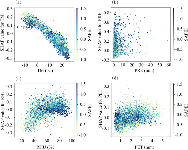
Figure 8. Change of the predictor and its contribution value; the color indicates the SAPEI value. (a–d) represent the four predictors TM, PRE, RHU and PET respectively.

Figure 9 shows the impact of four extreme events on the LSTM model predictions, with two periods of severe wetness and two periods of severe drought chosen as cases for this study. The independent analysis of wet and dry conditions during different periods aims to explain how each meteorological factor affects the prediction results during those times. The two wet periods occurred in the summers of 2013 and 2016, while the drought time periods were mainly concentrated in the springs of 2013 and 2019. The selected sample values for wet periods or droughts were all consistent with a SAPEI value above 1.5 or below −1.5. The figure reflects the total impact of the samples selected for different meteorological factors, where the base value represents the average contribution of all the samples in the test set, and the average contribution of the total samples tends to be 0 due to the large number of samples and the positive and negative impacts on the prediction results. f(x) indicates the weighted contribution of each variable of the selected samples. During the wet period, the blue bar pushes up the contribution of the predicted samples, while the yellow bar decreases the contribution of the predicted samples, and the wider bar indicates the higher contribution, which shows that the SAPEI itself is an important factor influencing the prediction results. Consistent with previous analyses, wet periods had higher PRE and RHU values and SAPEI values greater than 1.5, making the overall impact of the sample positive, while during dry periods, SAPEI values were less than −1.5 and there was relatively less PRE, which reduced the model output.

Figure 9

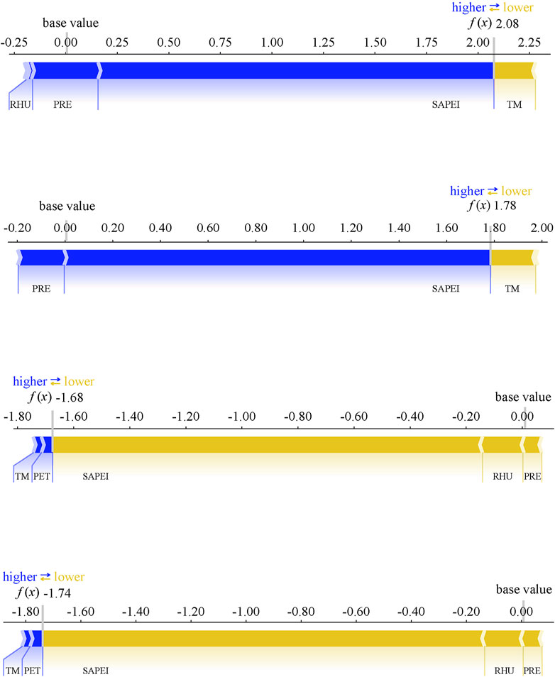
Figure 9. Individual force plots for different drought and wet periods. The base value indicates the average contribution value of the test set data, and f(x) is the contribution value of a certain dry or wet period. Yellow and blue indicate features that push contribution values up and down, respectively.

4 Discussion

4.1 Advantages of the self-attention

TFR is an emerging deep learning model in recent years that has been widely used in the field of prediction, often outperforming previous deep learning methods (Cui et al., 2023; Yang et al., 2023). Our experimental results also indicate that the TFR and IFR models perform better overall. The self-attention in the TFR model can effectively capture the features in the long sequence data, and the LSTM model effectively mitigates the gradient explosion and gradient vanishing problems compared with the traditional recurrent neural network, but its sequential computation still leads to the problem of missing information in the ultra-long sequence data. The self-attention in TFR solves such problems well through the computational principle of parallel operations, but it is highly dependent on a large amount of training data, which also implies higher training costs (Wei et al., 2023). This experiment provides nearly 20,000 training samples to fully utilize the model performance of TFR, which further improves the prediction accuracy.

4.2 Limitations of XAI in this study

This study demonstrates the outstanding performance of deep learning models for drought prediction and assessment. However, balancing the predictive performance of a model with its interpretability is relatively difficult, which requires a combination of effective tools (Jiang et al., 2022). A better understanding of the mechanism behind the model can further improve the model’s performance (Gunning and Aha, 2019).

Predicting extreme events is often difficult, and understanding the impact of meteorological elements during an extreme event has significant research implications. In this study, we used the XAI methods. The SHAP model can analyze the importance of different predictors in the drought prediction process and the different impacts produced by each predictor. However, there are some limitations to this method in the current study, with low computational efficiency being the most obvious. The time required for the SHAP analysis of the predictors is much longer than model training, and the method requires the model to carry out several iterations (van Zyl et al., 2024). In addition, the SHAP model has some limitations in identifying the importance of the predictors, and SAPEI, as the most important variable in the prediction process, accounts for a great proportion of the model’s output, which affects the output of the remaining auxiliary factors to a certain extent and weakens the differences between the factors.

In the historical 30-day predicting cycle, the importance scores of the variables become progressively lower as time increases, and the model is unable to accurately determine the positive and negative feedback effects of the different predictors. The variation in the eigenvalues of each sample with the model output 1-day ahead in Figure 7 is more regular than the total impact shown in Figure 8.

4.3 Importance of short-term drought prediction and future research directions

In this study, a daily drought prediction system was made for the FHR Basin. Unlike the monthly scale long-term prediction, daily drought prediction belongs to the short- and medium-term prediction of drought, which can effectively solve the problem of sudden drought prediction. We cannot ignore the damage caused by short-term droughts. For example, flash droughts can rapidly reduce soil moisture, thereby severely affecting the agricultural economy (Zhang et al., 2023b). Accurate daily forecasting allows the relevant authorities to formulate countermeasures in advance, effectively reducing the damage caused by such disasters.

This experiment mainly focuses on natural factors when considering the factors affecting droughts, which is where our research can be further improved, and the impact of human activities on climate change should not be ignored (Zhang et al., 2023c). Population change and land use type transformation will affect climate change, and in the subsequent research, comprehensive consideration of natural and anthropogenic factors can further clarify the causes of drought, effectively formulate drought mitigation strategies, and improve the accuracy of drought prediction.

5 Conclusion

In this study, we used five different deep learning models, namely, LSTM, GRU, biLSTM, TFR, and IFR, for daily drought prediction in the FHR Basin and evaluated the prediction accuracies and stabilities of the different models under different prediction lengths. In addition, for the classical LSTM model, we re-trained the model to control the prediction length to 1 day and applied deep learning interpretable techniques based on the prediction results to analyze the importance of different predictors in the drought prediction process and how each predictor affects the prediction results. The following conclusions can be drawn from this study:

(1) All five deep learning models performed well in the drought prediction process, and the prediction accuracy decreased with an increase in the prediction duration. The experimental results show that the model performance of biLSTM, TFR, and IFR is significantly better than that of the other two deep learning methods. The TFR and IFR models are more advantageous in long-term prediction. The reason for this result is mainly because the self-attention module in the TFR and IFR models can effectively extract the sample features, thus improving the prediction accuracy of the models. Overall, all five methods provided a more accurate prediction of drought in the FHR Basin in the 10-day lead time.

(2) The SHAP model analyzes the impact of predicting the SAPEI values for the next day with different predictors for 30 days of history, and the experimental results show that the output value of the model decreases with an increase in the length of time from the PL1; in addition, the importance of the predictors changes at different times in the 30 days of history. Among the five different predictors, the SAPEI consistently makes a major contribution, and PRE decreases in importance as the length of time from the PL1 increases, while the importance of TM increases significantly. Combining the total impacts of the 30-day history, TM has a higher impact on the predicted outcomes than PRE and RHU, and PET has the weakest impact on the outcomes.

(3) The experimental results show that different predictors will have different impacts on the prediction results, with the most pronounced performance 1 day prior to the PL1. PRE and RHU will have a positive effect on the predicted values, and the eigenvalues will become larger as the SHAP value increases. The opposite effect is produced by PET and TM; when PET and TM are increased, it will lead to drought, and the SAPEI values will decrease, which will have a negative effect on the predicted results. Combining the historical 30-day model outputs and analyzing the extreme cases lead to the conclusion that the effects of the four auxiliary predictors on drought are consistent with the actual physical mechanisms, with PRE and RHU positively affecting SAPEI values and PET and TM negatively affecting them.

Data availability statement

The original contributions presented in the study are included in the article/supplementary material; further inquiries can be directed to the corresponding author.

Author contributions

ZC: conceptualization, data curation, formal analysis, methodology, software, visualization, and writing – original draft. XW: conceptualization, methodology, supervision, and writing – review and editing. GW: conceptualization, funding acquisition, project administration, supervision, and writing – review and editing. YH: formal analysis and writing – review and editing. HL: formal analysis and writing – review and editing. JZ: writing – review and editing. SZ: writing – review and editing. ZZ: writing – review and editing. YL: writing – review and editing.

Funding

The author(s) declare that financial support was received for the research and/or publication of this article. This work was supported by the National Natural Science Foundation of China (42275028).

Acknowledgments

The authors thank the researchers or teams who provided the basic data. They also thank the authors, reviewers, and editors who made amendments to the article.

Conflict of interest

The authors declare that the research was conducted in the absence of any commercial or financial relationships that could be construed as a potential conflict of interest.

The author(s) declared that they were an editorial board member of Frontiers, at the time of submission. This had no impact on the peer review process and the final decision.

Generative AI statement

The author(s) declare that no Generative AI was used in the creation of this manuscript.

Publisher’s note

All claims expressed in this article are solely those of the authors and do not necessarily represent those of their affiliated organizations, or those of the publisher, the editors and the reviewers. Any product that may be evaluated in this article, or claim that may be made by its manufacturer, is not guaranteed or endorsed by the publisher.

References

Aas, K., Jullum, M., and Løland, A. (2021). Explaining individual predictions when features are dependent: more accurate approximations to Shapley values. Artif. Intell. 298, 103502. doi:10.1016/j.artint.2021.103502

CrossRef Full Text | Google Scholar

Abbes, A. B., Inoubli, R., Rhif, M., and Farah, I. R. (2023). Combining deep learning methods and multi-resolution analysis for drought forecasting modeling. Earth Sci. Inf. 16, 1811–1820. doi:10.1007/s12145-023-01009-4

CrossRef Full Text | Google Scholar

Allen, R. G., Pereira, L. S., Raes, D., and Smith, M. (1998). Crop evapotranspiration-Guidelines for computing crop water requirements-FAO Irrigation and drainage paper 56, 300. Rome: FAO, D05109.

Google Scholar

Camps-Valls, G., Fernández-Torres, M.-Á., Cohrs, K.-H., Höhl, A., Castelletti, A., Pacal, A., et al. (2025). Artificial intelligence for modeling and understanding extreme weather and climate events. Nat. Commun. 16, 1919. doi:10.1038/s41467-025-56573-8

PubMed Abstract | CrossRef Full Text | Google Scholar

Chen, J., Yu, W., Liu, R., Yue, W., and Chen, X. (2019). Daily standardized antecedent precipitation evapotranspiration index (SAPEI) and its adaptability in Anhui Province. Zhongguo Shengtai Nongye Xuebao/Chinese J. Eco-Agriculture 27, 919–928. doi:10.13930/j.cnki.cjea.180835

CrossRef Full Text | Google Scholar

Cho, K., Van Merriënboer, B., Gulcehre, C., Bahdanau, D., Bougares, F., Schwenk, H., et al. (2014). Learning phrase representations using RNN encoder-decoder for statistical machine translation. arXiv Prepr. arXiv:1406.1078. doi:10.3115/v1/D14-1179

CrossRef Full Text | Google Scholar

Cui, B., Liu, M., Li, S., Jin, Z., Zeng, Y., and Lin, X. (2023). Deep learning methods for atmospheric PM2. 5 prediction: a comparative study of transformer and CNN-LSTM-attention. Atmos. Pollut. Res. 14, 101833. doi:10.1016/j.apr.2023.101833

CrossRef Full Text | Google Scholar

Dai, A. (2011). Characteristics and trends in various forms of the palmer drought severity index during 1900–2008. J. Geophys. Res. Atmos. 116, D12115. doi:10.1029/2010jd015541

CrossRef Full Text | Google Scholar

Del-Toro-Guerrero, F. J., and Kretzschmar, T. (2020). Precipitation-temperature variability and drought episodes in northwest Baja California, México. J. Hydrology Regional Stud. 27, 100653. doi:10.1016/j.ejrh.2019.100653

CrossRef Full Text | Google Scholar

Elman, J. L. (1990). Finding structure in time. Cognitive Sci. 14, 179–211. doi:10.1016/0364-0213(90)90002-e

CrossRef Full Text | Google Scholar

Erion, G., Janizek, J. D., Sturmfels, P., Lundberg, S. M., and Lee, S.-I. (2021). Improving performance of deep learning models with axiomatic attribution priors and expected gradients. Nat. Mach. Intell. 3, 620–631. doi:10.1038/s42256-021-00343-w

CrossRef Full Text | Google Scholar

Fang, W., Sha, Y., and Sheng, V. S. (2022). Survey on the application of artificial intelligence in ENSO forecasting. Mathematics 10, 3793. doi:10.3390/math10203793

CrossRef Full Text | Google Scholar

Graves, A., Fernández, S., and Schmidhuber, J. (2005). Bidirectional LSTM networks for improved phoneme classification and recognition. International conference on artificial neural networks. Springer, 799–804.

Google Scholar

Gunning, D., and Aha, D. (2019). DARPA’s explainable artificial intelligence (XAI) program. AI Mag. 40, 44–58. doi:10.1145/3301275.3308446

CrossRef Full Text | Google Scholar

Guo, H., Bao, A., Liu, T., Ndayisaba, F., Jiang, L., Zheng, G., et al. (2019). Determining variable weights for an optimal scaled drought condition index (OSDCI): evaluation in central Asia. Remote Sens. Environ. 231, 111220. doi:10.1016/j.rse.2019.111220

CrossRef Full Text | Google Scholar

Ham, Y.-G., Kim, J.-H., Kim, E.-S., and On, K.-W. (2021). Unified deep learning model for El Niño/Southern Oscillation forecasts by incorporating seasonality in climate data. Sci. Bull. 66, 1358–1366. doi:10.1016/j.scib.2021.03.009

PubMed Abstract | CrossRef Full Text | Google Scholar

Ham, Y.-G., Kim, J.-H., and Luo, J.-J. (2019). Deep learning for multi-year ENSO forecasts. Nature 573, 568–572. doi:10.1038/s41586-019-1559-7

PubMed Abstract | CrossRef Full Text | Google Scholar

Hao, Z., and Singh, V. P. (2015). Drought characterization from a multivariate perspective: a review. J. Hydrology 527, 668–678. doi:10.1016/j.jhydrol.2015.05.031

CrossRef Full Text | Google Scholar

Hochreiter, S., and Schmidhuber, J. (1997). Long short-term memory. Neural Comput. 9, 1735–1780. doi:10.1162/neco.1997.9.8.1735

PubMed Abstract | CrossRef Full Text | Google Scholar

Jia, Y., Zhang, B., and Ma, B. (2018). Daily SPEI reveals long-term change in drought characteristics in Southwest China. Chin. Geogr. Sci. 28, 680–693. doi:10.1007/s11769-018-0973-3

CrossRef Full Text | Google Scholar

Jiang, S., Zheng, Y., Wang, C., and Babovic, V. (2022). Uncovering flooding mechanisms across the contiguous United States through interpretive deep learning on representative catchments. Water Resour. Res. 58, e2021WR030185. doi:10.1029/2021wr030185

CrossRef Full Text | Google Scholar

Kan, J.-C., Ferreira, C. S., Destouni, G., Haozhi, P., Passos, M. V., Barquet, K., et al. (2023). Predicting agricultural drought indicators: ML approaches across wide-ranging climate and land use conditions. Ecol. Indic. 154, 110524. doi:10.1016/j.ecolind.2023.110524

CrossRef Full Text | Google Scholar

Kang, H., Yang, S., Huang, J., and Oh, J. (2020). Time series prediction of wastewater flow rate by bidirectional LSTM deep learning. Int. J. Control 18, 3023–3030. doi:10.1007/s12555-019-0984-6

CrossRef Full Text | Google Scholar

Lamane, H., Mouhir, L., Moussadek, R., Baghdad, B., Kisi, O., and El Bilali, A. (2025). Interpreting machine learning models based on SHAP values in predicting suspended sediment concentration. Int. J. Sediment Res. 40, 91–107. doi:10.1016/j.ijsrc.2024.10.002

CrossRef Full Text | Google Scholar

Lawal, S., Hewitson, B., Egbebiyi, T. S., and Adesuyi, A. (2021). On the suitability of using vegetation indices to monitor the response of Africa's terrestrial ecoregions to drought. Sci. Total Environ. 792, 148282. doi:10.1016/j.scitotenv.2021.148282

PubMed Abstract | CrossRef Full Text | Google Scholar

Lewis, M., Elad, G., Beladev, M., Maor, G., Radinsky, K., Hermann, D., et al. (2021). Comparison of deep learning with traditional models to predict preventable acute care use and spending among heart failure patients. Sci. Rep. 11, 1164. doi:10.1038/s41598-020-80856-3

PubMed Abstract | CrossRef Full Text | Google Scholar

Li, H., Sun, B., Wang, H., Zhou, B., and Duan, M. (2022). Mechanisms and physical-empirical prediction model of concurrent heatwaves and droughts in July–August over northeastern China. J. Hydrology 614, 128535. doi:10.1016/j.jhydrol.2022.128535

CrossRef Full Text | Google Scholar

Li, J., Wang, Z., Wu, X., Xu, C.-Y., Guo, S., and Chen, X. (2020). Toward monitoring short-term droughts using a novel daily scale, standardized antecedent precipitation evapotranspiration index. J. Hydrometeorol. 21, 891–908. doi:10.1175/jhm-d-19-0298.1

CrossRef Full Text | Google Scholar

Lin, M.-D., Liu, P.-Y., Huang, C.-W., and Lin, Y.-H. (2024). The application of strategy based on LSTM for the short-term prediction of PM2. 5 in city. Sci. Total Environ. 906, 167892. doi:10.1016/j.scitotenv.2023.167892

PubMed Abstract | CrossRef Full Text | Google Scholar

Lundberg, S. M., and Lee, S.-I. (2017). A unified approach to interpreting model predictions. Adv. neural Inf. Process. Syst. 30. doi:10.48550/arXiv.1705.07874

CrossRef Full Text | Google Scholar

Miah, M. G., Abdullah, H. M., and Jeong, C. (2017). Exploring standardized precipitation evapotranspiration index for drought assessment in Bangladesh. Environ. Monit. Assess. 189, 547–16. doi:10.1007/s10661-017-6235-5

PubMed Abstract | CrossRef Full Text | Google Scholar

Mishra, A. K., and Singh, V. P. (2010). A review of drought concepts. J. hydrology 391, 202–216. doi:10.1016/j.jhydrol.2010.07.012

CrossRef Full Text | Google Scholar

Palmer, W. C. (1965). Meteorological drought. Weather Bureau: US Department of Commerce.

Google Scholar

Prodhan, F. A., Zhang, J., Hasan, S. S., Sharma, T. P. P., and Mohana, H. P. (2022). A review of machine learning methods for drought hazard monitoring and forecasting: current research trends, challenges, and future research directions. Environ. Model. and Softw. 149, 105327. doi:10.1016/j.envsoft.2022.105327

CrossRef Full Text | Google Scholar

Ribeiro, M. T., Singh, S., and Guestrin, C. (2016). “Why should i trust you? Explaining the predictions of any classifier,” in Proceedings of the 22nd ACM SIGKDD international conference on knowledge discovery and data mining, 1135–1144.

Google Scholar

Sabzipour, B., Arsenault, R., Troin, M., Martel, J.-L., Brissette, F., Brunet, F., et al. (2023). Comparing a long short-term memory (LSTM) neural network with a physically-based hydrological model for streamflow forecasting over a Canadian catchment. J. Hydrology 627, 130380. doi:10.1016/j.jhydrol.2023.130380

CrossRef Full Text | Google Scholar

Selvaraju, R. R., Cogswell, M., Das, A., Vedantam, R., Parikh, D., and Batra, D. (2017). “Grad-cam: visual explanations from deep networks via gradient-based localization,” in Proceedings of the IEEE international conference on computer vision, 618–626.

Google Scholar

Sherstinsky, A. (2020). Fundamentals of recurrent neural network (RNN) and long short-term memory (LSTM) network. Phys. D. Nonlinear Phenom. 404, 132306. doi:10.1016/j.physd.2019.132306

CrossRef Full Text | Google Scholar

Song, Q., Zhao, M.-R., Zhou, X.-H., Xue, Y., and Zheng, Y.-J. (2017). Predicting gastrointestinal infection morbidity based on environmental pollutants: deep learning versus traditional models. Ecol. Indic. 82, 76–81. doi:10.1016/j.ecolind.2017.06.037

CrossRef Full Text | Google Scholar

Song, X., Song, S., Sun, W., Mu, X., Wang, S., Li, J., et al. (2015). Recent changes in extreme precipitation and drought over the Songhua River Basin, China, during 1960–2013. Atmos. Res. 157, 137–152. doi:10.1016/j.atmosres.2015.01.022

CrossRef Full Text | Google Scholar

Sun, J., Liu, Y., Wang, Y., Bao, G., and Sun, B. (2013). Tree-ring based runoff reconstruction of the upper Fenhe River basin, North China, since 1799 AD. Quat. Int. 283, 117–124. doi:10.1016/j.quaint.2012.03.044

CrossRef Full Text | Google Scholar

van Zyl, C., Ye, X., and Naidoo, R. (2024). Harnessing eXplainable artificial intelligence for feature selection in time series energy forecasting: a comparative analysis of Grad-CAM and SHAP. Appl. Energy 353, 122079. doi:10.1016/j.apenergy.2023.122079

CrossRef Full Text | Google Scholar

Vaswani, A., Shazeer, N., Parmar, N., Uszkoreit, J., Jones, L., Gomez, A. N., et al. (2017). Attention is all you need. Adv. Neural Inf. Process. Syst. 30. doi:10.48550/arXiv.1706.03762

CrossRef Full Text | Google Scholar

Vicente-Serrano, S. M., Beguería, S., and López-Moreno, J. I. (2010). A multiscalar drought index sensitive to global warming: the standardized precipitation evapotranspiration index. J. Clim. 23, 1696–1718. doi:10.1175/2009jcli2909.1

CrossRef Full Text | Google Scholar

Wan, L., Bento, V. A., Qu, Y., Qiu, J., Song, H., Zhang, R., et al. (2023). Drought characteristics and dominant factors across China: insights from high-resolution daily SPEI dataset between 1979 and 2018. Sci. Total Environ. 901, 166362. doi:10.1016/j.scitotenv.2023.166362

PubMed Abstract | CrossRef Full Text | Google Scholar

Wang, A., and Ma, X. (2023). An overview of soil moisture drought research in China: progress and perspective. Atmos. Ocean. Sci. Lett. 16, 100297. doi:10.1016/j.aosl.2022.100297

CrossRef Full Text | Google Scholar

Wang, L., and Chen, W. (2014). Applicability analysis of standardized precipitation evapotranspiration index in drought monitoring in China. Plateau Meteorol. 33, 423–431. doi:10.7522/j.issn.1000-0534.2013.00048

CrossRef Full Text | Google Scholar

Wang, T., Tu, X., Singh, V. P., Chen, X., Lin, K., and Zhou, Z. (2023). Drought prediction: insights from the fusion of LSTM and multi-source factors. Sci. Total Environ. 902, 166361. doi:10.1016/j.scitotenv.2023.166361

PubMed Abstract | CrossRef Full Text | Google Scholar

Wang, X., Chen, J., Chen, X., Yue, W., and Wei, Z. (2021). Optimization and applicability analysis of daily farmland drought and flood monitoring index in Huaihe River Basin. Trans. Chin. Soc. Agric. Eng. Trans. CSAE 37, 117–126. doi:10.11975/j.issn.1002-6819.2021.23.014

CrossRef Full Text | Google Scholar

Wang, Y., Wang, S., Zhao, W., and Liu, Y. (2022). The increasing contribution of potential evapotranspiration to severe droughts in the Yellow River basin. J. Hydrology 605, 127310. doi:10.1016/j.jhydrol.2021.127310

CrossRef Full Text | Google Scholar

Wei, X., Wang, G., Schmalz, B., Hagan, D. F. T., and Duan, Z. (2023). Evaluation of Transformer model and Self-Attention mechanism in the Yangtze River basin runoff prediction. J. Hydrology Regional Stud. 47, 101438. doi:10.1016/j.ejrh.2023.101438

CrossRef Full Text | Google Scholar

Wells, N., Goddard, S., and Hayes, M. J. (2004). A self-calibrating Palmer drought severity index. J. Clim. 17, 2335–2351. doi:10.1175/1520-0442(2004)017<2335:aspdsi>2.0.co;2

CrossRef Full Text | Google Scholar

Wu, J., and Gao, X.-J. (2013). A gridded daily observation dataset over China region and comparison with the other datasets. Chin. J. Geophys. 56, 1102–1111. doi:10.6038/cjg20130406

CrossRef Full Text | Google Scholar

Xu, Y., Gao, X., Shen, Y., Xu, C., Shi, Y., and Giorgi, A. (2009). A daily temperature dataset over China and its application in validating a RCM simulation. Adv. Atmos. Sci. 26, 763–772. doi:10.1007/s00376-009-9029-z

CrossRef Full Text | Google Scholar

Xu, Z., Sun, H., Zhang, T., Xu, H., Wu, D., and Gao, J. (2023). Evaluating established deep learning methods in constructing integrated remote sensing drought index: a case study in China. Agric. Water Manag. 286, 108405. doi:10.1016/j.agwat.2023.108405

CrossRef Full Text | Google Scholar

Yang, H., Zhang, Z., Liu, X., and Jing, P. (2023). Monthly-scale hydro-climatic forecasting and climate change impact evaluation based on a novel DCNN-Transformer network. Environ. Res. 236, 116821. doi:10.1016/j.envres.2023.116821

PubMed Abstract | CrossRef Full Text | Google Scholar

Yang, R., Wang, G., Zhang, Y., Zhang, P., Li, S., and Cabral, P. (2025). Cropland exposure to extreme dryness and wetness in China under shared socioeconomic pathways. Int. J. Climatol. 45, e8715. doi:10.1002/joc.8715

CrossRef Full Text | Google Scholar

Yuan, X., Wang, Y., Ji, P., Wu, P., Sheffield, J., and Otkin, J. A. (2023). A global transition to flash droughts under climate change. Science 380, 187–191. doi:10.1126/science.abn6301

PubMed Abstract | CrossRef Full Text | Google Scholar

Zhang, B., Salem, F. K. A., Hayes, M. J., Smith, K. H., Tadesse, T., and Wardlow, B. D. (2023a). Explainable machine learning for the prediction and assessment of complex drought impacts. Sci. Total Environ. 898, 165509. doi:10.1016/j.scitotenv.2023.165509

PubMed Abstract | CrossRef Full Text | Google Scholar

Zhang, Q., Miao, C., Gou, J., and Zheng, H. (2023b). Spatiotemporal characteristics and forecasting of short-term meteorological drought in China. J. Hydrology 624, 129924. doi:10.1016/j.jhydrol.2023.129924

CrossRef Full Text | Google Scholar

Zhang, Q., Miao, C., Guo, X., Gou, J., and Su, T. (2023c). Human activities impact the propagation from meteorological to hydrological drought in the Yellow River Basin, China. J. Hydrology 623, 129752. doi:10.1016/j.jhydrol.2023.129752

CrossRef Full Text | Google Scholar

Zhang, X., Duan, Y., Duan, J., Chen, L., Jian, D., Lv, M., et al. (2022). A daily drought index-based regional drought forecasting using the Global Forecast System model outputs over China. Atmos. Res. 273, 106166. doi:10.1016/j.atmosres.2022.106166

CrossRef Full Text | Google Scholar

Zhou, C., Wang, G., Jiang, H., Li, S., Shi, X., Hu, Y., et al. (2025). Spatio-temporal patterns of compound dry-hot extremes in China. Atmos. Res. 314, 107795. doi:10.1016/j.atmosres.2024.107795

CrossRef Full Text | Google Scholar

Zhou, H., Zhang, S., Peng, J., Zhang, S., Li, J., Xiong, H., et al. (2021). Informer: beyond efficient transformer for long sequence time-series forecasting. Proc. AAAI Conf. Artif. Intell. 35, 11106–11115. doi:10.1609/aaai.v35i12.17325

CrossRef Full Text | Google Scholar