Generation of non-stationary stochastic fields using generative adversarial networks

In the context of geoscience and mineral exploration, accurate characterization of subsurface structures and their spatial variability is crucial for resource evaluation and geoenergy applications, such as hydrocarbon extraction and ${\text{CO}}_2$ storage in deep geological formations. When generating geological facies conditioned on observed data, samples corresponding to all possible spatial configurations are not generally available in the training set. This challenge becomes even greater when dealing with non-stationary fields that exhibit spatially varying statistical properties, which is common in mineral deposits and geological formations. Our study investigates the application of Generative Adversarial Networks (GANs) to generate non-stationary channelized patterns and examines the model’s ability to generalize to unseen spatial configurations not present in the training set. The developed method, based on spatial-conditioning, enables effective learning of the correlation between spatial conditioning data (e.g., non-stationary soft maps) and the generated realizations, without requiring additional loss terms or solving optimization problems for each new data. The models can be trained on both 2D and 3D samples, making them particularly valuable for modeling complex geological structures in mineral deposits. Our results on real and synthetic datasets demonstrate the ability to generate geologically-plausible realizations beyond the training samples with strong correlation to target map. These results underscore the potential of advanced AI techniques to enhance decision-making and operational efficiency in geoenergy projects.

1 Introduction

The generation of stochastic fields has many applications in geosciences and reservoir management. Modeling these fields at the reservoir scale is an essential step in addressing uncertainty quantification or inverse problems in the subsurface. One of the classical approaches is the Multiple Point Statistics (MPS) algorithms (Strebelle, 2002) that were designed for geo-statistical simulation based on spatial patterns in a training image. Many variants of MPS have been developed over time, such as direct sampling techniques (Mariethoz et al., 2010) and cross-correlation based methods (Tahmasebi and Sahimi, 2013). The trained non-parametric model can be used to generate realizations constrained to well and seismic data (Hashemi et al., 2014; Rezaee and Marcotte, 2017; Arpat and Caers, 2007; Tahmasebi et al., 2014). While MPS methods can reconstruct high-dimensional samples from low-dimensional inputs, as demonstrated by (Comunian et al., 2012; Chen et al., 2018; Wang et al., 2022; Guo et al., 2024), they suffer from limitations such as limited variability Emery and Lantuéjoul (2014) and inability to model complex non-stationary patterns (Zhang T. et al., 2019).

Following the success of deep learning in computer vision, recent published work has considered deep generative models such as Generative Adversarial Networks (GANs) (Goodfellow et al., 2014) for generation of stochastic fields. A key advantage of GAN-based approaches over Multiple Point Statistics (MPS) lies in their ability to generate samples with diverse spatial patterns and high-quality reproductions due to the adversarial learning strategy. GANs have been applied to a wide range of geoengineering challenges, including reconstructing the 3D structure of porous media (Mosser et al., 2017), parametrizing high-dimensional spatial permeability fields in the subsurface (Chan and Elsheikh, 2020), and performing geostatistical inversion on both 2D and 3D categorical datasets (Laloy et al., 2018).

GANs have also been used to generate geological realizations conditioned on hard data (e.g., point measurements at wells) and soft data (e.g., probability maps). Approaches for generation of conditioned stochastic realizations could be classified into two categories: post-GANs and concurrent-GANs. In post-GANs approaches, a new optimization problem is solved after training GANs where the latent vector is searched to find realizations that match the target data. For example, the gradient descent method was used in (Dupont et al., 2018; Zhang T. et al., 2019), a Markov chain Monte Carlo sampling algorithm was used (Nesvold and Mukerji, 2019; Laloy et al., 2018), and Chan and Elsheikh (2019) trained an inference network to map the normally distributed outputs to a distribution of latent vectors that satisfies the required conditions. The main drawback of using post-GANs approaches is the additional cost needed to solve the second optimization problem, which can often be expensive. In addition, we would need to solve different problems for every new observed data (e.g., new condition).

In concurrent-GANs approaches, the training of GANs is modified to pass the conditional data to the GANs generator network. After training, the trained generator can then simulate realizations based on the input data without the need to solve another optimization problem. Abdellatif et al. (2022) introduced conditional GANs to generate unrepresented global proportions of geological facies. Cycle-consistent GANs (Zhu et al., 2017) have been used for domain mapping, for example, mapping between physical parameters and model state variables (Sun, 2018) and mapping between seismic data and geological model (Mosser et al., 2018). A GAN model with a U-net architecture (Ronneberger et al., 2015) was used to map high-dimensional input to ${\mathrm{C}\mathrm{O}}_2$ saturation maps (Zhong et al., 2019). However, the one-to-one mapping using Cycle-GANs or U-net architecture is not suitable for generating multiple stochastic facies conditioned on a single observed data.

Song et al. (2021b) used condition-based loss functions to condition facies on hard data and global features, and they later extended the method for spatial probability maps (Song et al., 2021a). Pix2pix method (Isola et al., 2017) has been used for geophysical conditioning by adding additional losses for seismic and well log conditions (Pan et al., 2021). However, condition-based losses require designing manual functions that compute the consistency between the generated samples and target conditions (e.g., computing facies frequency for the generated realizations to mimic real probability maps (Song et al., 2021a)). The design of such function is arbitrary and this is conceptually different than GANs, where the learning is done implicitly from the training data by joint training of both the generator and the discriminator which tells what is good versus bad samples. Moreover, including additional losses in GANs relies on careful weighting between the conditions losses and the original loss in GANs which requires extensive hyper-parameters search (e.g., see Figure 6 in (Song et al., 2021b)).

In this work, we propose a concurrent-GANs approach for generating geological realizations conditioned on spatial maps that describe the distribution of facies proportions across the spatial domain. Notably, this method achieves effective conditioning without relying on explicit condition-based losses. Our approach demonstrates the ability to generate new realizations that align with spatial maps not seen during training, a critical capability for applications where the characteristics of real reservoirs deviate significantly from those of the training data. To incorporate a specific spatial configuration, we employed conditional GANs (cGANs) (Mirza and Osindero, 2014), using spatial maps as input conditions for the neural networks. By integrating the SPADE algorithm (Park et al., 2019), we enabled the generator to dynamically adapt its layers based on the spatial conditioning maps, allowing the GANs to implicitly learn the correlation between the input maps and the generated realizations. The training framework solves a single optimization problem, eliminating the need for designing condition-consistency loss functions or conducting extensive hyperparameter searches for balancing weights. Experimental results on 2D and 3D datasets demonstrate a strong correlation between the generated realizations and the target spatial maps, while also highlighting the model’s ability to generalize to unseen spatial configurations.

The rest of the paper is organized as follows: in Section 2, we discuss the algorithm of conditional GANs used in our experiments and we present the training datasets and the implementation details. In Section 3, the results of the experiments are shown. Finally, conclusions are provided in Section 4.

2 Methods

Generative adversarial networks (GANs) (Goodfellow et al., 2014) are trained to learn the underlying distribution of training samples. It consists of two convolutional neural networks: a generator $G$ and a discriminator $D$. The generator maps a random noise $z$ to a realization $G(z)$ while the discriminator takes samples from the real and the generated sets and is optimized to output the probability of the samples being real (i.e., not generated by the generator). The generator is then optimized such that the generated samples have high probability $D(G(z))$. The two networks are trained in an adversarial setting defined by the objective function $V(G,D)$ in Equation 1:

$\underset{G}{\min }\underset{D}{\max }V\left(G,D\right)={\mathbb{E}}_{x\sim p_x}\left[\log D\left(x\right)\right]+{\mathbb{E}}_{z\sim p_z}\left[\log \left(1-D\left(G\left(z\right)\right)\right)\right].(1)$

Given a spatial map $\mathbf{M}$ that describes the spatial distribution of a geological facies (e.g., channels), we can direct the generated samples to match a particular spatial map $\mathbf{M}$ by using a conditional GANs (Mirza and Osindero, 2014) method, where the condition $\mathbf{M}$ is passed to both the generator network $G$ and discriminator network $D$ during training. Similar to the concurrent-GANs methods, after training we can generate multiple realizations conditioned on $\mathbf{M}$ by simply passing $\mathbf{M}$ and different latent $z$ vectors to the generator without solving a new optimization problem. The discriminator will then output a conditional probability of the sample being real given its input map. The objective function of conditional GANs is defined in Equation 2:

$\underset{G}{min}\underset{D}{max}V\left(G,D\right)={\mathbb{E}}_{x\sim p_x}\left[\log D\left(x|\mathbf{M}\right)\right]+{\mathbb{E}}_{z\sim p_z}\left[\log \left(1-D\left(G\left(z,\mathbf{M}\right)|\mathbf{M}\right)\right)\right].(2)$

To accommodate the spatial nature of the map, we follow the spatially adaptive de-normalization (SPADE) conditioning method developed in (Park et al., 2019), where a segmentation mask modulates the generator layers to generate natural images based on the mask. In our work, we replace the categorical mask with a continuous map that represents the spatial proportions of the channels, these maps are calculated for each sample prior to training. The SPADE method operates as follows: for each layer $i$ and channel $c$ in the generator, the activation $h_{i,c,x,y}$ ($h_{i,c,x,y,z}$ in the case of 3D samples), i.e., the feature produced by a neuron in generator layer $i$, is normalized using the mean ${\mu }_{i,c}$ and standard deviation ${\sigma }_{i,c}$ computed over both batch instances and channel spatial locations. The result is then spatially de-normalized, i.e., adjusted per spatial position, using parameters $\gamma$ and $\beta$, which are learnable functions of $\mathbf{M}$. The calculation of the SPADE algorithm for the 2D case is shown in Equation 3:

${\widehat{h}}_{i,c,x,y}\left(\mathbf{M}\right)={\gamma }_{i,c,x,y}\left(\mathbf{M}\right)\frac{h_{i,c,x,y}-{\mu }_{i,c}}{{\sigma }_{i,c}}+{\beta }_{i,c,x,y}\left(\mathbf{M}\right),\mathbf{M}\in {\mathbb{R}}^{H\times W},(3)$

where the learnable parameters $\gamma$ and $\beta$ are obtained using two successive convolutional layers, separated by a ReLU activation function, directly applied to the map $\mathbf{M}$ and $H\times W$ is the grid dimension at which the channels proportions are calculated.

The spatial proportions of the generated facies can be adjusted by modifying $\mathbf{M}$, which in turn modulates the generator activations through the parameters $\gamma$ and $\beta$. Since each layer of the generator operates at a different resolution, the map $\mathbf{M}$ is dynamically downsampled (or upsampled if $\mathbf{M}$ has a lower resolution) to align with the resolution of the feature maps at each layer. When extending this approach to 3D samples, proportion maps are calculated across all three spatial dimensions. The 3D feature modulation is shown in Equation 4:

${\widehat{h}}_{i,c,x,y,z}\left(\mathbf{M}\right)={\gamma }_{i,c,x,y,z}\left(\mathbf{M}\right)\frac{h_{i,c,x,y,z}-{\mu }_{i,c}}{{\sigma }_{i,c}}+{\beta }_{i,c,x,y,z}\left(\mathbf{M}\right),\mathbf{M}\in {\mathbb{R}}^{H\times W\times D}.(4)$

In the discriminator, features extracted from the map $\mathbf{M}$ using convolutional layers are concatenated with spatial features computed from the input image at an intermediate layer of the network. The intermediate layer is selected so that its resolution matches that of $\mathbf{M}$.

2.1 Implementation details

The generator and discriminator networks are built upon the ResNet architecture (He et al., 2016), following a design approach similar to (Gulrajani et al., 2017). The generator begins by mapping a 128-dimensional noise vector to a hidden representation using a multilayer perceptron (MLP). This hidden representation is then reshaped to dimensions (512, 4, 4), followed by a series of upsampling layers that progressively increase the spatial resolution while reducing the number of feature channels. Conversely, the discriminator performs downsampling operations, halving the spatial resolution and doubling the number of feature channels at each layer. The final output of the discriminator is a single scalar value, representing the probability of the input image being real. We apply spectral normalization to the discriminator’s weights (Miyato et al., 2018) and the self-attention mechanism (Zhang H. et al., 2019) in both the generator and discriminator at an intermediate layer of resolution $32\times 32.$ For all experiments, the models are trained using the Adam optimizer with fixed learning rate of 0.0002 for both networks and a batch-size of 32. The latent vector $z$ is sampled from a multivariate standard normal distribution of dimension 128. The final checkpoint used is based on an exponential moving average of the generator weights with a decaying factor of 0.999 following (Brock et al., 2018). When updating the generator we used $-{\mathbb{E}}_{z\sim p_z}[\log (D(G(z)))]$ as proposed by Goodfellow et al. (2014).

For the 3D model, 3D convolutions, 3D batch-normalization and 3D up-sampling operations are adapted from the PyTorch framework. In this case, the starting vector $z$ is reshaped to $4\times 4\times 2$ and passed to the generator to form $64\times 64\times 32$ 3D images. To handle the size of the 3D samples, our models are trained on four parallel GPUs of GeForce RTX 3090. The architectures of the generator and discriminator networks are depicted in Figures 1, 2, respectively, for simplicity, we removed the self-attention blocks and showed only the 2D models.

Figure 1

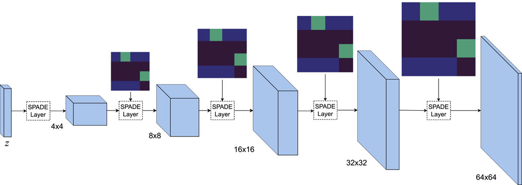
Figure 1. Generator architecture: the stochastic input $z$ is projected through a series of layers to generate an output image, while a conditioning map is introduced at each layer to modulate spatial features adaptively. This modulation is achieved using Spatially-Adaptive Normalization (SPADE) layers, which inject spatially varying information into the generator, ensuring that the output retains structure and fine-grained details. (Park et al., 2019).

Figure 2

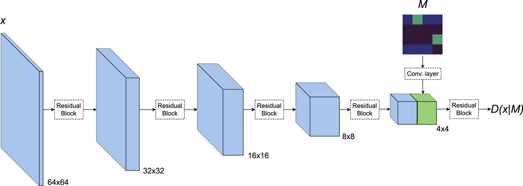
Figure 2. Discriminator architecture: the conditioning map is passed to convolutional layers and the resulting features are concatenated with the input image features (i.e., blue and green features). The discriminator output is the conditional probability of $x$ being real given its corresponding map $\mathbf{M}$.

2.2 Datasets

In our experiments, we evaluate our models on three datasets: a) a 2D synthetic dataset of three facies: channels, levees and background b) a 2D dataset of masks of the Brahmaputra river with binary facies: channels and background and c) a 3D synthetic dataset of binary facies: channels and background. Samples from the 2D datasets are shown in Figure 3. The non-stationarity in the datasets are due to the variations in the channels proportions across the spatial domain, we describe the 2D datasets and the preprocessing steps below.

Figure 3

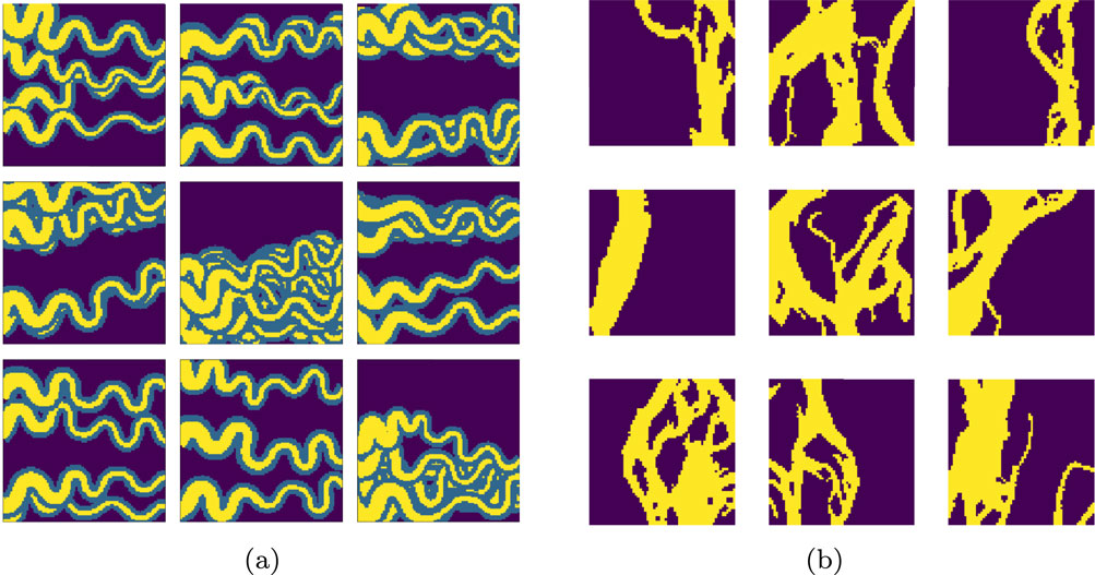
Figure 3. Representative samples from the 2D datasets used for training GAN models: (a) synthetic dataset and (b) real dataset. All images used to train the 2D models are of size $64\times 64$. (a) Artificial dataset of 3 different facies. (b) Binary masks of the Brahmaputra river.

Samples of the first dataset (a) are generated using a geo-modelling tool that mimics depositional environment formation based on random walks (Massonnat, 2019). Horizontal and vertical flipping are performed to increase the sample size from 2,000 to 8,000, this also adds an additional spatial configuration in the training set (i.e., large channel proportion on the right side and low on the left side). The Brahmaputra river mask, dataset (b), is based on the data from Schwenk et al. (2020). The large mask of size $13091\times 11680$ is cropped to patches of size $256\times 256$ with a stride of 64 then the cropped images are rotated such that they have vertical alignment with the central line of the large mask. The central line is computed using RivGraph library (Schwenk et al., 2020). Horizontal and vertical flipping are performed to increase the variations in the training set (increasing sample size from 1788 to 7152). All images of the 2D two datasets are resized to $64\times 64$ resolution to match the networks input.

For each sample in the training set, the channel proportions map $\mathbf{M}$ is calculated at a resolution of $4\times$4 for the 2D samples and $\mathbf{M}\in 4\times 4\times 2$ for the 3D samples. Although they could be calculated at higher resolutions, we chose to mimic the low resolutions usually obtained from seismic surveys. After training, $\mathbf{M}$ can be arbitrary selected to mimic the non-stationarity (e.g., $p\ge 0.4$ is a high proportion and $p\le 0.16$ is a low proportion). While the $4\times$4 grids in our study are abstracted for experimental purposes, they are intended to demonstrate the flexibility of the proposed method to handle diverse input scenarios. In practical geological characterization, the conditioning maps used in this study can be derived or approximated from various data sources. For example, in subsurface modeling, these maps can be constructed from seismic inversion results, which provide spatial distributions of geological properties at different resolutions. Conditioning the generative model on the coarse-scale maps can be used for data assimilation problem of well and flow data as in Fossum et al. (2024).

The 3D dataset (c) is based on data from Sun et al. (2023) and has been used to compare different GANs models (Sun et al., 2021). The original dataset is composed of 25 3D images, of size $256\times 256\times 640$, produced using FLUMY™ computer simulation program and grouped into five groups with different avulsion rates. We selected samples from only the first two groups with low avulsion rates and performed cropping on each image such that the cropped images are of size $64\times 64\times 32$. We use the 3-facies dataset and converted all images to be binary by merging the point bar and channels facies. Finally, flipping is performed to increase the diversity within the dataset. Samples from the dataset are depicted in Figure 4.

Figure 4

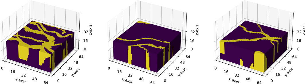
Figure 4. Samples from the 3D training dataset, all images used to train the 3D models are of size $64\times 64\times 32$.

3 Results and discussion

Results on the 2D synthetic dataset and the Brahmaputra river masks are shown in Figures 5, 6, respectively. The leftmost column shows the conditioning maps $\mathbf{M}$, the middle columns are the corresponding generated images $G(z,\mathbf{M})$ and rightmost column shows the mean per pixel maps calculated over 2,000 generated samples. For each row, we used the same conditioning map and different $z$ vectors.

Figure 5

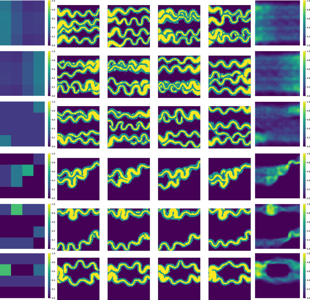
Figure 5. Generated non-stationary realizations on the synthetic dataset: the input conditioning maps are in the leftmost columns, the middle columns are the generated samples and the per-pixel mean maps are in the rightmost columns. The last four rows shows generated samples with maps not seen during training.

Figure 6

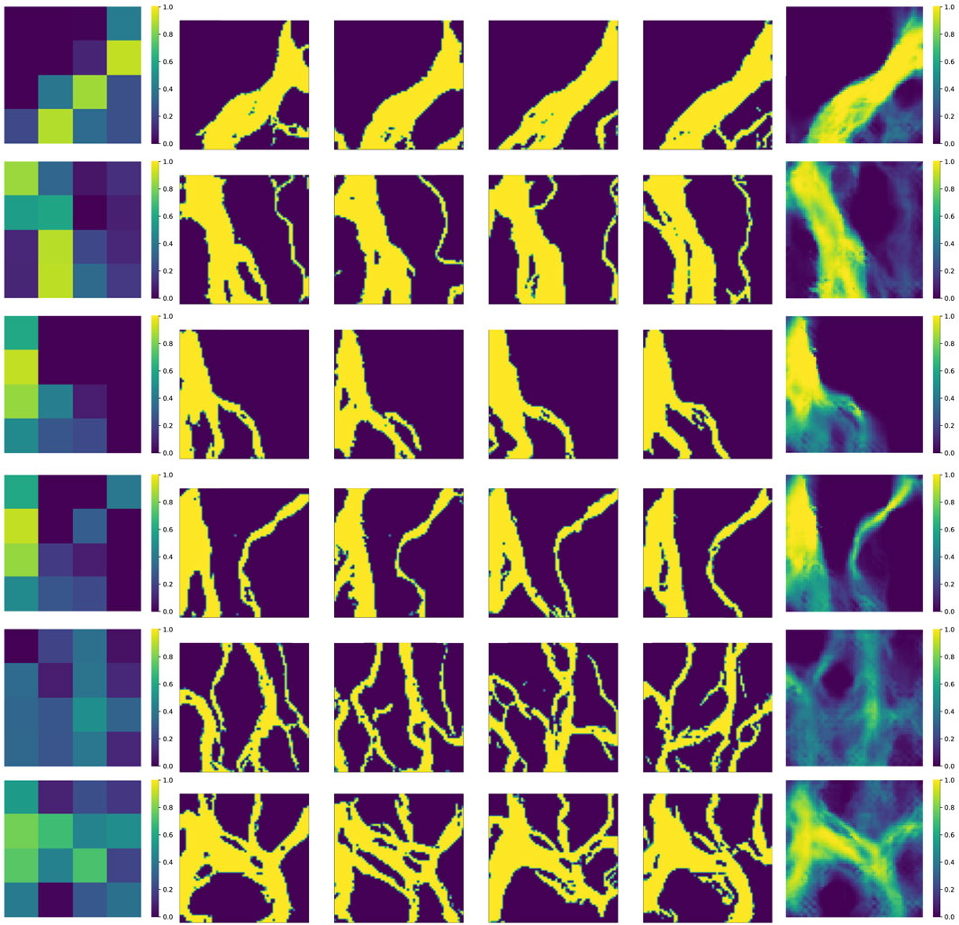
Figure 6. Generated non-stationary realizations on the real masks of the Brahmaputra river: the input conditioning maps are in the leftmost columns, the middle columns are the generated samples and the per-pixel mean maps are in the rightmost columns. The last three rows shows generated samples with maps not seen during training.

In Figure 7, we present the 3D conditional results: in each row, the first column shows the target conditional map $\mathbf{M}$ and the remaining columns show three different generated 3D realizations $x_i=G(z_i,\mathbf{M})$, where each realization is generated with a different $z_i$ and the same map $\mathbf{M}$. From these results, it is clear that our 3D models have learnt a disentangled representation between the $z$ vector which drives the stochastic variation and $\mathbf{M}$ which forces the generated samples to respect the given channel distribution.

Figure 7

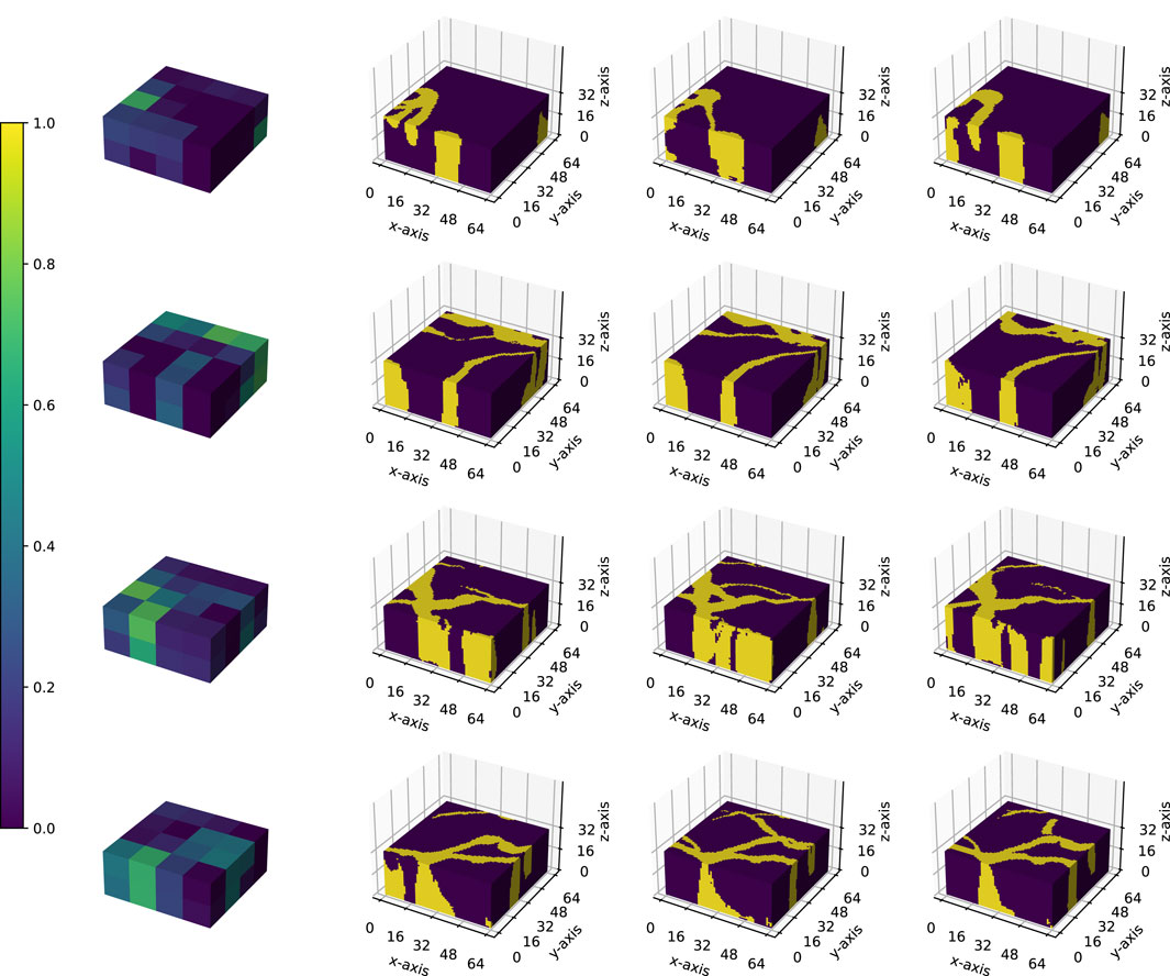
Figure 7. Conditional generated 3D samples. In each row, the first column shows the 3D target map $\mathbf{M}$ and the remaining columns show the generated 3D realization using different random $z$ and the same $\mathbf{M}$. As shown the trained model were able to generate stochastic realizations that matches the target map.

In Figure 8, we present more results of the 3D models at different cross sections. The first two columns show the two sections of the $4\times 4\times 2$ 3D map which describes the target channel proportions for the $64\times 64\times 32$ images across the three dimensions. The remaining columns show generated 2D slices at different cross sections, namely the first, eighth, 16th and 24th. These results demonstrate that the 3D generated samples are spatially-correlated with the target maps in the three dimensions. We note here that although we show results as 2D slices, the 3D images are generated by a single-pass to the generator.

Figure 8

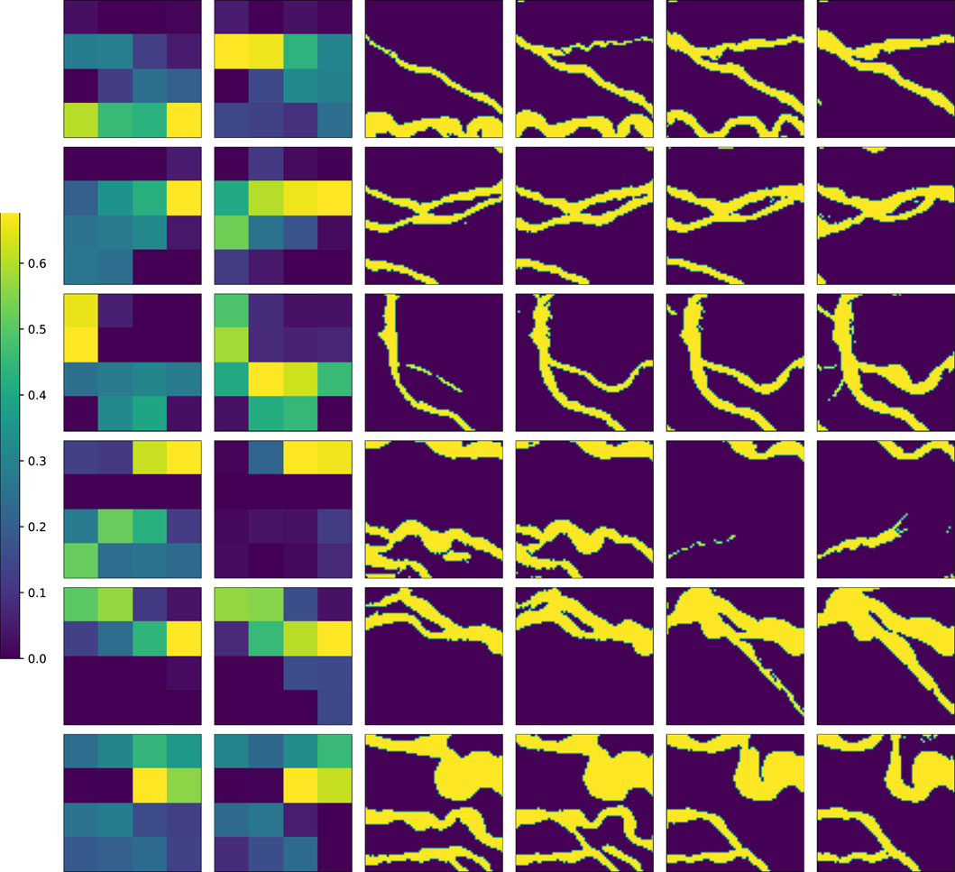
Figure 8. Conditional generated 3D samples with target 3D maps: The first two columns represent the two layers of the $4\times 4\times 2$ target maps, providing the conditioning input. The remaining columns display the corresponding generated 3D sample at different cross-sections, specifically at the first, eighth, 16th, and 24th slices. This visualization highlights how the generated samples align with the spatial structure dictated by the target maps.

The results clearly demonstrate that the models successfully generalized to spatial configurations not present in the training datasets. Visually, the generated samples exhibit geological plausibility; for instance, channel connectivity is preserved across both datasets. Furthermore, in the case of the first dataset, the models consistently generated levees surrounding the channels, regardless of the channels’ locations. This indicates that the models did not simply memorize the training data but instead learned the underlying spatial relationships and patterns effectively.

3.1 Correlation analysis

To quantify the correlation between the target proportion maps and the corresponding generated samples, Figures 9, 10 display $4\times 4$ cross-plots. Each plot corresponds to one section of the $4\times 4$ grid in the conditioning map $\mathbf{M}$. These cross-plots visualize the relationship between the target proportions (x-axis) and the generated proportions (y-axis) for each section, highlighting the model’s ability to replicate local statistics.

Figure 9

Figure 9. A $4\times 4$ grid of cross-plots correlating generated channel proportions with target proportions for individual sections of $4\times 4$ conditioning maps. Each subplot isolates a specific grid section, systematically varying its target proportion while holding others constant. 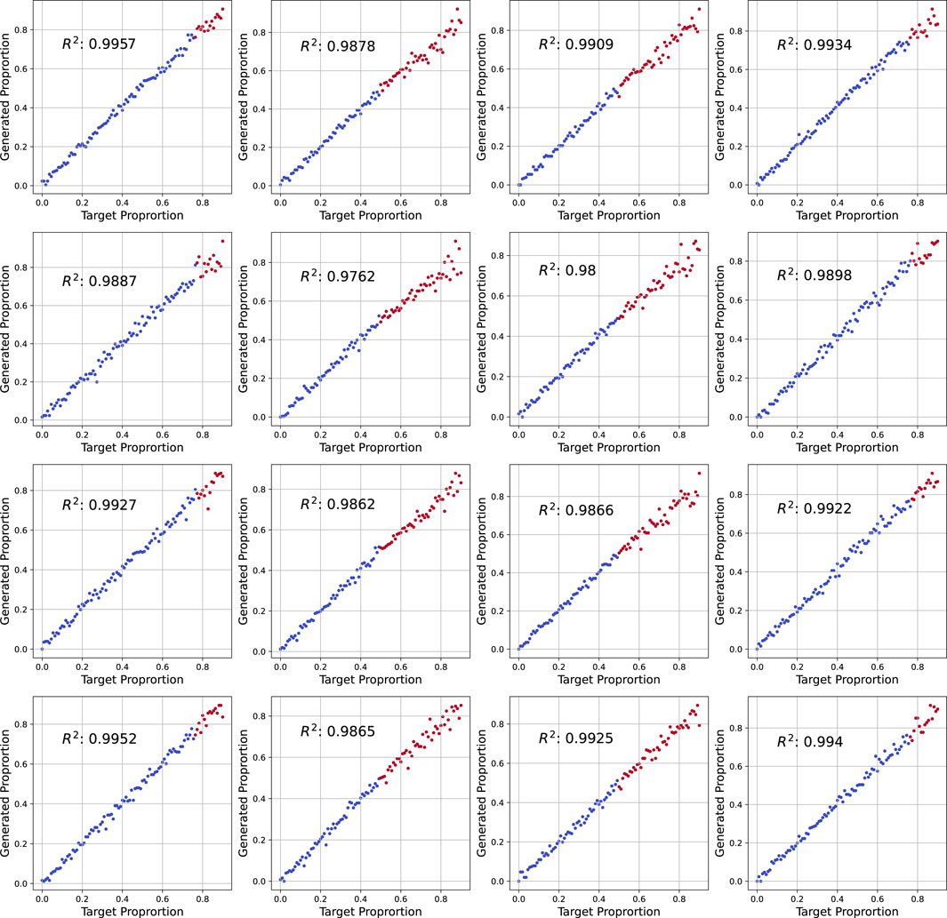Blue markers denote values within the training data distribution, while red markers represent extrapolated proportions outside this range, illustrating the model’s capacity to generalize beyond observed data.

Figure 10

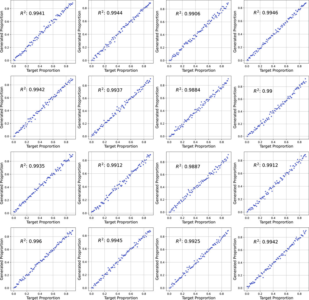
Figure 10. A $4\times 4$ grid of cross-plots correlating generated channel proportions with target proportions for individual sections of $4\times 4$ conditioning maps. Each subplot isolates a specific grid section, systematically varying its target proportion while holding others constant. All points are blue, as the training proportions cover the entire range [0,1].

The results demonstrate a strong correlation between the target and generated proportions, with $R^2$ values approaching 1. This indicates that the model effectively captures the target statistics within each section. Moreover, the model shows the capacity to extrapolate to unseen ranges of proportions. In Figure 9, red dots represent target proportions that lie outside the range observed in the training set, while blue dots represent those within the seen range. The real dataset (Figure 10) spans the entire range [0,1], resulting in all points being blue.

The generalization capability of the GANs can be understood from two perspectives.

1. Local Generalization: The model can generalize to unseen proportions within individual sections of the grid, as illustrated by the red dots in Figure 9.

2. Global Generalization: The model can generate realistic samples for unseen non-stationary configurations across the entire image, as demonstrated in Figures 5, 6.

The two-point probability function quantifies the likelihood that two points, separated by a specified distance, belong to the same channel facies. This measure helps evaluate the spatial continuity and geological consistency of generated samples. In Figure 11, the function is calculated for two specific sections within the $4\times 4$ grid of the 2D datasets: the top-left section and the section in the second row and second column. The analysis is performed under four different conditions to compare the generated samples with the training data. Figures 11a, b present the results for the synthetic dataset, while Figures 11c, d show the results for the real binary masks dataset. Solid lines represent the functions calculated for generated samples, and dashed lines represent those for the corresponding training samples. The results reveal a strong alignment between the generated and training samples, particularly at smaller distances, highlighting the model’s ability to preserve spatial continuity. For unrepresented conditions (e.g., $80\%$ in Figure 11a and $60\%$ and $80\%$ in Figure 11d), the generated functions still follow the general trend of the training data, demonstrating the model’s generalization capacity. At larger distances, some deviations are observed, which may be attributed to the model’s adjustments at boundaries to ensure geological consistency, resulting in differences from the training samples.

Figure 11

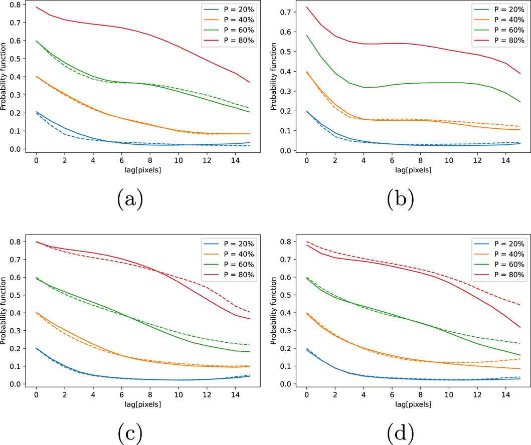
Figure 11. Comparison of two-point probability functions for synthetic and real 2D datasets across distinct grid sections. Subplots (a, b) correspond to synthetic data, while (c, d) represent real binary masks. Dashed lines denote training sample functions at proportions P = {20%,40%,60%,80%}; solid lines show generated samples. The results highlight the alignment between generated and training samples and demonstrate the model’s generalization ability, particularly for unrepresented conditions.

3.2 2D flow simulation

To further assess the trained models, a uniform flow simulation is performed on the training samples shown on left side of Figure 3 and the corresponding generated samples shown on the top row in Figure 5. We consider the problem of a uniform flow where water is injected in order to displace contaminate in a subsurface reservoir. Flow is injected at the left side boundary and produced from the right side boundary and no-flow boundary conditions are imposed on the top and bottom sides. The problem formulation and settings are identical to those presented by Chan and Elsheikh (2020).

We performed a total of 4,000 flow simulations, 2,000 corresponding to the training samples and 2,000 simulations on the GANs generated samples. Flow statistics of the saturation map at $t=0.5$ PVI are shown in Figure 12 for the real and generated samples. As shown, statistics from generated realizations are very similar to the statistics from the training samples. Saturation histograms calculated at the point where the saturation has the highest variance are shown in Figure 13, where the two histograms from the training and generated samples match very well.

Figure 12

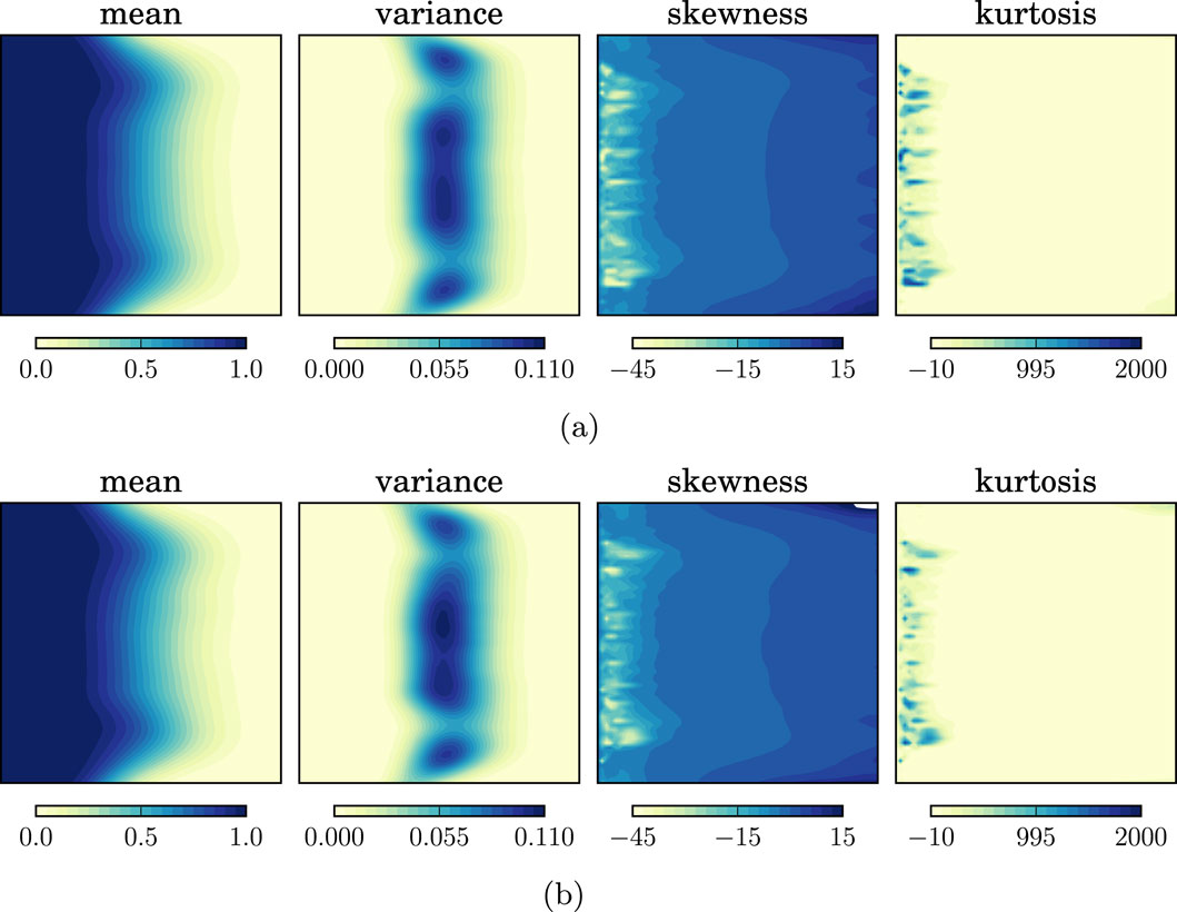
Figure 12. Saturation statistics of a uniform flow on training and generated samples at $t=0.5$ PVI. (a) Statistics on real (i.e.,training) samples. (b) Statistics on generated samples.

Figure 13

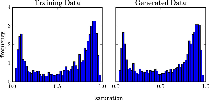
Figure 13. Comparison between training and generated saturation histograms. The histograms display the distribution of saturation values at the spatial location in the domain where the saturation variance is highest, highlighting the range and frequency of saturation fluctuations at that point.

Production curves statistics are shown in Figure 14, where we calculated the mean and the variance of the production curves at different times. We have also plotted the histogram of the water breakthrough time (i.e., the time where the injected clean water level reaches the production well with a 1% threshold). As we can see, the calculated statistics on the generated realizations showed very good agreement with the ones on the training samples which reflect the capabilities of the GANs models.

Figure 14

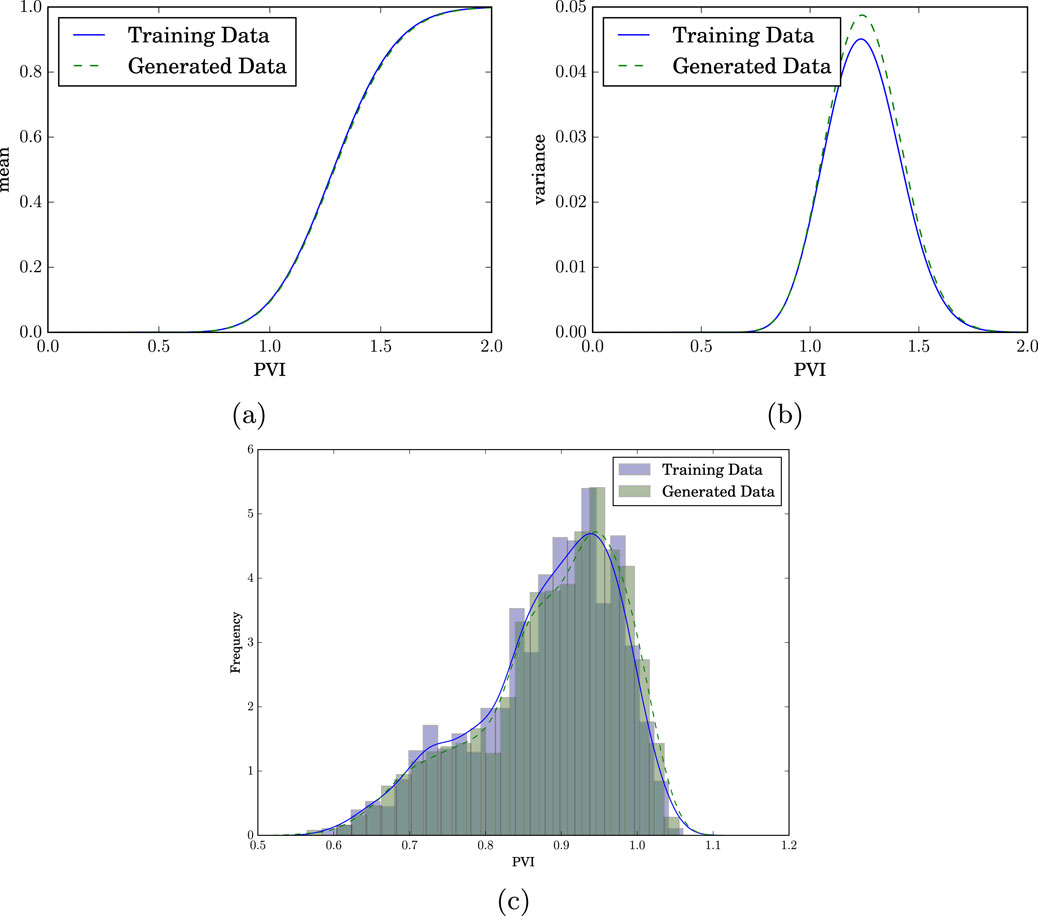
Figure 14. Production Statistics Comparison Between Training and Generated Data (a) Mean production profiles for uniform flow, comparing training data (solid line) and GAN-generated samples (dashed line). (b) Variance distributions of production curves across both datasets. (c) Frequency distribution of water breakthrough times, quantified in pore volume injected (PVI), highlighting discrepancies in temporal dynamics.

4 Conclusion

This study demonstrates that GAN-based methods can effectively generate non-stationary stochastic realizations of geological facies—models that are essential for advanced reservoir characterization in geoenergy applications. The conditioning algorithm allows the model to learn spatial correlations between target maps and generated realizations without solving optimization problems for new observed data or using arbitrary loss functions. Our models consistently produce geologically plausible 2D and 3D realizations, even for spatial configurations not encountered during training, using both synthetic and real geological datasets. This capability is particularly valuable for modeling complex mineral deposits where understanding spatial variability is crucial for resource estimation and development planning. The method’s ability to handle non-stationary fields makes it especially suitable for characterizing heterogeneous geological formations typical in economic geology applications such as hydrocarbon extraction. Future work might include generating non-stationary data from stationary training sets and extending the generated field of view to infinite dimensions.

Data availability statement

The original contributions presented in the study are included in the article/supplementary material, further inquiries can be directed to the corresponding author. The code used to train the GANs models is available on the public repository https://github.com/ai4netzero/NonstationaryGANs.

Author contributions

AA: Conceptualization, Methodology, Software, Writing–original draft, Writing–review and editing. AE: Conceptualization, Funding acquisition, Methodology, Supervision, Validation, Writing–review and editing. DB: Data curation, Resources, Writing–review and editing. PB: Data curation, Resources, Writing–review and editing.

Funding

The author(s) declare that financial support was received for the research and/or publication of this article. This research was partially funded by the Engineering and Physical Sciences Research Council (EPSRC) [Grant No. EP/Y006143/1]. The first author acknowledges financial support from TotalEnergies for his PhD research at Heriot-Watt University. The funder was not involved in the study design, collection, analysis, interpretation of data, the writing of this article, or the decision to submit it for publication.

Conflict of interest

Authors DB and PB were employed by TotalEnergies.

The remaining authors declare that the research was conducted in the absence of any commercial or financial relationships that could be construed as a potential conflict of interest.

Generative AI statement

The author(s) declare that no Generative AI was used in the creation of this manuscript.

Publisher’s note

All claims expressed in this article are solely those of the authors and do not necessarily represent those of their affiliated organizations, or those of the publisher, the editors and the reviewers. Any product that may be evaluated in this article, or claim that may be made by its manufacturer, is not guaranteed or endorsed by the publisher.

References

Abdellatif, A., Elsheikh, A. H., Graham, G., Busby, D., and Berthet, P. (2022). Generating unrepresented proportions of geological facies using generative adversarial networks. Comput. and Geosciences 162, 105085. doi:10.1016/j.cageo.2022.105085

CrossRef Full Text | Google Scholar

Arpat, G. B., and Caers, J. (2007). Conditional simulation with patterns. Math. Geol. 39, 177–203. doi:10.1007/s11004-006-9075-3

CrossRef Full Text | Google Scholar

Brock, A., Donahue, J., and Simonyan, K. (2018). Large scale GAN training for high fidelity natural image synthesis. arXiv. doi:10.48550/arXiv.1809.11096

CrossRef Full Text | Google Scholar

Chan, S., and Elsheikh, A. H. (2019). Parametric generation of conditional geological realizations using generative neural networks. Comput. Geosci. 23, 925–952. doi:10.1007/s10596-019-09850-7

CrossRef Full Text | Google Scholar

Chan, S., and Elsheikh, A. H. (2020). Parametrization of stochastic inputs using generative adversarial networks with application in geology. Front. Water 2 (5). doi:10.3389/frwa.2020.00005

CrossRef Full Text | Google Scholar

Chen, Q., Mariethoz, G., Liu, G., Comunian, A., and Ma, X. (2018). Locality-based 3-d multiple-point statistics reconstruction using 2-d geological cross sections. Hydrology Earth Syst. Sci. 22, 6547–6566. doi:10.5194/hess-22-6547-2018

CrossRef Full Text | Google Scholar

Comunian, A., Renard, P., and Straubhaar, J. (2012). 3D multiple-point statistics simulation using 2D training images. Comput. and Geosciences 40, 49–65. doi:10.1016/j.cageo.2011.07.009

CrossRef Full Text | Google Scholar

Dupont, E., Zhang, T., Tilke, P., Liang, L., and Bailey, W. (2018). Generating realistic geology conditioned on physical measurements with generative adversarial networks. arXiv doi:10.48550/arXiv.1802.03065

CrossRef Full Text | Google Scholar

Emery, X., and Lantuéjoul, C. (2014). Can a training image be a substitute for a random field model? Math. Geosci. 46, 133–147. doi:10.1007/s11004-013-9492-z

CrossRef Full Text | Google Scholar

Fossum, K., Alyaev, S., and Elsheikh, A. H. (2024). Ensemble history-matching workflow using interpretable spade-gan geomodel. First Break 42, 57–63. doi:10.3997/1365-2397.fb2024014

CrossRef Full Text | Google Scholar

Goodfellow, I., Pouget-Abadie, J., Mirza, M., Xu, B., Warde-Farley, D., Ozair, S., et al. (2014). Generative adversarial nets. Adv. Neural Inf. Process. Syst., 2672–2680.

Google Scholar

Gulrajani, I., Ahmed, F., Arjovsky, M., Dumoulin, V., and Courville, A. C. (2017). “Improved training of wasserstein GANs,” in Advances in neural information processing systems, 5767–5777.

Google Scholar

Guo, J., Zheng, Y., Liu, Z., Wang, X., Zhang, J., and Zhang, X. (2024). Pattern-based multiple-point geostatistics for 3d automatic geological modeling of borehole data. Nat. Resour. Res. 34, 149–169. doi:10.1007/s11053-024-10405-6

CrossRef Full Text | Google Scholar

Hashemi, S., Javaherian, A., Ataee-pour, M., Tahmasebi, P., and Khoshdel, H. (2014). Channel characterization using multiple-point geostatistics, neural network, and modern analogy: a case study from a carbonate reservoir, southwest Iran. J. Appl. Geophys. 111, 47–58. doi:10.1016/j.jappgeo.2014.09.015

CrossRef Full Text | Google Scholar

He, K., Zhang, X., Ren, S., and Sun, J. (2016). “Deep residual learning for image recognition,” in Proceedings of the IEEE conference on computer vision and pattern recognition, 770–778.

Google Scholar

Isola, P., Zhu, J.-Y., Zhou, T., and Efros, A. A. (2017). “Image-to-image translation with conditional adversarial networks,” in Proceedings of the IEEE conference onComputer vision and pattern recognition, 1125–1134.

Google Scholar

Laloy, E., Hérault, R., Jacques, D., and Linde, N. (2018). Training-image based geostatistical inversion using a spatial generative adversarial neural network. Water Resour. Res. 54, 381–406. doi:10.1002/2017wr022148

CrossRef Full Text | Google Scholar

Mariethoz, G., Renard, P., and Straubhaar, J. (2010). The direct sampling method to perform multiple-point geostatistical simulations. Water Resour. Res. 46. doi:10.1029/2008WR007621

PubMed Abstract | CrossRef Full Text | Google Scholar

Massonnat, G. (2019). Random walk for simulation of geobodies: a new process-like methodology for reservoir modelling [software]. Pet. Geostat. 2019 2019, 1–5. doi:10.1016/j.cageo.2022.105085

CrossRef Full Text | Google Scholar

Mirza, M., and Osindero, S. (2014). Conditional generative adversarial nets. arXiv Prepr. doi:10.48550/arXiv.1411.1784

CrossRef Full Text | Google Scholar

Miyato, T., Kataoka, T., Koyama, M., and Yoshida, Y. (2018). Spectral normalization for generative adversarial networks. arXiv. doi:10.48550/arXiv.1802.05957

CrossRef Full Text | Google Scholar

Mosser, L., Dubrule, O., and Blunt, M. J. (2017). Reconstruction of three-dimensional porous media using generative adversarial neural networks. Phys. Rev. E 96, 043309. doi:10.1103/physreve.96.043309

PubMed Abstract | CrossRef Full Text | Google Scholar

Mosser, L., Kimman, W., Dramsch, J., Purves, S., De la Fuente Briceño, A., and Ganssle, G. (2018). Rapid seismic domain transfer: seismic velocity inversion and modeling using deep generative neural networks. 80th Eage Conf. Exhib. 2018 2018, 1–5. doi:10.3997/2214-4609.201800734

CrossRef Full Text | Google Scholar

Nesvold, E., and Mukerji, T. (2019). Geomodeling using generative adversarial networks and a database of satellite imagery of modern river deltas. Pet. Geostat. 2019 2019, 1–5. doi:10.3997/2214-4609.201902196

CrossRef Full Text | Google Scholar

Pan, W., Torres-Verdín, C., and Pyrcz, M. J. (2021). Stochastic pix2pix: a new machine learning method for geophysical and well conditioning of rule-based channel reservoir models. Nat. Resour. Res. 30, 1319–1345. doi:10.1007/s11053-020-09778-1

CrossRef Full Text | Google Scholar

Park, T., Liu, M.-Y., Wang, T.-C., and Zhu, J.-Y. (2019). “Semantic image synthesis with spatially-adaptive normalization,” in Proceedings of the IEEE conference on computer vision and pattern recognition, 2337–2346.

Google Scholar

Rezaee, H., and Marcotte, D. (2017). Integration of multiple soft data sets in mps thru multinomial logistic regression: a case study of gas hydrates. Stoch. Environ. Res. Risk Assess. 31, 1727–1745. doi:10.1007/s00477-016-1277-8

CrossRef Full Text | Google Scholar

Ronneberger, O., Fischer, P., and Brox, T. (2015). “U-net: convolutional networks for biomedical image segmentation,” in International conference on Medical image computing and computer-assisted intervention (Springer), 234–241.

Google Scholar

Schwenk, J., Piliouras, A., and Rowland, J. C. (2020). Determining flow directions in river channel networks using planform morphology and topology. Earth Surf. Dyn. 8, 87–102. doi:10.5194/esurf-8-87-2020

CrossRef Full Text | Google Scholar

Song, S., Mukerji, T., and Hou, J. (2021a). Bridging the gap between geophysics and geology with generative adversarial networks. IEEE Trans. Geoscience Remote Sens. 60, 1–11. doi:10.1109/tgrs.2021.3066975

CrossRef Full Text | Google Scholar

Song, S., Mukerji, T., and Hou, J. (2021b). GANSim: conditional facies simulation using an improved progressive growing of generative adversarial networks (GANs). Math. Geosci. 53, 1413–1444. doi:10.1007/s11004-021-09934-0

CrossRef Full Text | Google Scholar

Strebelle, S. (2002). Conditional simulation of complex geological structures using multiple-point statistics. Math. Geol. 34, 1–21. doi:10.1023/a:1014009426274

CrossRef Full Text | Google Scholar

Sun, A. Y. (2018). Discovering state-parameter mappings in subsurface models using generative adversarial networks. Geophys. Res. Lett. 45, 11–137. doi:10.1029/2018gl080404

CrossRef Full Text | Google Scholar

Sun, C., Demyanov, V., and Arnold, D. (2021). Comparison of popular generative adversarial network flavours for fluvial reservoir modelling. 82nd EAGE Annu. Conf. and Exhib. 2021, 1–5. doi:10.3997/2214-4609.202113204

CrossRef Full Text | Google Scholar

Sun, C., Demyanov, V., and Arnold, D. (2023). Gan river-i: a process-based low nt meandering reservoir model dataset for machine learning studies. Data Brief 46, 108785. doi:10.1016/j.dib.2022.108785

PubMed Abstract | CrossRef Full Text | Google Scholar

Tahmasebi, P., and Sahimi, M. (2013). Cross-correlation function for accurate reconstruction of heterogeneous media. Phys. Rev. Lett. 110, 078002. doi:10.1103/physrevlett.110.078002

PubMed Abstract | CrossRef Full Text | Google Scholar

Tahmasebi, P., Sahimi, M., and Caers, J. (2014). Ms-ccsim: accelerating pattern-based geostatistical simulation of categorical variables using a multi-scale search in fourier space. Comput. and Geosciences 67, 75–88. doi:10.1016/j.cageo.2014.03.009

CrossRef Full Text | Google Scholar

Wang, L., Yin, Y., Zhang, C., Feng, W., Li, G., Chen, Q., et al. (2022). A mps-based novel method of reconstructing 3d reservoir models from 2d images using seismic constraints. J. Petroleum Sci. Eng. 209, 109974. doi:10.1016/j.petrol.2021.109974

CrossRef Full Text | Google Scholar

Zhang, H., Goodfellow, I., Metaxas, D., and Odena, A. (2019a). “Self-attention generative adversarial networks,” in International conference on machine learning, 7354–7363.

Google Scholar

Zhang, T., Tilke, P., Dupont, E., Zhu, L., Liang, L., and Bailey, W. (2019b). “Generating geologically realistic 3d reservoir facies models using deep learning of sedimentary architecture with generative adversarial networks,” in International petroleum technology conference (OnePetro).

Google Scholar

Zhong, Z., Sun, A. Y., and Jeong, H. (2019). Predicting CO₂ plume migration in heterogeneous formations using conditional deep convolutional generative adversarial network. Water Resour. Res. 55, 5830–5851. doi:10.1029/2018wr024592

CrossRef Full Text | Google Scholar

Zhu, J.-Y., Park, T., Isola, P., and Efros, A. A. (2017). “Unpaired image-to-image translation using cycle-consistent adversarial networks,” in Proceedings of the IEEE international conference on computer vision, 2223–2232.

Google Scholar