Automatic seismic-well tie based on cascaded matching optimization method

Seismic-well tie, the alignment of synthetic traces with actual seismic traces at well locations, is a fundamental step in seismic interpretation, inversion, and reservoir prediction. This process involves multiple steps, including preprocessing well logs, calculating reflection coefficients, wavelet estimation, synthetic traces generation, and aligning synthetic traces with seismic data. This study focuses on the automated matching process, addressing its challenges and improving accuracy. Existing methods, such as correlation-based approaches, local similarity scan, and dynamic time warping, face limitations in handling time-varying shifts. To overcome these challenges, we propose the cascaded matching optimization method. This method decomposes the time shifts calculation into two steps: first, smooth time shifts are determined using local similarity scan while preserving waveform characteristics to perform an initial correction; second, the corrected synthetic trace is refined to account for residual shifts. Tests using synthetic and field data demonstrate that this method achieves accurate automatic seismic-well tie while preserving waveform fidelity.

1 Introduction

Well log curves can provide detailed subsurface parameters and geological interface stratigraphy, and are often used in conjunction with seismic data, offering high vertical resolution. However, since most seismic data are in the time domain, while well log data are in the depth domain, it is necessary to correlate well and seismic data. This process is referred to as “seismic-well tie.” Seismic-well tie is tying the synthetic trace to the actual seismic trace at the well location, which is the most fundamental and crucial step in seismic data interpretation (El Dally et al., 2023), inversion (Wo et al., 2025), and subsequent reservoir prediction (White and Simm, 2003).

Seismic-well tie is typically conducted in the time domain. The basic process of seismic-well tie involves five steps: (1) Preprocessing of well logging data. Logging data is affected by factors such as borehole enlargement and mud invasion, resulting in local anomalies. It is necessary to reconstruct the abnormal segments or use filtering methods for processing (Duchesne and Gaillot, 2011). (2) Calculation of reflection coefficients through velocity log and density log. It is important to note that, due to the convolution with the wavelet required in the subsequent steps, what is needed is a time-domain reflectivity sequence. Whether calculating the reflectivity sequence using impedance sequences in the depth domain and then converting it to the time domain, or first transforming the impedance sequence to the time domain and then calculating the reflectivity sequence, there are differences in the synthetics generated by these two methods (Anderson and Newrick, 2008). (3) Estimation of appropriate seismic wavelets. (4) Convolution of reflection coefficients with seismic wavelets to generate a synthetic trace. Due to factors such as anelastic attenuation (including anisotropy attenuation), interbed multiples, the wavelet undergoes variations in both space and time (van der Baan, 2008). However, the wavelet is a critical factor when generating the synthetic trace (Munoz and Hale, 2012). (5) Bulk shifting and appropriate stretching or compression of the synthetic trace to tie seismic data at the well location. This series of steps does not seem very difficult, so many details within it are easily overlooked, resulting in poor quality of the seismic-well tie.

In this paper, we focus on the fifth step, assuming that the first four steps have already been completed and are reasonable. As exploration progresses, the number of wells continues to increase, and in areas with high-density well networks, the manual search by interpreters for the best match between the seismic trace near the well and the synthetic trace in step five becomes an extremely time-consuming task. Currently, the methods commonly used for automatic seismic-well tie matching can be roughly divided into three categories. The first category is based on correlation coefficients. By calculating the cross-correlation between the seismic and well traces, the global correlation coefficient can be obtained, and the time shifts corresponding to the maximum global correlation can be used to apply a bulk shift to the synthetic trace, thereby achieving the seismic-well tie. The time shifts between the seismic and well traces are necessarily time-varying due to factors such as frequency-dependent attenuation that causes velocity differences between well logs and seismic data (Cui, 2015), as well as the mismatch between the synthetic wavelet used for convolution and the actual seismic wavelet (Santos et al., 2024). The local cross-correlation algorithm (Hale, 2006; Hale, 2009) introduces a Gaussian window function during the cross-correlation calculation, dividing the seismic and synthetic traces into multiple local signals. By calculating the correlation coefficients between these local signals, a time-varying displacement sequence can be obtained. This method is theoretically straightforward and easy to implement. However, the choice of window size is crucial. If the local signals exhibit significant variation, a narrower time window is required, which can reduce the stability of the results. Conversely, increasing the window size to improve stability may reduce the accuracy of the calculated time shifts. To overcome these limitations, Fomel (2007a); Fomel and Jin (2009) proposed the concept of local similarity, which involves calculating the similarity characteristics within the local neighborhood of each sampling point using least-squares inversion. This process is then used to further derive the time shifts. Local similarity, compared to local cross-correlation, does not heavily rely on window selection and can calculate smooth time shifts (Herrera et al., 2014) enabling appropriate stretching and compression of synthetic traces to achieve seismic-well tie. The second category is based on dynamic time warping (DTW). An early approach to DTW was introduced by Martinson and Hopper (1992) Martinson et al. (1982). Herrera and van der Baan (2012) applied DTW for the automatic alignment of well and seismic traces. More recently, Hale (2013) improved DTW by incorporating time shifts directly into the algorithm. Furthermore, Herrera and van der Baan (2014) introduced global constraints to ensure that the maximum amount of stretching and compression remains within a reasonable range. The third and most recent category involves artificial intelligence (AI)-based methods. Wu et al. (2022) proposed an automatic well-seismic tie algorithm that combines convolutional neural networks (CNN) with variable window resampling. However, the stretch range of the variable window significantly affects the quality of the training dataset. Di and Abubakar (2023) applied self-supervised learning to seismic-well tie, which enables the automatic extraction of features from unlabeled data, thereby reducing the need for manual labeling. Additionally, Santos et al. (2024) developed a deep learning model based on a multilayer perceptron (MLP) neural network, which predicts accurate wavelets using only seismic traces. This AI-predicted wavelet is then used to generate synthetic traces that better match the observed seismic data, effectively enhancing the seismic-well tie quality.

Through a review of existing literature and technologies, it is found that automatic seismic-well tie methods based on local similarity scan (LSS) and DTW still exhibit certain limitations. In response, we propose a novel automatic seismic-well tie method based on cascaded matching optimization (CMO). We normalize this local similarity attribute, LSS to compute the smooth time shifts, aligning the major waveform features of the synthetic seismogram and the nearby seismic trace while preserving the waveform characteristics. This step provides an optimized synthetic trace as input for subsequent DTW-based residual time shifts calculation. The synthetic trace is then further refined to enhance well-seismic consistency. This paper is organized as follows: first, the principles of the LSS and DTW methods are introduced, and their limitations are demonstrated using the synthetic data. Then, the cascaded matching optimization method is applied for the automatic seismic-well tie of both synthetic and field data. The seismic-well tie’s results are quality-controlled using three approaches: multi-well time-depth relationships, well-tie profiles, and well-seismic correlation coefficients. All results indicate that the proposed method achieves satisfactory outcomes.

2 Methodology

2.1 Local similarity scan

The global correlation coefficient $r$ is a statistical measure used to quantify the degree of linear correlation between two signals, x and y, with a value ranging between −1 and 1. The formula for calculating the coefficient $r$ is defined as Equation 1:

$r=\frac{{\displaystyle {\sum }_{t=1}^N}x\left(t\right)\mathrm{y}\left(t\right)}{\sqrt{\left[{\displaystyle {\sum }_{t=1}^N}x\left(t\right)x\left(t\right)\right]\left[{\displaystyle {\sum }_{t=1}^N}\mathrm{y}\left(t\right)y\left(t\right)\right]}},(1)$

In the formula, t denotes the time sample index, and N represents the total number of samples in the signal. The squared global correlation coefficient can be expressed as the product of two components, as shown in Equation 2:

$r^2=r_1{r}_2.(2)$

Here, $r_1$ and $r_2$ represent the components related to the two signals, which can be expressed as follows:

$r_1=\frac{{\displaystyle {\sum }_{t=1}^N}x\left(t\right)y\left(t\right)}{\sqrt{{\displaystyle {\sum }_{t=1}^N}{\left[x\left(t\right)\right]}^2}}={\left({\mathbf{x}}^T\mathbf{x}\right)}^{-1}\left({\mathbf{x}}^T\mathbf{y}\right),(3)$

$r_2=\frac{{\displaystyle {\sum }_{t=1}^N}x\left(t\right)y\left(t\right)}{\sqrt{{\displaystyle {\sum }_{t=1}^N}{\left[\mathrm{y}\left(t\right)\right]}^2}}={\left({\mathbf{y}}^T\mathbf{y}\right)}^{-1}\left({\mathbf{y}}^T\mathbf{x}\right).(4)$

In Equations 3, 4, $\mathbf{x}$ is a vector notation for $x\left(t\right)$, and $\mathbf{y}$ is a vector notation for $y\left(t\right)$ , where the superscript ${\left(\right)}^T$ denotes the transpose.

To compute the local similarity at each sample point between two signals, we first convert them into diagonal operators: $\mathbf{X}$ is a diagonal operator composed from the elements of x, and $\mathbf{Y}$ is a diagonal operator composed from the elements of y. Then, we introduce a regularization operator $\mathbf{R}$, specifically the shaping regularization operator (Fomel, 2007b), to localize the least-squares inversion. This effectively smooths the results and ensures stability during the iterative solution. The local similarity components $r_1\left(t\right)$ and $r_2\left(t\right)$ can then be computed as shown in Equations 5, 6:

$r_1\left(t\right)=\left[{\mu }^2\mathbf{I}+\mathbf{R}{\left({\mathbf{X}}^T\mathbf{X}-{\mu }^2\mathbf{I}\right)}^{-1}\right]\mathbf{R}{\mathbf{X}}^T\mathbf{y}(5)$

$r_2\left(t\right)=\left[{\mu }^2\mathbf{I}+\mathbf{R}{\left({\mathbf{Y}}^T\mathbf{Y}-{\mu }^2\mathbf{I}\right)}^{-1}\right]\mathbf{R}{\mathbf{Y}}^T\mathbf{x}(6)$

Here, $\mu$ is a scaling parameter used to balance the identity operator $\mathbf{I}$ and the signal energy term in the shaping regularization. The result of local similarity $c\left(t\right)$ is the product of $r_1\left(t\right)$ and $r_2\left(t\right)$. By introducing different time shifts l into the signal x, we perform the calculation of local similarity, ultimately obtaining a spectrum of local similarity coefficients $c\left(t,l\right)$.

Hereafter, it is necessary to pick the time shifts ${\tau }_1\left(t\right)$ for each sampling point from the local similarity spectrum $c\left(t,l\right)$. The traditional method involves traversing each sampling point and selecting the value of $l$ where the similarity is maximized. However, this method may lead to discontinuous or unstable picking trajectories. In this paper, a novel automatic picking method is employed, viewing the similarity picking process as a variational problem (Fomel, 2009), analogous to the ray tracing problem-just as the first-arrival seismic ray corresponds to the trajectory with the minimum travel time. The optimal similarity trend ${\tau }_1\left(t\right)$ should minimize the path defined in Equation 7:

$path\left[{\tau }_1\left(t\right)\right]={\displaystyle \underset{t_{\min }}{\overset{t_{\max }}{\int }}}{e}^{\left[-c\left(t,{\tau }_1\left(t\right)\right)\right]\sqrt{{\lambda }^2+\left[{\tau }_1^{\prime }{\left(t\right)}^2\right]}}dt.(7)$

where $\lambda$ is a scaling parameter controlling the smoothness of the trajectory. According to variational theory, this leads to the following eikonal-type equation, as shown in Equation 8:

${\left(\frac{\mathrm{\partial }T}{\mathrm{\partial }{\tau }_1}\right)}^2+\frac{1}{{\lambda }^2}{\left(\frac{\mathrm{\partial }T}{\mathrm{\partial }t}\right)}^2=e^{-2c\left(t,{\tau }_1\left(t\right)\right)}.(8)$

where $T\left(t,l\right)$ denotes the accumulated traveltime-like cost function. In this analogy, the local similarity $c\left(t,l\right)$ plays the role of inverse velocity (i.e., squared slowness), and regions of high similarity act as “waveguides” that attract the optimal trajectory. The final picking path ${\tau }_1\left(t\right)$ is extracted by backward ray tracing along the gradient of $T\left(t,l\right)$, and smoothed using shaping regularization (Fomel, 2007b), to suppress random oscillations.

2.2 Dynamic time warping

DTW is an effective tool for measuring the similarity between two sequences. It works by calculating the Euclidean distance between each pair of sampling points in the two sequences, constructing a Euclidean distance matrix, and then using dynamic programming to accumulate and sum the Euclidean distances, forming a cumulative Euclidean distance matrix. Finally, a backtracking process is used to determine the matching relationship between sampling points in the two sequences.

If we denote the seismic trace near the well as $y\left(t\right)$ and the synthetic trace as $x\left(t\right)$, traditional DTW requires computing the Euclidean distance matrix by comparing every sample point in $y\left(t\right)$ with every sample point in $x\left(t\right)$. This results in a large computational cost and is inconsistent with physical principles, as the synthetic trace cannot realistically undergo such extreme stretching and compression. To address this, Hale (2013) introduced a time-window constraint, meaning that when calculating the Euclidean distance matrix (also referred to as the error matrix $e_{t,l}$ here), each sample point in $y\left(t\right)$ is only compared to sample points within a certain neighborhood in $x\left(t\right)$. The Euclidean distance is calculated based on the amplitude differences at each sampling point, using the following formula:

$e_{t,l}={\left[y\left(t\right)-x\left(t+l\right)\right]}^2.(9)$

Equation 9 quantifies the local errors of each sampling point of the two sequences. To find an optimal matching path, it is necessary to minimize the global error. First, initialize the first column of the global error matrix, as shown in Equation 10:

${\gamma }_{1,l}=e_{1,l}.(10)$

Then cumulative error matrix ${\gamma }_{t,l}$ can be achieved by accumulating errors through the following method:

${\gamma }_{t,l}=e_{t,l}+\min \left\{\begin{array}{l}{\gamma }_{t-1,l-1}\\ {\gamma }_{t-1,l}\\ {\gamma }_{t-1,l+1}\end{array}\right..(11)$

Equation 11 is illustrated in Figure 1a. At each point, the accumulated error is computed by comparing the cumulative errors from the three preceding directions, selecting the minimum among them, and adding the current local error to obtain the cumulative error at the current position.

Figure 1

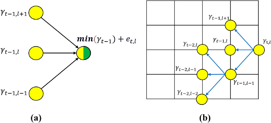
Figure 1. (a) Schematic diagram of the DTW cumulative error matrix calculation; (b) Schematic diagram of the DTW path backtracking.

Finally, we find the point with the smallest global error value from the last column of the global error matrix, which serves as the starting point for backtracking the path. The corresponding time shift l for this minimum value is stored as the last element in the one-dimensional sequence ${\tau }_2\left(t\right)$as shown in Equation 12:

${\tau }_2\left(N\right)=\underset{l}{\mathrm{argmin}}\left({\gamma }_{N,l}\right).(12)$

Since the error accumulation is based only on the global error values from the previous three points (${\gamma }_{t+1,{\tau }_2\left(t+1\right)-1},{\gamma }_{t+1,{\tau }_2\left(t+1\right)},{\gamma }_{t+1,{\tau }_2\left(t+1\right)+1}$), we determine the minimum among these three global error values and record the corresponding time shift l, storing it in the sequence ${\tau }_2\left(t\right)$. This recursive processing continues using the following formula:

${\tau }_2\left(t\right)=\underset{l}{\mathrm{argmin}}\left\{\begin{array}{l}{\gamma }_{t+1,{\tau }_2\left(t+1\right)-1}\\ {\gamma }_{t+1,{\tau }_2\left(t+1\right)}\\ {\gamma }_{t+1,{\tau }_2\left(t+1\right)+1}\end{array}\right.,t=N-1,......,1.(13)$

Equation 13 is conceptually illustrated in Figure 1b. During the backtracking procedure, the cumulative error at the current point is assumed to originate from one of the three adjacent directions. Accordingly, the cumulative errors from these directions are evaluated, and the direction associated with the minimum cumulative error is selected. This process is iteratively applied to trace back the optimal alignment path.

2.3 Cascaded matching optimization method

Let the seismic trace recorded near the well be denoted as $y\left(t\right)$, and the synthetic trace generated from well log data be denoted as $x\left(t\right)$. During the seismic-well tie, the synthetic trace requires stretching and compression, meaning each sampling point in $x\left(t\right)$ has the time shifts denoted as $\tau \left(t\right)$. This time shifts can be used to match the well-seismic data, as expressed in Equation 14:

$y\left(t\right)\approx x\left(t+\tau \left(t\right)\right).(14)$

Therefore, the key to seismic-well tie is to accurately compute $\tau \left(t\right)$. We calculate $\tau \left(t\right)$ using the cascaded matching optimization method: first, we obtain the smooth time shifts ${\tau }_1\left(t\right)$ through a LSS, and then using the smooth time shifts ${\tau }_1\left(t\right)$ to correct the $x\left(t\right)$:

$x_1\left(t\right)=x\left(t+{\tau }_1\left(t\right)\right).(15)$

In Equation 15, $x_1\left(t\right)$ represents the synthetic trace after initial optimization. Under the constraint of the smooth time shifts, we utilize DTW to further obtain the residue time shifts ${\tau }_2\left(t\right)$, and then:

$x_2\left(t\right)=x_1\left(t+{\tau }_2\left(t\right)\right).(16)$

In Equation 16, $x_2\left(t\right)$ represents the final synthetic trace after correction. By calculating the time shifts in steps, the well-seismic data can be progressively matched, resulting in a good seismic-well tie.

3 Application

To validate the effectiveness of the proposed method, we apply it to both synthetic data and field data. First, two signals with known time shifts are generated, and the correction results from different methods are compared. Finally, we test the method using well and seismic data from a field area, and the automatic seismic-well tie results are quality-controlled using multiple methods, confirming that the calibration results are satisfactory.

3.1 Synthetic data test

To generate synthetic data, a reflection coefficient sequence $ref\left(t\right)$ is first randomly generated. The signal $S_1\left(t\right)$ (blue curve in Figure 2a) is then obtained by convolving this reflection coefficient sequence with a ricker wavelet having a dominant frequency of 30 Hz. The signal length is $n=750$ ms. A time-varying shift function $a\left(t\right)$ is then applied to the reflection coefficient sequence, as defined in Equation 17:

$a\left(t\right)=50\times \left[2\times abs\left(2\left(\frac{t}{n}\mathrm{mod}0.5\right)-0.5\right)-1\right](17)$

where $t$ is the time sample index, $n$ is the total number of samples. The modulo operator “mod” introduces periodicity by wrapping the normalized time $\frac{t}{n}$ into a repeating interval of length 0.5. This operation generates a triangular waveform pattern that repeats every 0.5 units in normalized time. After the subsequent linear transformations and scaling, the final shift function $a\left(t\right)$ becomes a continuous, smooth triangular wave ranging from −50 m to 0 m. This design simulates nonstationary time shifts with continuous variation. The new reflection coefficients are convolved with the same wavelet to generate the signal $S_2\left(t\right)$ (red curve in Figure 2a). The relationship between the two signals can be expressed as in Equation 18:

$S_2\left(t\right)\approx S_1\left(t+a\left(t\right)\right).(18)$

Figure 2

Figure 2. Automatic seismic-well tie using the LSS method. (a) Signals before tie. (b) Similarity attribute matrix generated by LSS. (c) Signals after automatic tie, with a correlation coefficient of 0.457.

Using LSS, the similarity spectrum between the two signals can be obtained (Figure 2b), The time shifts of signal $S_2\left(t\right)$, denoted as $a^{\prime }\left(t\right)$ (green curve in Figure 2b), is picked. The signal $S_2\left(t\right)$ is then corrected using this time shifts:

${S_2}^{\prime }\left(t\right)=S_2\left(t+a^{\prime }\left(t\right)\right).(19)$

In the Equation 19, ${S_2}^{\prime }\left(t\right)$ represents the corrected signal. The corrected results are shown in Figure 2c, where the matching was performed while preserving waveform characteristics. Good alignment is observed at the early part around 200 m, whereas the matching quality is relatively poor in the intervals of 250–350 m and 550–650 m. This discrepancy arises because the local similarity method does not compute the similarity of individual points but rather of local regions, resulting in relatively smooth time shifts path.

When using DTW directly to calculate the time shifts between S1(t) and S2(t) (as shown in Figure 3a), the cumulative error matrix is shown in Figure 3b, where red represents high cumulative error and blue represents low cumulative error. The time shifts $\stackrel{·}{a}\left(t\right)$ is obtained using the backtracking formula, and the signal $S_2\left(t\right)$ is corrected for time shifts. The result is shown as the red curve in Figure 3c. DTW ensures that every peak and trough is forcibly aligned, achieving a very high correlation coefficient (0.959). However, it disrupts the original waveform characteristics, leading to excessive stretching and compression.

Figure 3

Figure 3. Automatic seismic-well tie using DTW method. (a) Signals before tie. (b) Cumulative error matrix generated by DTW. (c) Signals after automatic tie, with a correlation coefficient of 0.959.

Figure 4a still shows the signals S1(t) and S2​(t) from the previous example. The time shifts are calculated using the cascaded matching optimization method, which effectively addresses time discrepancies between signals. First, smooth time shifts are determined using the LSS, and this is used to perform an initial correction on the signal $S_2\left(t\right)$ (red curve in Figure 4b). Subsequently, the corrected signal $S_2^{\prime }\left(t\right)$ and the reference signal $S_1\left(t\right)$ are used as inputs for the DTW method to calculate residual time shifts, resulting in a more refined correction. The final corrected signal is shown as the red curve in Figure 4c. As shown in Figure 4c, it is evident that the smooth time shifts limit the range of adjustments in the DTW process. Consequently, the corrected signal successfully eliminates the time discrepancies while preserving the original waveform characteristics as much as possible. Moreover, the corrected result achieved a high correlation coefficient of 0.882, demonstrating the effectiveness and superiority of this method.

Figure 4

Figure 4. Seismic-well tie using the cascaded optimization method. (a) Signals before tie. (b) Signals after tie using LSS. (c) Further calibration on using DTW, resulting in a correlation coefficient of 0.882.

3.2 Field data example

This method is also applied to a field dataset, where the target layer Horizon-A’s base consists of a widespread and stable mudstone section. A total of eight wells with available logs are located in the study area. The spatial distribution of the wells and the structure of Horizon-A are shown in Figure 5. Before performing automatic well-seismic tie, it is necessary to carry out quality control on the preprocessed well log and seismic data (Metwalli et al., 2024). The 3D seismic dataset in this field comprises 155 lines, with each inline containing 228 traces. As an example, Inline 80 is displayed in Figure 6. The profile exhibits a high signal-to-noise ratio and clear continuity of reflectors. Between 1,000 m and 1,200 m, two strong continuous reflectors are observed. The green horizon represents Horizon-A, and the cyan one corresponds to Horizon-B. These horizons can be used as reference markers for well-seismic tie. In addition, we conducted a spectral analysis of the entire seismic dataset (as shown in Figure 7). The dominant frequency of the dataset is approximately 35 Hz, with a frequency range spanning from 16.3 Hz to 57 Hz. The relatively broad frequency bandwidth further indicates the high quality of the seismic data.

Figure 5

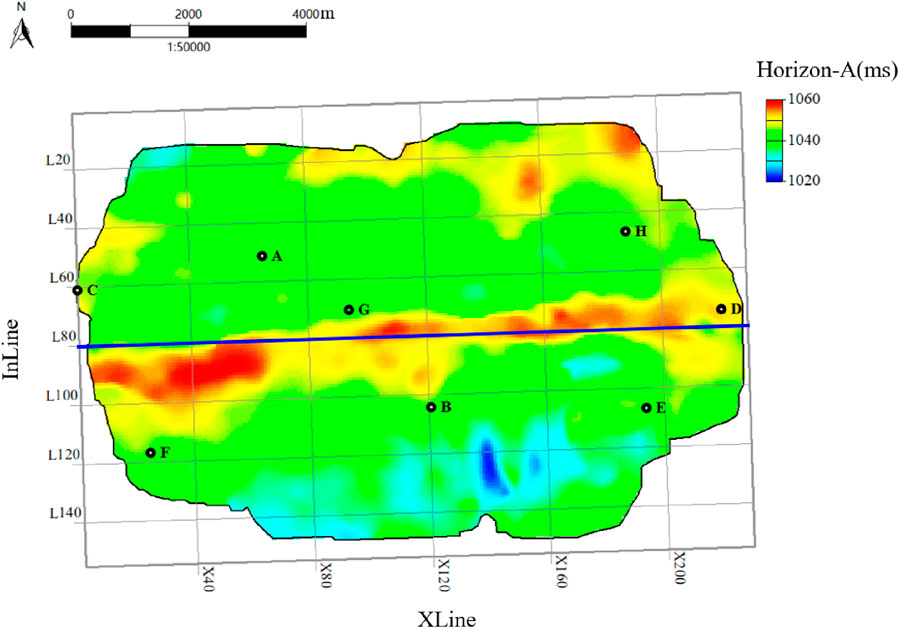
Figure 5. Map of the actual study area and well locations.

Figure 6

Figure 6. Seismic profile of inline 80.

Figure 7

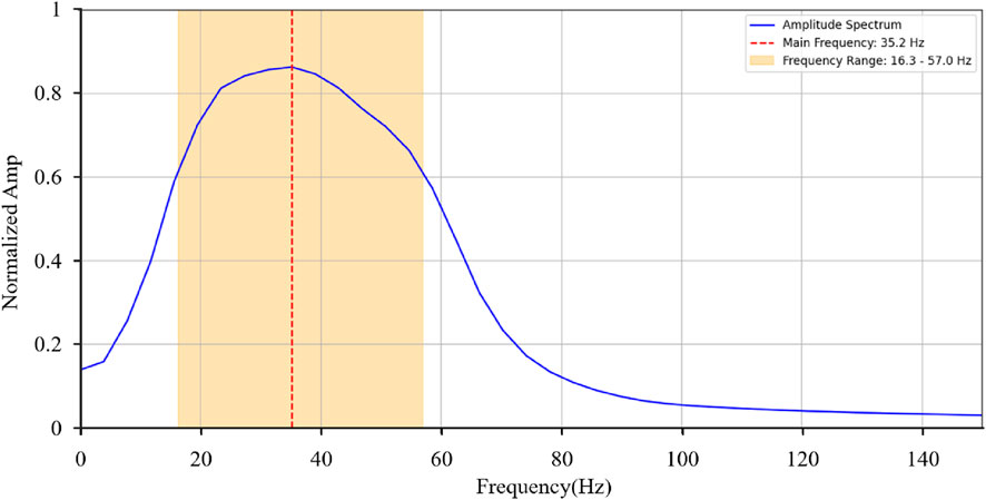
Figure 7. Spectrum analysis of the entire field data.

To clarify the overall workflow, Figure 8 presents a new flowchart summarizing the key steps of our proposed Cascaded Matching Optimization (CMO)-based automatic well-seismic tie method. This flowchart highlights the three main components of the process: data quality control, the core methodology including synthetic trace generation and cascaded optimization, and final validation through multi-well consistency checks, time-depth relationship analysis, and correlation coefficient evaluation. This structured workflow ensures that each phase of the process is both traceable and reproducible.

Figure 8

Figure 8. Workflow of automatic well-seismic calibration using CMO in the field data.

We take well-F as an example to illustrate the detailed steps of the automatic tie procedure. Well-F has undergone comprehensive preprocessing of the logging data. First, the reflection coefficients are calculated using the sonic logging data (Figure 9a) and density logging data (Figure 9b) from Well F. Next, the initial time-depth relationship (Figure 9c) is determined from the sonic travel time logs. The reflection coefficients (Figure 9d) are then converted from depth to the time domain, and finally, they are convolved with a given 35 Hz ricker wavelet to generate the synthetic trace (Figure 9e). From the seismic profile crossing the well (Figure 9f), it can be observed that there is a certain discrepancy between seismic horizons A and B and the well log markers A and B. The factors contributing to this mistie are complex. One major factor is that the sonic log data is not measured from the surface. In areas without sonic log data, the average seismic velocity of the overlying strata is typically used to calculate time. As a result, the synthetic trace computed in this manner will exhibit an overall time shifts relative to the nearby seismic trace.

Figure 9

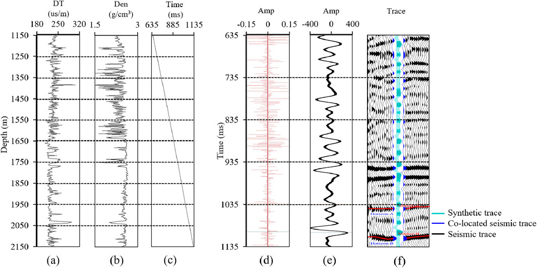
Figure 9. Synthetic trace generation and seismic well tie for well-F. (a) Acoustic log curve of well-F. (b) Density log curve of well-F. (c) Time-depth relationship calculated from the acoustic log. (d) Reflectivity sequence calculated from the acoustic and density logs, converted to the time domain using the time-depth relationship. (e) Synthetic trace generated by convolving the reflectivity sequence with the wavelet. (f) Seismic profile through the well-F.

The input well-side seismic trace (blue curve in Figure 10a) and the synthetic trace (red curve in Figure 10a) are used to calculate their local similarity attribute, which is a two-dimensional matrix. This local similarity attribute is normalized, and the result is shown in Figure 10b. We pick the time shifts from the local similarity attribute (black curve in Figure 10b). These time shifts are then applied to correct the synthetic trace. As shown in Figure 10c, the seismic marker layers around 1,035 m and 1,100 m have been successfully aligned with the corresponding well-log stratification, indicating that the initial correction effectively captures the layer correspondence between the well and seismic data. Moreover, the synthetic trace does not exhibit excessive stretching or compression during this process, preserving its waveform characteristics. It is worth noting that the similarity measure used in LSS is based on amplitude energy correlation rather than signal polarity. As a result, even when the synthetic and seismic traces are nearly opposite in polarity (as observed at the beginning of the trace), the similarity can still be high. This explains the high similarity around zero shift in Figure 10b, despite the apparent sign reversal. To address this issue, we further applied DTW to compute the residual time shifts between the corrected synthetic trace and the seismic trace near the well. The cumulative error matrix for this computation is shown in Figure 10d. Using the path traceback algorithm, the time shifts are picked (black curve in Figure 10d) and reapplied to the synthetic trace (red curve in Figure 10c). As shown in Figure 10e, the synthetic trace corrected through this cascaded matching optimization demonstrates a significantly improved alignment with the seismic trace. This approach effectively eliminates the remaining time discrepancies while preserving the original waveform characteristics of the wavelet group.

Figure 10

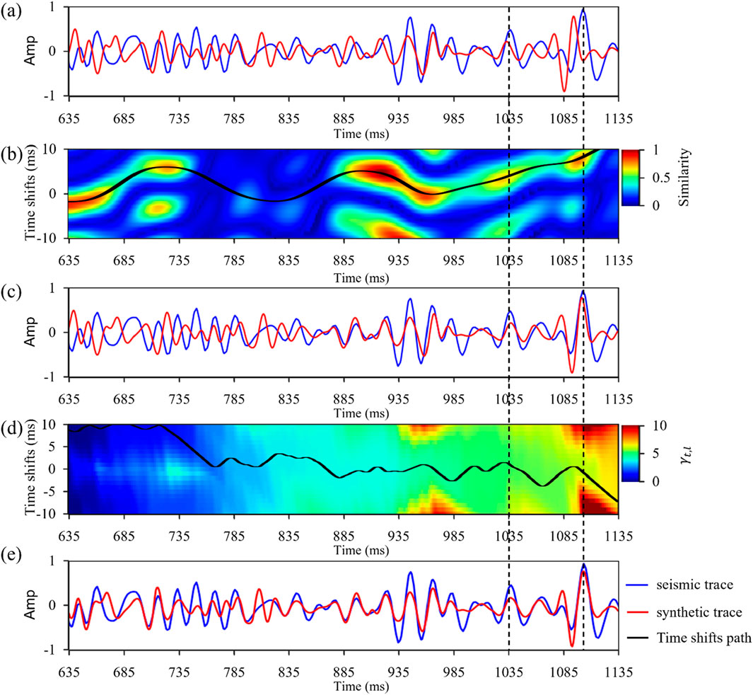
Figure 10. Automatic seismic-well tie of well-F using the cascaded matching optimization method. (a) Before the automatic well-seismic tie. (b) Local similarity matrix and time shifts. (c) Initial correction of the synthetic trace using LCC. (d) Cumulative error matrix calculated by comparing the initially corrected synthetic trace with the nearby well log. (e) Final automatic well-seismic tie result.

As shown in Figure 11, the synthetic traces before and after automated tie are compared along the well-crossing profile. By employing the cascaded matching optimization method, the calibrated synthetic trace exhibits excellent consistency with the seismic data in the well-crossing profile. Furthermore, an inspection of the sonic curves reveals no significant distortions or anomalies, indicating that the synthetic trace avoided excessive stretching and compression. This demonstrates this method’s effectiveness in achieving accurate and stable seismic well tie while preserving the original waveform characteristics.

Figure 11

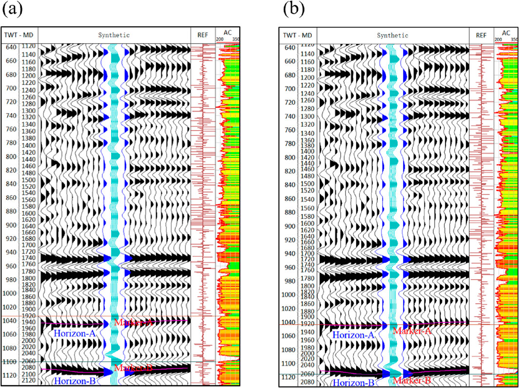
Figure 11. Well-F’s seismic profile through the well. (a) Before the automatic well-seismic tie. (b) After automatic well-seismic tie using cascaded matching optimization.

To further demonstrate the superiority of the proposed method, we conducted a comparative analysis with two commonly used automatic seismic-well tie methods: DTW and Windowed Time-Lag Cross-Correlation (WTLCC). Figure 12 illustrates the results for Well-F using different methods: the synthetic trace before calibration, the result calibrated with the cascaded matching optimization method, the result calibrated using DTW, and the result calibrated using WTLCC. Although the synthetic trace calibrated with DTW achieve the highest correlation coefficient with the seismic trace, this is achieved at the expense of excessively reducing cumulative errors, leading to pathological stretching and compression. For instance, at 800 m (highlighted by the green circle), two distinct peaks in the original synthetic trace are forcibly compressed into one, significantly distorting the original waveform characteristics. In contrast, the cascaded matching optimization method effectively preserves these features while achieving a high degree of tie accuracy. The WTLCC method shows suboptimal matching in multiple regions due to its limited ability to adapt to nonlinear time shifts, further emphasizing the robustness and adaptability of the proposed cascaded matching optimization approach.

Figure 12

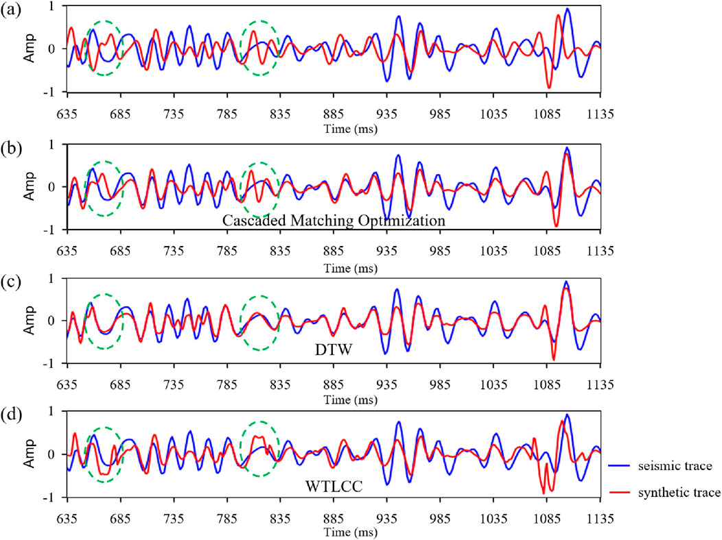
Figure 12. Comparison of automatic well-seismic tie results using different methods. (a) Before tie. (b) Automatic tie using cascaded matching optimization. (c) Automatic tie using DTW. (d) Automatic tie using WTLCC.

Using the cascaded matching optimization method, automatic seismic-well tie is performed for the remaining seven wells in the field data. In this region, the stratigraphy exhibits continuous lateral distribution, and the seismic response is characterized by continuous or sub-continuous reflectors. Synthetic traces generated from well logs along the seismic profile are expected to display similar waveform characteristics. By analyzing the cross-well profile, it is possible to evaluate whether changes in reflectors at well locations are geologically reasonable and whether geological boundaries align with seismic horizons. Figure 13 shows the cross-well profile from the study area. After applying the cascaded matching and optimization method, the synthetic traces at well locations exhibit strong vertical and lateral waveform consistency with the neighboring seismic traces, verifying the reliability of the automatic seismic-well tie results. Figure 14 shows the correlation coefficients of eight wells before and after CMO-based automatic well-seismic tie. The orange bars represent the correlation coefficients obtained using only a global bulk shift (Hall, 2012), while the blue bars indicate the results after applying the proposed method. A comparison clearly demonstrates a significant improvement in the correlation coefficients.

Figure 13

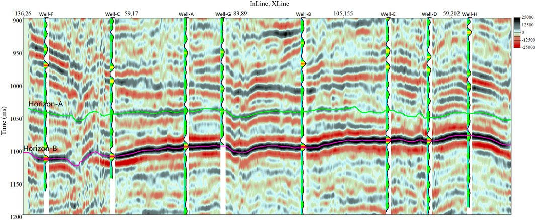
Figure 13. Well-to-well seismic profiles of eight wells after automatic tie using cascaded matching optimization.

Figure 14

Figure 14. Correlation coefficient plot between synthetic trace and near-well seismic trace.

Finally, multi-well time-depth relationship fitting is conducted as an additional quality control step for the eight wells. Within this study area, the time-depth relationships of multiple wells should exhibit a certain level of consistency. If the slope of a particular well deviates significantly—either too steep or too flat—it may indicate excessive stretching or compression during the calibration process. Conversely, if the slopes are consistent but the curves exhibit vertical shifts, it may suggest significant errors in calculating the initial start time of the synthetic traces. The multi-well time-depth relationships obtained after applying the cascaded matching optimization method are shown in Figure 15. These relationships are convergent and smooth, further demonstrating the overall high quality of the seismic-well tie calibration in the study area.

Figure 15

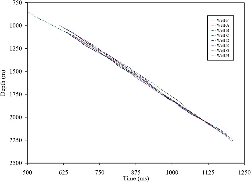
Figure 15. Time-depth relationship curves for eight wells after automatic tie using cascaded matching optimization.

4 Discussion

Seismic-well tie is a highly challenging task, as highlighted by the five steps outlined in the introduction. This study primarily focuses on the fifth step, but the preceding four steps inevitably influence its outcome to varying degrees. First, we recommend thoroughly inspecting sonic and density log data using borehole diameter logs to ensure no additional errors are introduced during the preprocessing stage. In the second step, because well-log data are recorded in the depth domain while seismic data are typically in the time domain, it is necessary to establish an initial time-depth relationship. Ideally, this would be done using checkshot surveys or Vertical Seismic Profiles (VSP) (Hornby et al., 2006), which provide direct measurements for accurate time-depth conversion. However, this study specifically addresses situations in which such datasets are unavailable. In such cases, we construct the time-depth relationship by integrating the velocity information from P-wave sonic logs. Traditionally, checkshot surveys provide discrete time-depth pairs. These are obtained by measuring the one-way travel time from the surface to downhole receivers and can be used to derive reliable average interval velocities. VSP data, in contrast, enable high-resolution imaging around the borehole and capture both upgoing and downgoing wavefields, improving interpretations of complex stratigraphy and reflector polarity. However, in many real-world exploration or development scenarios—especially in older wells or cost-constrained projects—checkshot and VSP data are often missing or incomplete. Our method addresses these challenges by leveraging P-wave sonic and bulk density logs to generate synthetic seismograms and build the initial time-depth relationship through velocity integration. This provides a practical and cost-effective alternative in data-limited environments. Nevertheless, a major limitation is the lack of calibration: without checkshot or VSP data to anchor the velocity field, the resulting time-depth relationship may deviate from the true seismic response. To mitigate this issue in practice, we recommend matching prominent reflectors in seismic data with key stratigraphic markers interpreted from well logs to reduce alignment errors and enhance tie accuracy. Overall, although our approach cannot fully replace the precision enabled by checkshot or VSP data, it offers broader applicability and greater flexibility in scenarios where such data are not available. It therefore expands the feasibility of seismic-well tie in data-constrained environments, enabling effective integration of well and seismic information with minimal additional cost.

During the wavelet estimation, multiple parameter adjustments should be conducted to select an appropriate wavelet, as this significantly influences the creation of synthetic traces and thereby affects the accuracy and reliability of automatic seismic-well tie. In this study, we utilized a constant-phase wavelet determined through phase rotation and peak amplitude analysis (van der Baan, 2008). Although using time-variant wavelets for calibration (Cai et al., 2023) could enhance accuracy, the increased complexity may pose challenges. This will be a focus of future research to further refine the proposed method. Additionally, it is crucial to ensure polarity consistency between seismic data and well logs (Gratwick and Finn, 2005), as incorrect polarity could result in automatic tie failure. High signal-to-noise ratio seismic data are also indispensable for successful seismic-well tie. Careful consideration of velocity modeling, particularly ensuring consistency between well and seismic velocities (Bader et al., 2018; Wo et al., 2024) is essential for improving the correlation between synthetic seismograms and seismic traces near the wellbore.

The focus of this study is on the fifth step of the well-seismic tie process, namely the alignment of synthetic seismograms with seismic traces in the vicinity of wells. Before the development of automatic or semi-automatic techniques, this task was typically performed manually by interpreters. While manual well tying benefits from the interpreter’s geological understanding and experience, it suffers from limited repeatability and poor scalability. This challenge becomes particularly significant in high-density well networks, such as those in certain oilfields in eastern China. For example, in the Shengli Oilfield, the well density can reach up to 275 wells per square kilometer, making manual well-seismic tie an extremely time-consuming process. DTW aims to find a locally optimal path by matching points one-to-one. In contrast, LSS allows for cross-sequence jumps, which are locally suboptimal. As a result, DTW tends to introduce more local stretching and squeezing. Although such adjustments can increase the correlation coefficient, as shown in Figure 3c, they often lead to distorted waveforms and potentially pathological matches. The LSS method, by enabling cross-sequence alignment, is better suited for preserving waveform characteristics during the initial matching stage, thereby providing a more reliable starting point for subsequent DTW application. Consequently, a cascaded matching optimization strategy is considered meaningful and beneficial. However, interpreters are advised to evaluate the final automated tying results using the quality control procedures proposed in this study. The quality of a well-seismic tie should not be judged solely by correlation coefficients (Herrera and van der Baan, 2014). A more comprehensive evaluation involves examining the calibrated acoustic logs. As illustrated in Figure 11, the AC logs before and after calibration show no distortion, only a minor overall shift. Moreover, the synthetic seismograms display minimal waveform variation, and the alignment between seismic events and geological layering is satisfactory. For multi-well scenarios, a post-calibration time-depth crossplot can be generated. In a localized survey area, the time-depth relationships among different wells are expected to be relatively consistent. Significant deviations in slope for individual wells may suggest over-stretching or compression during calibration. If the slopes are similar but exhibit vertical offsets, the starting time of the synthetic seismogram may have been incorrectly calculated. Lastly, inter-well section analysis provides additional validation. Within a stratigraphically continuous block, reflectors are expected to display consistent or quasi-consistent seismic phases. Synthetic traces constructed from logs along such sections should present comparable waveform features. This allows for evaluation of the consistency of reflection events at well locations and the match between geological stratigraphy and seismic horizons, further supporting the reliability of the well tie.

5 Conclusion

LSS and DTW each have inherent limitations in automated seismic-well tie. LSS excels in calculating time shifts while preserving waveform features but often leaves residual time shifts uncorrected. Conversely, DTW eliminates time discrepancies as much as possible but fails to maintain waveform coherence. The cascaded matching optimization method integrates the strengths of both approaches. It first employs LSS to compute smooth time shifts and then applies DTW under these constraints to calculate residual time shifts. This combined approach achieves improved matching by correcting time shifts while preserving waveform characteristics. This method offers a practical solution for achieving high-precision seismic-well ties, demonstrating significant potential for improving the accuracy and efficiency of well-seismic integration in reservoir characterization and seismic interpretation.

Data availability statement

The original contributions presented in the study are included in the article/supplementary material, further inquiries can be directed to the corresponding authors.

Author contributions

ML: Conceptualization, Validation, Writing – original draft, Writing – review and editing. XH: Funding acquisition, Supervision, Visualization, Writing – review and editing. WC: Investigation, Methodology, Writing – original draft, Writing – review and editing. YW: Methodology, Validation, Visualization, Writing – review and editing. MX: Data curation, Project administration, Resources, Writing – review and editing. MR: Conceptualization, Software, Supervision, Writing – review and editing. SL: Formal Analysis, Methodology, Validation, Writing – original draft.

Funding

The author(s) declare that financial support was received for the research and/or publication of this article. This study was funded by the National Natural Science Foundation of China (Grant No. 42241206 and No. 42174180).

Conflict of interest

Author MX was employed by Chuanqing Drilling Engineering Company. Author WC was employed by Schlumberger.

The remaining authors declare that the research was conducted in the absence of any commercial or financial relationships that could be construed as a potential conflict of interest.

Generative AI statement

The author(s) declare that no Generative AI was used in the creation of this manuscript.

Publisher’s note

All claims expressed in this article are solely those of the authors and do not necessarily represent those of their affiliated organizations, or those of the publisher, the editors and the reviewers. Any product that may be evaluated in this article, or claim that may be made by its manufacturer, is not guaranteed or endorsed by the publisher.

References

Anderson, P., and Newrick, R. (2008). Strange but true stories of synthetic seismograms. CSEG Rec. 12 (1), 51–56. doi:10.1190/segam2018-2998324

CrossRef Full Text | Google Scholar

Bader, S., Fomel, S., and Xue, Z. (2018). “Using well-seismic mistie to update the velocity model,” in SEG technical program expanded abstracts 2018, 5218–5222.

Google Scholar

Cai, S., Fang, F., and Wang, Y. (2023). Nonstationary seismic–well tying with time-varying wavelets. Geophysics 88, M145–M155. doi:10.1190/geo2022-0217.1

CrossRef Full Text | Google Scholar

Cui, T. (2015). Improving seismic-to-well ties. Canada: University of Calgary.

Google Scholar

Di, H., and Abubakar, A. (2023). Automating seismic-well tie via self-supervised learning. Geophys. Prospect. 71, 698–712. doi:10.1111/1365-2478.13333

CrossRef Full Text | Google Scholar

Duchesne, M. J., and Gaillot, P. (2011). Did you smooth your well logs the right way for seismic interpretation? J. Geophys. Eng. 8, 514–523. doi:10.1088/1742-2132/8/4/004

CrossRef Full Text | Google Scholar

El Dally, N. H., Metwalli, F. I., and Ismail, A. (2023). Seismic modelling of the upper cretaceous, khalda oil field, shushan basin, western desert, Egypt. Model. Earth Syst. Environ. 9, 4117–4134. doi:10.1007/s40808-022-01497-1

CrossRef Full Text | Google Scholar

Fomel, S. (2007a). Local seismic attributes. Geophysics 72, A29–A33. doi:10.1190/1.2437573

CrossRef Full Text | Google Scholar

Fomel, S. (2007b). Shaping regularization in geophysical-estimation problems. GEOPHYSICS 72, R29–R36. doi:10.1190/1.2433716

CrossRef Full Text | Google Scholar

Fomel, S. (2009). Velocity analysis using AB semblance. Geophys. Prospect. 57, 311–321. doi:10.1111/j.1365-2478.2008.00741.x

CrossRef Full Text | Google Scholar

Fomel, S., and Jin, L. (2009). Time-lapse image registration using the local similarity attribute. GEOPHYSICS 74, A7–A11. doi:10.1190/1.3054136

CrossRef Full Text | Google Scholar

Gratwick, D., and Finn, C. (2005). What's important in making far-stack well-to-seismic ties in West Africa? Lead. Edge 24, 739–745. doi:10.1190/1.1993270

CrossRef Full Text | Google Scholar

Hale, D. (2006). “Fast local cross-correlations of images,” in SEG International Exposition and Annual Meeting, New Orleans, Louisiana, October 1–6, 2006, 3160–3164.

Google Scholar

Hale, D. (2009). A method for estimating apparent displacement vectors from time-lapse seismic images. Geophysics 74, 2939–2943. doi:10.1190/1.2793081

CrossRef Full Text | Google Scholar

Hale, D. (2013). Dynamic warping of seismic images. Geophysics 78, S105–S115. doi:10.1190/geo2012-0327.1

CrossRef Full Text | Google Scholar

Hall, M. (2012). 52 things you should know about geophysics. Agile Libre.

Google Scholar

Herrera, R. H., Fomel, S., and van der Baan, M. (2014). Automatic approaches for seismic to well tying. Interpretation 2, SD9–SD17. doi:10.1190/INT-2013-0130.1

CrossRef Full Text | Google Scholar

Herrera, R. H., and van der Baan, M. (2012). “Guided seismic-to-well tying based on dynamic time warping,” in SEG International Exposition and Annual Meeting, Las Vegas, Nevada, November 4–9, 2012, 1–5.

Google Scholar

Herrera, R. H., and van der Baan, M. (2014). A semiautomatic method to tie well logs to seismic data. Geophysics 79, V47–V54. doi:10.1190/geo2013-0248.1

CrossRef Full Text | Google Scholar

Hornby, B. E., Yu, J., Sharp, J. A., Ray, A., Quist, Y., and Regone, C. (2006). VSP: beyond time-to-depth. Lead. Edge 25, 446–452. doi:10.1190/1.2193224

CrossRef Full Text | Google Scholar

Martinson, D. G., and Hopper, J. R. (1992). Nonlinear seismic trace interpolation. Geophysics 57, 136–145. doi:10.1190/1.1443177

CrossRef Full Text | Google Scholar

Martinson, D. G., Menke, W., and Stoffa, P. (1982). An inverse approach to signal correlation. J. Geophys. Res. Solid Earth 87, 4807–4818. doi:10.1029/JB087iB06p04807

CrossRef Full Text | Google Scholar

Metwalli, F. I., Ismail, A., and Pigott, J. D. (2024). “Advances in seismic and well log in the exploration in north africa,” in The geology of north africa. Editors Z. Hamimi, M. C. Chabou, E. Errami, A-R. Fowler, N. Fello, and A. Masrouhi (Cham: Springer International Publishing), 557–589.

CrossRef Full Text | Google Scholar

Munoz, A., and Hale, D. (2012). Automatically tying well logs to seismic data. CWP-725.

Google Scholar

Santos, L. S. O., Lemos, J. B., Souza, P, and Cerqueira, A. G. (2024). Automatic zero-phase wavelet estimation from seismic trace using a multilayer perceptron neural network: an application in a seismic well-tie. J. Appl. Geophys. 222, 105305. doi:10.1016/j.jappgeo.2024.105305

CrossRef Full Text | Google Scholar

van der Baan, M. (2008). Time-varying wavelet estimation and deconvolution by kurtosis maximization. Geophysics 73, V11–V18. doi:10.1190/1.2831936

CrossRef Full Text | Google Scholar

White, R., and Simm, R. (2003). Tutorial: good practice in well ties. First break 21, 75–83. doi:10.3997/1365-2397.21.10.25640

CrossRef Full Text | Google Scholar

Wo, Y., Zhou, H., Huang, X., Yue, Y., and Zou, Z. (2024). First-arrival traveltime tomography with near-surface structural regularization. IEEE Trans. Geosci. Remote Sens. 62, 1–14. doi:10.1109/TGRS.2024.3434396

CrossRef Full Text | Google Scholar

Wo, Y., Zong, J., Zhou, H.-W., Li, K., Yue, Y., and Huang, X. (2025). Near-surface structural regularization for full-waveform inversion using directional total variation. IEEE Trans. Geosci. Remote Sens. 63, 1–12. doi:10.1109/TGRS.2025.3541802

CrossRef Full Text | Google Scholar

Wu, H., Li, Z., Liu, N., and Zhang, B. (2022). Improved seismic well tie by integrating variable-size window resampling with well-tie net. J. Pet. Sci. Eng. 208, 109368. doi:10.1016/j.petrol.2021.109368

CrossRef Full Text | Google Scholar