Enhancing seabed sediment classification with multibeam echo-sounding and self-training: a case study from the East Sea of South Korea

Introduction: Accurate classification of seabed sediments is essential for marine spatial planning, resource management, and scientific research. While direct sampling yields precise sediment information, it is costly and spatially limited. Multibeam echo-sounding systems (MBES) offer broad coverage but lack detailed sediment characterization, creating a need for an integrated, data-driven approach.

Methods: We developed a machine-learning framework that fuses MBES backscatter data with limited seabed samples. Missing MBES values were first interpolated using a U-Net model to create a complete raster dataset. Advanced texture and spectral descriptors—Gray-Level Co-occurrence Matrix, Law’s texture filters, and discrete wavelet transforms—were extracted from the backscatter imagery. Five classifiers (Random Forest, Support Vector Machine, Deep Neural Network, Extreme Gradient Boosting, Light Gradient-Boosting Machine) were trained to predict four sediment classes (gravel, sand, clay, silt). To mitigate sample scarcity and class imbalance, a semi-supervised self-training loop iteratively added high-confidence pseudo-labels to the training set.

Results: Field validation in the East Sea (Republic of Korea) showed that the Extreme Gradient Boosting model achieved the highest accuracy. Overall prediction accuracy increased from 60.81 % with the baseline workflow to 72.73 % after applying data interpolation, enhanced feature extraction, and self-training.

Discussion: The proposed combination of U-Net interpolation, multi-scale texture features, and semi-supervised learning significantly improves sediment classification where MBES data are incomplete and sediment samples are sparse. This integrated workflow demonstrates the potential of machine-learning techniques to advance seabed mapping and support informed marine resource management.

1 Introduction

Seabed sediments play a crucial geological role, functioning as archives of Earth’s environmental history by preserving detailed records of climate change, oceanographic processes, and ecosystem dynamics over geological timescales (McNeill et al., 2019; Harris and Baker, 2011; Baker et al., 2021). Understanding the spatial distribution and composition of seabed sediments has emerged as a fundamental requirement for addressing multiple contemporary challenges in marine science and management (Zeppilli et al., 2016). These sediments not only influence benthic biodiversity patterns and ecosystem functioning but also provide essential baseline information for sustainable marine resource exploitation, environmental impact assessment, and climate change research (Kaikkonen et al., 2021).

Direct sediment sampling, a fundamental technique in seabed sediment research, involves the collection of sediment samples using box corers and grab samplers (Herkül et al., 2017). This method enables precise analysis of the physical and chemical properties of seabed sediments, accurately identifying components, particle sizes, and organic content (He et al., 2020). Direct sampling provides unparalleled ground-truth data, allowing detailed determination of grain size distribution, mineralogical composition, organic matter content, and contamination levels (Mudroch and Azcue, 1995). However, sampling is limited by high operational costs, low spatial coverage, logistical constraints in deep-sea surveys, vessel time availability, and dependency on weather conditions (Brown et al., 2011).

In contrast, acoustic remote sensing using multibeam echo-sounding (MBES) offers complementary capabilities that can address many of these limitations. MBES systems provide continuous, high-resolution bathymetric and backscatter intensity data over extensive seafloor areas (Ferrini and Flood, 2006). Backscatter intensity reflects the seafloor’s acoustic characteristics, influenced by factors such as sediment type, grain size, roughness, and physical properties (density, sound speed, attenuation) (Brown and Blondel, 2009; Gaida et al., 2019). This method efficiently captures geomorphological features, textural variations, and broad-scale sediment distribution patterns at a lower per-unit cost compared to direct sampling.

However, acoustic methods alone often provide insufficient detail for accurate sediment classification due to ambiguities caused by environmental factors and the indirect nature of acoustic signatures (Brown et al., 2012). Consequently, accurate seabed sediment mapping typically requires integrating acoustic data with ground-truth sediment sampling (Misiuk et al., 2018).

Traditional seabed sediment classification methods using MBES data heavily rely on expert interpretation and manual analysis (Dupre et al., 2014). This approach, while valuable, faces scalability limitations and subjective biases. Recent developments in machine learning and deep learning techniques have shown promising results in automating seabed sediment classification by learning nonlinear relationships between acoustic data and sediment properties (Diesing et al., 2016; Garone et al., 2023). Machine learning approaches are effective at extracting complex patterns from large datasets, providing consistency and efficiency, and overcoming limitations of manual interpretation and classical geostatistical methods (Berthold et al., 2017; Hasan et al., 2012; Lucieer et al., 2013).

Despite these advancements, significant challenges remain due to inherent data acquisition constraints. Specifically, there is a notable imbalance between the large volumes of multibeam data collected and the relatively sparse sediment samples available for training (Hu et al., 2023). This imbalance can cause model overfitting and degrade prediction accuracy (Ying, 2019). Therefore, there is an urgent need for advanced analytical approaches that can effectively utilize limited ground-truth data in combination with extensive but indirect acoustic data.

To address these fundamental challenges, we introduce an integrated workflow combining data interpolation, advanced feature extraction, and semi-supervised self-training. A U-Net convolutional neural network is employed to interpolate missing MBES data, preserving fine-scale seabed features better than conventional methods. Feature extraction methods, including Gray-Level Co-occurrence Matrix (GLCM), Law’s Texture, and discrete wavelet transform (DWT), are utilized to derive texture and terrain characteristics from acoustic data, enriching the predictive feature space.

Semi-supervised self-training, an iterative approach using pseudo-labeled data, is then applied to mitigate class imbalance and leverage the vast unlabeled acoustic dataset, improving the predictive performance of sediment classification models (Wei et al., 2021). This approach allows models to learn progressively from limited labeled samples and extensive unlabeled data, enhancing their robustness and generalization capability.

This study focuses on the East Sea continental shelf and slope, specifically the Ulleung Basin off South Korea, where we have 95 m-resolution MBES data paired with a limited set of 553 sediment samples. To systematically evaluate the effectiveness of our proposed workflow, we address four primary research questions:

RQ1 – Predictive capacity under data limitations: Can we achieve practical accuracy in predicting sediment proportions (gravel, sand, silt, clay) given sparse sampling and medium-resolution acoustic data?

RQ2 – Performance of U-Net–based gap filling: To what extent does a U-Net interpolator outperform conventional linear and cubic interpolation methods in reconstructing missing acoustic data?

RQ3 – Benefit of texture/terrain features and self-training: How much improvement in overall accuracy and class-specific accuracy do advanced feature extraction and semi-supervised self-training provide relative to fully supervised baselines?

RQ4 – Spatial robustness and transferability: Does our integrated workflow consistently perform across different physiographic sub-regions (inner shelf, continental slope, outer shelf), and can it potentially be transferred to continental shelves outside the East Sea?

By addressing these questions, we aim to establish a robust, replicable framework capable of overcoming data acquisition challenges common to many marine settings. Our results provide practical insights for enhancing operational seabed sediment mapping practices, contributing to broader efforts in marine spatial planning, resource management, environmental monitoring, and sustainable governance of marine ecosystems.

In this study, we introduce a workflow that includes data interpolation, feature extraction, and self-training as shown in Figure 1. First, we use a U-Net model to interpolate missing values in the acquired multibeam data, resulting in complete datasets. Next, we perform feature extraction on the multibeam data, and the extracted features are used to train five machine learning models to classify seabed sediments. Using the generated features and multibeam data as inputs, along with sampling data as labels, the model conducts regression to predict the proportions of gravel, sand, clay, and silt in the seabed. The self-training process iterates based on the regression results, progressively enhancing the model’s predictive performance. Finally, the model’s predictions of seabed sediments are validated against actual field data obtained from the East Sea of South Korea, demonstrating improved accuracy and reliability.

Figure 1

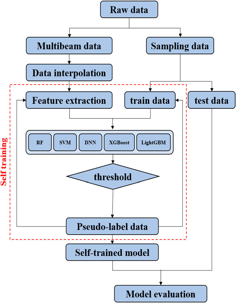
Figure 1. Workflow for seabed sediment classification using self-training approach.

2 Survey area and data

The survey area is in the East Sea of South Korea, covering the latitude range of 35.01–36.19 and the longitude range of 128.57–129.57 (Figure 2). This area can be divided into two regions. The inner continental shelf and the continental slope are mainly composed of fine sediment particles influenced by sea level changes, whereas the outer continental shelf consists of coarse residual sediment particles reflecting past environmental changes. Recent sediments from high sea level periods are predominantly found on the inner continental shelf, while residual sediments from low sea level periods are mainly distributed on the outer continental shelf. The continental slope is covered with fine sediments supplied by hemipelagic drift processes (Koo et al., 2014). The research area spans a range of 5,403 square kilometers, within which multibeam survey techniques were employed to acquire bathymetric and backscatter intensity data. Data acquisition took place between 2005 and 2021, and was conducted by the Korea Hydrographic and Oceanographic (KHOA). The data were carried out using the EM2040 multibeam echosounder and collected using HYPACK HYSWEEP, Qinsy, and Teledyne PDS as the primary acquisition platforms. The original multibeam data were acquired at a higher resolution, however, due to security restrictions imposed by the KHOA, only a 95 m resolution version of the data was made available for use in this study. The resolution of the multibeam data is crucial for covering large survey areas efficiently while still capturing fine-scale seabed features. The bathymetry (bathy) data shows that the depth of the study area ranges from 3 to 163 m, and the backscatter (bs) intensity ranges from −68.4 to 3.4 dB. Within the survey area, a total of 229,301 data points were acquired for both the ‘bathy’ and ‘bs’ variables. Sampling data was collected from a total of 553 locations in the survey area using grab and box corers. The sampling data includes location information, inclusion ratios of gravel, sand, silt, and clay, and sediment type. The pixel size of the multibeam data is (1,369, 440), and the sampling data has been randomly split into train and test data at a ratio of 8:2 for sediment classification.

Figure 2

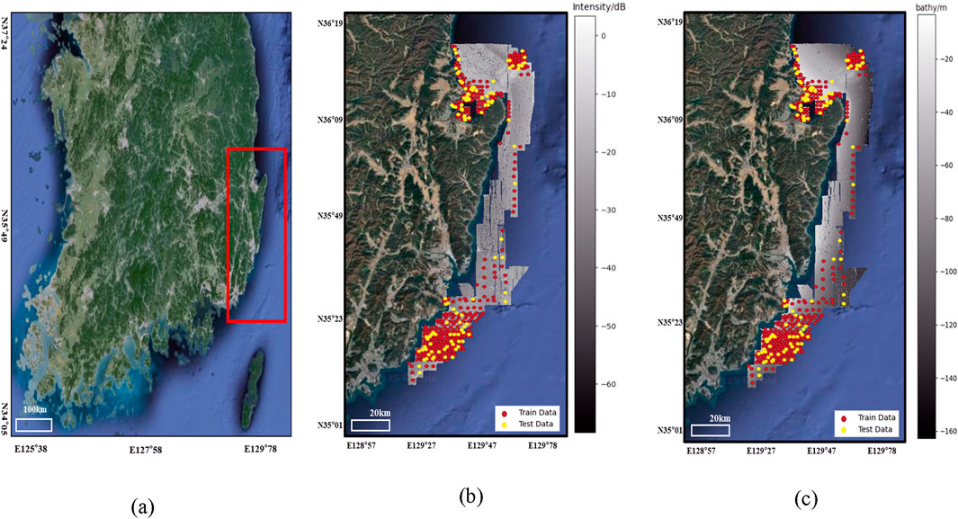
Figure 2. Map of South Korea, with the survey area highlighted in a red box (a). Multibeam backscatter data (b), bathymetry (c), and sampling points within the survey area in the East Sea of South Korea.

3 Data preprocessing

3.1 Headings interpolation of missing multibeam data using U-Net

Device limitations, economic constraints, and local maritime conflicts often result in significant gaps in MBES data, including bathymetry and backscatter data (Li et al., 2023). Similarly, in our study, missing data issues also occurred due to factors such as fishing activities, restricted access to shallow waters that are difficult for survey vessels to navigate, and unusable data that could not be processed properly. These missing values can increase uncertainty and introduce bias in seabed sediment predictions, ultimately reducing accuracy (Sánchez-Arcilla et al., 2021). To mitigate this issue, this study employs a deep learning-based interpolation technique using the U-Net model to fill these gaps and enhance data completeness and usability. The U-Net is a convolutional neural network (CNN) known for its symmetrical structure, which accurately separates and identifies fine details in images (Ronneberger et al., 2015). The model consists of two main parts: the encoder and the decoder. The encoder extracts important features from the input image, progressively reducing their size, while the decoder enlarges these features to restore detailed aspects of the image (Siddique et al., 2021). Skip connections directly connect features from each level of the encoder to the corresponding level of the decoder, minimizing information loss and enabling the decoder to accurately reproduce fine textures and details (Zhou et al., 2018).

In this study, we used a modified U-Net architecture to address the challenge of interpolating missing multibeam sonar data. As input, we use a randomly half-removed image from a 28 × 28 patch of multibeam data, and train an interpolation model by comparing it to the original patch. The model structure first applies a Random Masking layer to the input image to add random masking only during training. It then follows a typical U-Net structure, extracting features with two max poolings and concatenating them with the output of the previous layer in a subsequent upsampling step to restore detail. The end result is an output with two channels, which is an interpolated version of the original image. The analysis in this study was conducted using Python as the programming language. For machine learning and deep learning tasks, we utilized Scikit-learn and TensorFlow as the main frameworks. The network is trained using an Adam optimizer and a mean squared error loss function, with epoch set to 100. Early termination and model checkpoint callbacks are used to optimize the performance of the model. The interpolation process for this model can be seen in Figure 3.

Figure 3

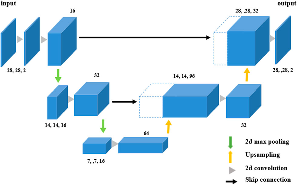
Figure 3. U-net architecture.

For training the interpolation model, the multibeam data is split into training, validation, and test datasets as shown in Figure 4a. Patches of 28 × 28 pixels without missing values were extracted, resulting in 133,537 training patches, 889 validation patches, and 119 testing patches. During training, 50% of the pixels in each patch were randomly removed to serve as input, while the complete patches were used as labels (Figure 4b). This approach enables the U-Net model to learn meaningful patterns from incomplete data and effectively fill the missing values, thereby enhancing its interpolation performance in real-world environments. After training the interpolation models, the performance of the interpolation results was compared with outcomes obtained using linear and cubic interpolation methods on the test dataset (Figures 4c–e).

Figure 4

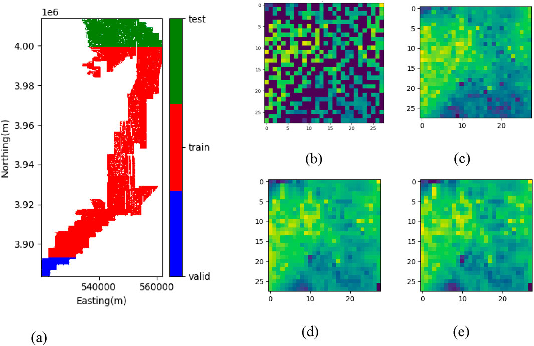
Figure 4. Data split for MBES data interpolation and examples of interpolation methods: (a) Division of survey area into training, validation, and testing area, (b) input patch with missing values, interpolation results of (c) U-Net, (d) Linear interpolation, and (e) Cubic interpolation.

The evaluation metrics employed were the Root Mean Square Error (RMSE) and the Peak Signal-to-Noise Ratio (PSNR) as follows:

$\text{RMSE}=\sqrt{\frac{1}{n}{{\displaystyle \sum _{i=1}^n}\left(Y_i-{\widehat{Y}}_i\right)}^2}(1)$

$PSNR=20·{\log }_{10}\left(\frac{{\mathit{MAX}}_I}{\sqrt{MSE}}\right)(2)$

In Equation 1, n is the number of patches, $Y_i$ is the complete patch from bathymetry or backscatter data, $\widehat{Y_i}$ is the predicted data, and in Equation 2, ${\mathit{MAX}}_I$ is the maximum possible value in the data. RMSE measures the discrepancy between actual and predicted values, where a lower value indicates greater similarity (Chai and Draxler, 2014). PSNR quantitatively assesses the quality difference between the original and processed images, with a higher value indicating a closer resemblance to the original image (Hore and Ziou, 2010).

The comparison showed that the U-Net model achieved the highest performance with an RMSE of 0.8825 and a PSNR of 49.4400 across both metrics, indicating an improvement over linear and cubic models (Table 1). Finally, the U-Net models for bathymetry and backscatter data are applied to the original multibeam data. After performing the interpolation, the missing values were effectively corrected, demonstrating the efficacy of the U-Net models in enhancing data completeness (Figure 5). One can also notice that the interpolation model extrapolates the data.

Table 1

Table 1. Performace comparisons for U-Net, Linear, and Cubic interpolations on the test dataset.

Figure 5

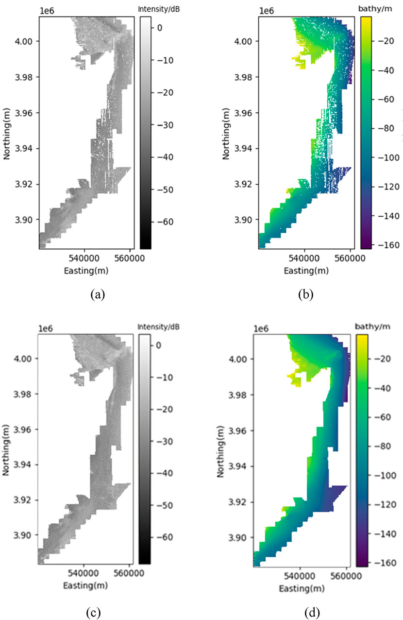
Figure 5. Before and after data interpolation using U-Net on backscatter and bathymetry data.(a) origin backscatter. (b) Origin bathymetry. (c) Interpolated backscatter. (d) Interpolated bathymetry.

3.2 Feature extraction

Feature extraction typically involves synthesizing information or attributes that describe the elements of an image to be classified in image classification (Ruiz et al., 2011). Through feature extraction, relevant shape information contained in patterns is described, allowing for the classification of patterns through a standardized procedure. This process enables the extraction of the most relevant information from the original data and its representation in a lower-dimensional space (Kumar and Bhatia, 2014). Feature extraction from multibeam backscatter data for seabed sediment classification plays a crucial role in the fields of marine science and resource management. Backscatter data obtained using multibeam acoustic technology reflects the surface characteristics of the seabed, and analyzing this data enables the identification of the seabed’s physical structure and sediment types (Preston, 2009).

Seabed roughness, which influences multibeam data, can be represented as texture characteristics, and in this paper, features were extracted using a texture matrix-based Gray-Level Co-occurrence Matrix (GLCM), Law’s texture, and wavelet decomposition based on discrete wavelet transform (DWT). GLCM is utilized to analyze the texture characteristics of sediments, extracting features that represent the surface texture and structure of the sediment to distinguish between various types of sediments (Pican et al., 1998). The GLCM calculation formula is based on the following research (Cinar et al., 2021). Law’s Texture is employed to analyze the texture energy patterns of seabed sediments, aiding in the identification of distinctive textures of the seabed topography by understanding the various characteristics of the sediments (Massot-Campos et al., 2013). This method utilizes convolutional kernels to extract texture features by emphasizing different spatial frequency components, enabling the differentiation of sediment types based on their textural properties (Haralick et al., 1973). DWT is used to decompose images or acoustic data of seabed sediments into different frequency components, facilitating the analysis of diverse topographical features and structures of the seabed through multiscale analysis (Cui et al., 2020)..

3.2.1 GLCM calculation

GLCM is a matrix-based computational method that yields features for gray-level space. In a GLCM matrix shown in Equation 3, $\mathrm{P}\left[\mathrm{i},\mathrm{j}\right]$ represents the frequency of occurrence of gray levels i and j for each pair of pixels in the image when the two pixels are at a certain distance and orientation.

$\mathrm{P}\left(\mathrm{i},\mathrm{j}\right)=\left[\begin{array}{cc}P\left(1,1\right)& P\left(1,N_g\right)\\ P\left(N_g,1\right)& P\left(N_g,N_g\right)\end{array}\right](3)$

3.2.2 Mean

The mean (Equation 4) represents the overall brightness level of the image. Areas with higher brightness are likely to have more fine-grained sediment, such as sand, while darker areas may have more coarse-grained sediment, such as gravel or bedrock (Samsudin and Hasan, 2017).

$\text{Mean}=\mathrm{\mu }=\frac{1}{n^2}{\displaystyle \sum _{i=0}^{n-1}}{\displaystyle \sum _{j=0}^{n-1}}i\times P\left[i,j\right](4)$

3.2.3 Variance

The variance in Equation 5 is calculated by averaging the squares of the observations minus the mean. Indicates texture variability in the image, with high variance indicating a mix of different grain sizes and compositions. High dispersion indicates an inhomogeneous surface with a mix of different grain sizes, most likely a sediment with a mixture of gravel and sand (Menandro et al., 2022).

$\text{Variance}=\mathrm{\sigma }=\frac{1}{n^2}{\displaystyle \sum _{i=0}^{n-1}}{\displaystyle \sum _{j=0}^{n-1}}{\left(i-\mathrm{\mu }\right)}^2\times P\left[i,j\right](5)$

3.2.4 Homogeneity

Indicates how uniformly distributed the sediment is. Higher values indicate a more uniform texture, with similar grain size and composition. A seafloor with high homogeneity is likely to be a homogeneous surface composed of fine-grained sediments (Sathiyamoorthi et al., 2021).

$Homogeneity=\frac{1}{n^2}{\displaystyle \sum _{i=0}^{n-1}}{\displaystyle \sum _{j=0}^{n-1}}\frac{P\left[i,j\right]}{1+{\left(i-j\right)}^2}(6)$

3.2.5 Contrast

Contrast represents the difference in brightness between pixels and helps you assess surface texture and grain size differences on the seafloor. Areas of high contrast can indicate uneven textures, such as clastic sediments or bedrock (Park, Y., and Guldmann, 2020).

$\text{Contrast}=\frac{1}{n^2}{\displaystyle \sum _{i=0}^{n-1}}{\displaystyle \sum _{j=0}^{n-1}}{\left(i-j\right)}^2\times P\left[i,j\right](7)$

3.2.6 Dissimilarity

Dissimilarity is calculated by summing the absolute value of the brightness differences between pixels, and high dissimilarity can indicate a large number of irregular sediments, such as assemblage sediments or cobbles, with large differences in grain size and composition (Alicia et al., 2023)

$\text{Dissimilarity}=\frac{1}{n^2}{\displaystyle \sum _{i=0}^{n-1}}{\displaystyle \sum _{j=0}^{n-1}}\left|i-j\right|\times P\left[i,j\right](8)$

3.2.7 Entropy

Entropy indicates the disorder and complexity of the seafloor, and a high entropy may suggest a seafloor with mixed sediments with complex and varying particle sizes, or a seafloor with many complex biological structures such as corals.

Entropy is a measure of the complexity of a texture distribution: a uniform distribution of values indicates low entropy, while large fluctuations indicate high entropy (Korda et al., 2022). So in an undersea environment, high entropy can indicate a seafloor with a complex mix of sediments of different particle sizes, or a seafloor with many complex biological structures such as coral.

$Entropy=-{\displaystyle \sum _{i=0}^{n-1}}{\displaystyle \sum _{j=0}^{n-1}}P\left[i,j\right]\times \mathit{log}\left(P\left[i,j\right]+ϵ\right)(9)$

3.2.8 Energy

Energy indicates the uniformity and repeatability of the texture, with surfaces with repetitive patterns having high energy values (Singh et al., 2017). High energy indicates fine-grained sediments with regular, repetitive patterns, often found in mud or uniform sandy sediments.

$Energy={\displaystyle \sum _{i=0}^{n-1}}{\displaystyle \sum _{j=0}^{n-1}}{\left(P\left[i,j\right]\right)}^2(10)$

3.2.9 Correlation

It represents the linear relationship between pixels and assesses the consistency of the pattern (Srivastava et al., 2020). If the correlation is high, the sediment is likely to have a regular, patterned structure. This can be seen in sediments with well-aligned grains.

$Correlation={\displaystyle \sum _{i=0}^{n-1}}{\displaystyle \sum _{j=0}^{n-1}}\frac{\left(i-{\mathrm{\mu }}_i\right)\times \left(j-{\mathrm{\mu }}_j\right)\times P\left[i,j\right]}{{\sigma }_i{\times \sigma }_j}(11)$

3.2.10 Auto-Correlation

Auto-Correlation indicates the degree of repetition of texture patterns and assesses the consistency of pixel (Soh and Tsatsoulis, 1999). High magnetic correlation can indicate fine-grained sediments, or seafloor surfaces with periodic patterns. For example, high magnetic correlation may be seen in structures such as regularly repeating sand patterns.

$Auto-Correlation={\displaystyle \sum _{i=0}^{n-1}}{\displaystyle \sum _{j=0}^{n-1}}i\times j\times P\left[i,j\right](12)$

Law’s texture is used to analyze texture energy patterns in seafloor sediments to help identify unique textures in seafloor topography by understanding the different characteristics of the sediments (Massot-Campos et al., 2013). Law’s texture consists of 1D vectors, each of size 5, that serve to emphasize each feature, and each of the vectors for level, edge, point, wave, and ripple are as follows L5 (level) = [1 4 6 4 1], E5 (Edge) = [-1 2 0 2 1], S5 (Spot) = [-1, 0, 2, 0, −1], W5 (wave) = [-1, 2, 0, −2, 1], R5 (ripple) = [1, −4, 6, −4, 1]. For each filter, a 2D convolutional mask is generated by combining the 1D vectors, and the features generated are L5E5, E5L5, E5S5, S5E5, S5R5, W5R5, R5W5, L5S5 and S5L5, for a total of 9 features.

DWT is used to decompose image or acoustic data of seafloor sediments into different frequency components to facilitate the analysis of different topography and structure of the seafloor through multiscale analysis (Cui et al., 2020). 2D Discrete Wavelet Transform (DWT) is a method to extract global and local texture information by separating low and high frequency components of seafloor sediment images. It is decomposed into four sub-bands: LL, LH, HL, and HH, where LL provides overall brightness and structure, LH and HL provide vertical and horizontal boundary information, and HH provides detailed texture. These texture features are used to distinguish grain size, pattern, and surface roughness of seafloor sediments, and can be fed into machine learning models to classify seafloor sediment types and generate distribution maps.

Bathymetric information significantly influences the distribution of seafloor sediments. Key geomorphometric variables derived from bathymetry include slope, aspect, roughness, and curvature (Janowski, 2025). Geologic texture features have a significant impact on seafloor bottom readings. These geometric features can provide reliable information by analyzing the underlying processes for seafloor structure. Based on this topographic information, you can ensure the accuracy and reliability of your terrain analysis for the predictions of your machine learning model (Janowski, 2025).

3.2.11 Slope

Slope measures the steepness of the seafloor, calculated as the rate of change in elevation over a certain distance. Steeper slopes are often associated with coarser sediments due to higher energy environments that prevent fine particles from settling, while flatter areas tend to accumulate finer sediments like silt and clay (Costello et al., 2010).

3.2.12 Aspect

Aspect refers to the compass direction that a slope faces, influencing sediment deposition patterns based on prevailing currents and wave action. For instance, slopes facing dominant currents may experience different sedimentation rates compared to those oriented away from such currents (Friedman et al., 2010).

3.2.13 Roughness

Roughness quantifies the variability in seafloor elevation, indicating the complexity of the terrain. Higher roughness values are linked to coarse materials like gravel or bedrock, while lower values correspond to finer sediments such as sand or mud (Volp et al., 2013).

3.2.14 Curvature

Curvature describes the concavity or convexity of the seafloor terrain. Positive curvature denotes convex features, and negative curvature indicates concave areas, aiding in predicting sediment erosion and deposition patterns.

These geomorphometric variables are crucial for understanding seafloor characteristics and have been effectively utilized in seabed mapping studies.

4 Modeling approach

4.1 Regression model

While our ultimate goal is to classify sediment types in the survey area, we begin by performing regression to predict the proportions of four sediment types: gravel, sand, clay, and silt. Based on these predicted proportions, we then classify the sediments by selecting the predominant type for each location. By shifting from categorical classification to quantitative regression models, this research aims to provide more accurate and practical insights into seabed composition (Stephens and Diesing, 2015). The regression models used in this study include Random Forest (RF), Support Vector Machine (SVM), Extreme Gradient Boosting (XGBoost), Light Gradient-Boosting Machine (LightGBM), and Deep Neural Network (DNN).

The Random Forest (RF) classifier is an ensemble classifier that generates multiple decision trees using a randomly selected subset of training samples and variables. The RF classifier effectively handles high data dimensionality and multicollinearity by aggregating the outputs of multiple decision trees, reducing variance and improving predictive performance. Additionally, it is relatively insensitive to overfitting because of its bootstrapped sampling approach and feature randomness (Breiman, 2001). However, it can be sensitive to the sampling design, meaning that biased or unrepresentative samples may impact classification accuracy (Belgiu and Drăguţ, 2016).

Support Vector Machine (SVM) is a machine learning model that classifies data by finding a decision boundary with maximum margin, mapping data points to a high-dimensional space. SVM uses key data points known as support vectors to define the decision boundary, aiding the model in effectively learning and generalizing complex data structures (Awad and Khanna, 2015).

Extreme Gradient Boosting (XGBoost) is an ensemble learning method combining decision trees, where each tree sequentially corrects the errors of its predecessor. This model maximizes computational efficiency through parallel processing, caching, and pruning techniques. Moreover, by handling missing data and optimizing various loss functions, it enhances the model’s accuracy and performance, demonstrating excellent capabilities in machine learning problems such as classification and regression (Chen and Guestrin, 2016).

Light Gradient Boosting Machine (LightGBM) is a high-performance gradient boosting framework that provides the capability to efficiently handle large datasets. This algorithm employs a boosting method that combines multiple weak prediction models to create a strong predictive model, using decision trees as its primary components. LightGBM constructs histograms of data, transforming continuous numerical data into discrete intervals, thus reducing memory usage and enhancing computational speed. One of the main advantages of this framework is its use of histogram-based algorithms to divide data into bins, which minimizes memory consumption and increases processing speed (Ke et al., 2017).

Deep neural network (DNN) is an Artificial Neural Network (ANN) structure composed of an input layer, an output layer, and multiple hidden layers in between. DNNs are structured to extract and learn complex features through several layers, allowing them to progressively recognize features from low-level to high-level abstract characteristics in input images (Sze et al., 2017).

In this study, Python was used as the primary programming language. For machine learning, we employed Scikit-learn, XGBoost, and LightGBM, while Tensorflow was utilized for deep learning applications. For the RF, SVM, XGBoost, and LightGBM models, optimal hyperparameters were determined using GridSearchCV. For the DNN, the model architecture includes layers with 64, 128, 256, 128, and 64 neurons each, utilizing ReLU as the activation function. The final layer features 4 neurons with softmax activation to ensure that the total proportions sum to one. The Adam optimizer is used to solve the optimization problem, using mean squared error (MSE) as the loss function.

4.2 Self-training

In the field of seabed classification, integrating multibeam and sampling data is crucial, yet the scarcity of sampling data remains a persistent issue. Acquiring sampling data is difficult and costly, and analyzing the acquired material requires significant time and resources. To address this challenge, this paper introduces a new approach using self-training based on semi-supervised learning to mitigate the problem of sparse sampling data. This method leverages the predictive power of labeled data while incorporating unlabeled data to enhance model performance, particularly in scenarios with limited ground-truth samples (Diesing et al., 2016). This method can play a crucial role in maximizing data utilization and enhancing the accuracy of seabed mapping (Amini et al., 2025).

The self-training approach begins with a small set of labeled data to train a base model. The model then predicts labels for the remaining unlabeled data, applying pseudo-labeling based on high-confidence predictions (Zoph et al., 2020). These pseudo-labeled samples are subsequently added to the training dataset as new labeled data for retraining. This iterative process, which is vital for maintaining the consistency and preventing bias across model predictions, continues until the model’s performance improves (Figure 6) (Chen et al., 2022; Scikit-learn developers, 2023).

Figure 6

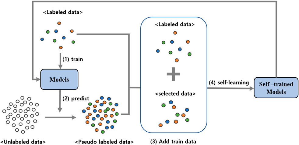
Figure 6. Illustration of the self-training process for model improvement.

The core of this methodology is that the model learns from its own predictions, using these insights to process unlabeled data and enrich the training set. This is especially beneficial in contexts where labeling large datasets is impractical or expensive (Kim and Shin, 2013). By expanding the training set through self-training, the model develops a deeper understanding of complex patterns, thereby improving its predictive accuracy and reliability in seabed classification.

In this paper, we perform self-training in the following steps. First, we train five regression models (RF, DNN, SVM, LightGBM, and XGBoost) with the initial training material. The five trained models make predictions on the unlabeled data. The prediction is performed by a regression process that finds the ratio values of the four classes: gravel, sand, silt, and clay. The predicted results of the five models are averaged and this average value is pseudo-labeled. Compare the MSE values of the results predicted by the five models based on the pseudo-labeled values, and select the 10 samples with the smallest average MSE for each class for the pseudo-labeled unlabeled data and add them to the original train data. The remaining unlabeled data except the added data is initialized and used for prediction again in the next step. 1 cycle is done through the process described above and repeated until the number of data in each class is twice as large as the class with the most data. The self-training was repeated for a total of 44 cycles. In this way, the original 553 data were increased to 258 data for each of the four classes, totaling 1,032 data. These self-trained data are then used to train the seafloor sediment prediction model.

5 Results

The model’s performance was assessed using five regression models on the test dataset across four distinct classes, which varied in the use of feature extraction and self-training. Specifically, we categorized the regression results into four types—gravel, sand, silt, and clay—based on the highest proportion of these types present, and calculated the overall accuracy and class-specific accuracy for the test dataset.

As illustrated in Table 2, the base models without feature extraction or self-training exhibited poor performance, with accuracies ranging from 44.74% to 60.81%. However, the introduction of feature extraction and self-learning significantly enhanced performance. Notably, XGBoost demonstrated the most substantial improvement, with accuracy increasing from 56.75% to 72.73%. Table 3 presents the confusion matrix for the test dataset using XGBoost with feature extraction and self-training. In detail, the model showed good performance in predicting sand and silt, achieving Producer’s Accuracies (PA) of over 75%. However, there are still significant challenges in accurately predicting gravel and clay. The poor gravel prediction is attributed to its minimal presence in the training set, leading to inadequate learning and higher misclassification rates. The low accuracy in predicting clay can be attributed to the inherent difficulty in distinguishing between silt and clay, as these sediment types have very similar physical and acoustic properties. Nevertheless, this rise in accuracy across scenarios indicates that both the feature extractions and the integration of self-training are crucial in enhancing model performance on the test dataset.

Table 2

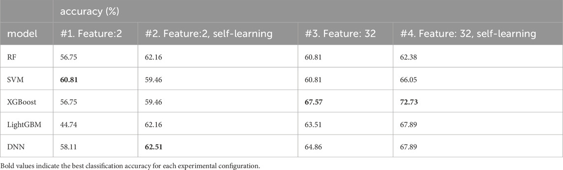
Table 2. Performance of five models under conditions of feature extraction and Self-training.

Table 3

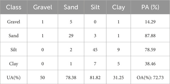
Table 3. Confusion matrix for the XGBoost model with feature extraction and self-training on the test dataset.

Further analysis involved using the XGBoost models to classify the entire survey area under four scenarios of feature extraction and self-training, as shown in Figure 7. For result verification, we compared our models’ predictions with the sediment type distribution data of the East Sea provided by Korea GeoBigData (Figure 7a) (Park, 2016). This region is predominantly composed of M, (g)M, sM, gsM, mS, and (g)mS sediment classes. Each class consists of the following approximate proportions: M (Mud): Nearly 100% mud (silt + clay), with no significant sand or gravel. (g)M (Slightly Gravelly Mud): Composed of ∼95% mud with a small amount of gravel (∼0–5%). sM (Sandy Mud): Contains ∼60–80% mud and ∼20–40% sand, with no gravel. gsM (Gravelly Sandy Mud): Made up of ∼60–70% mud, ∼20–30% sand, and ∼5–10% gravel. mS (Muddy Sand): Primarily ∼60–80% sand, with ∼20–40% mud. (g)mS (Slightly Gravelly Muddy Sand): Contains ∼50–70% sand, ∼20–40% mud, and ∼0–5% gravel. These sediment classifications reflect the varying depositional environments in the region, influenced by hydrodynamic conditions.

Figure 7

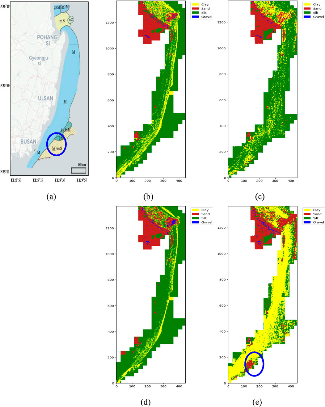
Figure 7. Seabed sediment type distribution results of the East Sea (a) and predicted distribution and seabed sediment mapping results in conditions (b): no feature extraction, no self-training, (c): feature extraction, no self-training, (d): no feature extraction, self-training, (e): feature extraction, self-training.

Predictions were consistently accurate across all scenarios, particularly in the mud belt area—a combination of silt and clay—in the middle part of the survey area. Enhanced predictions were noted under the scenario involving feature extraction and self-training, particularly in the northern mS region and the southern sM region. Additionally, the (g)mS region, highlighted by the blue circle in Figure 7a, which is partially included in our survey area, exhibited potential sand distribution, as indicated by the blue circle in Figure 7e, confirming that the scenario with the most advanced feature extraction and self-training yielded the best prediction results.

6 Discussion

6.1 Scientific and practical contributions

This study demonstrates significant advances in seabed sediment classification under realistic constraints, achieving an overall accuracy (OA) of 72.73% using only 553 sediment samples and relatively low-resolution (95 m) MBES data. Previous studies in seabed classification typically relied on extensive sampling and high-resolution acoustic datasets. However, this research proves that combining advanced feature extraction and semi-supervised self-training can yield practical accuracy comparable to fully supervised approaches despite severe data limitations. Specifically, the high producer’s accuracies achieved for sand (87.9%) and silt (78.6%) underline the potential of this workflow for reliably mapping sediment distributions at a regional scale, even when field sampling is sparse and acoustic data resolution is suboptimal.

From a marine geological perspective, achieving these accuracy levels with constrained datasets has considerable practical implications. Operational sediment mapping often faces financial, logistical, and environmental limitations, making extensive sampling and high-resolution acoustic data collection difficult. Thus, this study provides a scientifically grounded and economically feasible alternative, effectively bridging the gap between ideal research conditions and practical operational requirements. The methodological framework outlined here can be particularly valuable in preliminary assessments for marine spatial planning, habitat management, offshore infrastructure development, and environmental monitoring, where obtaining comprehensive field datasets is challenging.

6.2 Limitations

Despite these significant improvements, several inherent limitations remain and should be explicitly acknowledged. One critical issue is the mismatch in spatial resolution and temporal alignment between the MBES data and sediment samples. Each 95 m × 95 m MBES pixel integrates extensive spatial variability, whereas individual grab/core samples represent discrete, point-specific measurements. This mismatch likely introduces substantial uncertainty, potentially causing misclassifications by inadequately capturing the sediment heterogeneity within each pixel. Additionally, temporal discrepancies—up to 19 years between acoustic data collection and sediment sampling—further complicate classification accuracy, given that seabed sediment distributions can naturally vary over such timescales due to oceanographic and geomorphologic processes.

Another limitation is related to severe class imbalance in the training dataset. In particular, gravel samples were extremely scarce (only a single representative), significantly reducing model performance and reliability for this sediment type. The clay class similarly posed challenges due to its acoustic and textural similarity to silt, resulting in frequent confusion. These class imbalance issues reflect practical limitations in sample acquisition, affecting the robustness and generalization capabilities of the developed model. Statistical measures and field-based validation both indicate that resolving these class-specific challenges requires targeted sampling strategies or advanced data augmentation methods to ensure balanced representation across sediment types.

6.3 Future work and algorithmic improvements

The promising results of this study open several pathways for methodological expansion and practical application. First, extending the proposed approach through transfer learning to different marine regions represents a critical step in validating its generalization potential. Given variations in acoustic signatures, sediment properties, and oceanographic conditions across continental shelves, future studies should explicitly assess model transferability using domain adaptation techniques. These approaches would help refine the framework’s robustness, enabling broader applicability across diverse marine environments.

Also, algorithmic enhancements focusing on spatially explicit models—such as convolutional neural networks (CNNs)—are recommended to explicitly account for spatial correlation and feature neighborhood contexts inherent to seabed sediments. Additionally, adopting self-supervised learning (SSL) methods such as contrastive learning or masked autoencoders can extract robust features from extensive unlabeled acoustic datasets, improving downstream performance even with limited labeled samples (Caron et al., 2021). Incorporating uncertainty estimation methods, like Monte Carlo dropout or deep ensembles, will further enhance the practical utility of sediment predictions by quantifying confidence levels for decision-making in marine spatial planning contexts.

Collectively, these future directions not only promise improved classification accuracy but also provide novel insights into underlying marine geological processes, potentially enabling proactive detection of environmental change indicators through advanced machine learning techniques.

7 Conclusion

This study addressed the fundamental challenge of accurately mapping seabed sediments using limited ground-truth samples (553 points) and medium-resolution (95 m) MBES backscatter data. Our results demonstrate that integrating U-Net–based gap filling, advanced texture and terrain feature extraction, and semi-supervised self-training can achieve robust sediment classification accuracy of 72.7%, overcoming typical limitations associated with sparse sampling and coarse acoustic resolution.

The developed workflow notably improves sediment mapping accuracy (producer’s accuracies reaching 88% for sand and 79% for silt), showing that sophisticated machine-learning techniques effectively compensate for data scarcity, thus enabling reliable sediment mapping even in logistically constrained environments.

We propose that this modular and adaptable approach be further applied and fine-tuned across other continental shelves globally, with significant potential implications for marine spatial planning, environmental management, habitat conservation, offshore engineering, and sustainable marine resource assessment.

Data availability statement

The datasets presented in this article are not readily available because, due to security restrictions of the Korea Hydrographic and Oceannographic (KHOA), the authors do not have permission to share the original data.

Author contributions

CL: Methodology, Software, Writing – original draft. SP: Methodology, Software, Writing – original draft. DY: Conceptualization, Funding acquisition, Supervision, Writing – review and editing. B-YY: Data curation, Funding acquisition, Project administration, Writing – review and editing. ML: Data curation, Funding acquisition, Writing – review and editing.

Funding

The author(s) declare that financial support was received for the research and/or publication of this article. This research was supported by the Korea Institute of Marine Science & Technology Promotion (KIMST) funded by the Ministry of Oceans and Fisheries in 2023 (Development of technology for seabed classification based on machine learning, Management No. 20220254).

Acknowledgments

This research was supported by the Korea Institute of Marine Science & Technology Promotion (KIMST) funded by the Ministry of Oceans and Fisheries in 2023 (Development of technology for seabed classification based on machine learning, Management No. 20220254).

Conflict of interest

Author ML was employed by Marine Research Corporation.

The remaining authors declare that the research was conducted in the absence of any commercial or financial relationships that could be construed as a potential conflict of interest.

Generative AI statement

The author(s) declare that Generative AI was used in the creation of this manuscript. The author(s) verify and take full responsibility for the use of generative AI in the preparation of this manuscript. Generative AI was used.

Publisher’s note

All claims expressed in this article are solely those of the authors and do not necessarily represent those of their affiliated organizations, or those of the publisher, the editors and the reviewers. Any product that may be evaluated in this article, or claim that may be made by its manufacturer, is not guaranteed or endorsed by the publisher.

References

Alicia, R. R., Laura, M. L. H., Piotr, K., Maciej, C., and Piotr, B. (2023). Image analysis and benthic ecology: proceedings to analyze in situ long-term image series. Limnol. Oceanogr. Methods 21 (4), 169–177. doi:10.1002/lom3.10537

CrossRef Full Text | Google Scholar

Amini, M. R., Feofanov, V., Pauletto, L., Hadjadj, L., Devijver, E., and Maximov, Y. (2025). Self-training: a survey. Neurocomputing 616, 128904. doi:10.1016/j.neucom.2024.128904

CrossRef Full Text | Google Scholar

Awad, M., and Khanna, R. (2015). “Support vector machines for classification,” in Efficient learning machines: theories, concepts, and applications for engineers and system designers, 39–66. doi:10.1007/978-1-4302-5990-9_3

CrossRef Full Text | Google Scholar

Baker, B. J., Appler, K. E., and Gong, X. (2021). New microbial biodiversity in marine sediments. Annu. Rev. Mar. Sci. 13 (1), 161–175. doi:10.1146/annurev-marine-032020-014552

PubMed Abstract | CrossRef Full Text | Google Scholar

Belgiu, M., and Drăguţ, L. (2016). Random forest in remote sensing: a review of applications and future directions. ISPRS J. Photogrammetry Remote Sens. 114, 24–31. doi:10.1016/j.isprsjprs.2016.01.011

CrossRef Full Text | Google Scholar

Berthold, T., Leichter, A., Rosenhahn, B., Berkhahn, V., and Valerius, J. (2017). “Seabed sediment classification of side-scan sonar data using convolutional neural networks,” in 2017 IEEE symposium series on computational intelligence (SSCI), 1–8. doi:10.1109/SSCI.2017.8285220

CrossRef Full Text | Google Scholar

Breiman, L. (2001). Random forests. Mach. Learn. 45, 5–32. doi:10.1023/A:1010933404324

CrossRef Full Text | Google Scholar

Brown, C. J., and Blondel, P. (2009). Developments in the application of multibeam sonar backscatter for seafloor habitat mapping. Appl. Acoust. 70 (10), 1242–1247. doi:10.1016/j.apacoust.2008.08.004

CrossRef Full Text | Google Scholar

Brown, C. J., Sameoto, J. A., and Smith, S. J. (2012). Multiple methods, maps, and management applications: purpose made seafloor maps in support of ocean management. J. Sea Res. 72, 1–13. doi:10.1016/j.seares.2012.04.009

CrossRef Full Text | Google Scholar

Brown, C. J., Smith, S. J., Lawton, P., and Anderson, J. T. (2011). Benthic habitat mapping: a review of progress towards improved understanding of the spatial ecology of the seafloor using acoustic techniques. Estuar. Coast. Shelf Sci. 92 (3), 502–520. doi:10.1016/j.ecss.2011.02.007

CrossRef Full Text | Google Scholar

Caron, M., Touvron, H., Misra, I., Jégou, H., Mairal, J., Bojanowski, P., et al. (2021). “Emerging properties in self-supervised vision transformers,” in Proceedings of the IEEE/CVF International Conference on Computer Vision, Montreal, QC, Canada, 10-17 October 2021 (IEEE), 9650–9660.

CrossRef Full Text | Google Scholar

Chai, T., and Draxler, R. R. (2014). Root mean square error (RMSE) or mean absolute error (MAE)? Arguments against avoiding RMSE in the literature. Geosci. Model Dev. 7 (3), 1247–1250. doi:10.5194/gmd-7-1247-2014

CrossRef Full Text | Google Scholar

Chen, B., Jiang, J., Wang, X., Wan, P., Wang, J., and Long, M. (2022). Debiased self-training for semi-supervised learning. Adv. Neural Inf. Process. Syst. 35, 32424–32437. doi:10.5555/3600270.3602619

CrossRef Full Text | Google Scholar

Chen, T., and Guestrin, C. (2016). Xgboost: a scalable tree boosting system. Proc. 22nd ACM SIGKDD Int. Conf. Knowl. Discov. Data Min., 785–794. doi:10.1145/2939672.2939785

CrossRef Full Text | Google Scholar

Cinar, A., Topuz, B., and Ergin, S. (2021). A new region-of-interest (ROI) detection method using the chan-vese algorithm for lung nodule classification. Int. Adv. Res. Eng. J. 5 (2), 281–291. doi:10.35860/iarej.857579

CrossRef Full Text | Google Scholar

Costello, M. J., Cheung, A., and De Hauwere, N. (2010). Surface area and the seabed area, volume, depth, slope, and topographic variation for the world’s seas, oceans, and countries. Environ. Sci. and Technol. 44 (23), 8821–8828. doi:10.1021/es1012752

PubMed Abstract | CrossRef Full Text | Google Scholar

Cui, X., Xing, Z., Yang, F., Fan, M., Ma, Y., and Sun, Y. (2020). A method for multibeam seafloor terrain classification based on self-adaptive geographic classification unit. Appl. Acoust. 157, 107029. doi:10.1016/j.apacoust.2019.107029

CrossRef Full Text | Google Scholar

Diesing, M., Mitchell, P., and Stephens, D. (2016). Image-based seabed classification: what can we learn from terrestrial remote sensing? ICES J. Mar. Sci. 73 (10), 2425–2441. doi:10.1093/icesjms/fsw118

CrossRef Full Text | Google Scholar

Dupre, S., Berger, L., Le Bouffant, N., Scalabrin, C., and Bourillet, J. F. (2014). Fluid emissions at the Aquitaine Shelf (Bay of Biscay, France): a biogenic origin or the expression of hydrocarbon leakage? Cont. shelf Res. 88, 24–33. doi:10.1016/j.csr.2014.07.004

CrossRef Full Text | Google Scholar

Ferrini, V. L., and Flood, R. D. (2006). The effects of fine-scale surface roughness and grain size on 300 kHz multibeam backscatter intensity in sandy marine sedimentary environments. Mar. Geol. 228 (1-4), 153–172. doi:10.1016/j.margeo.2005.11.010

CrossRef Full Text | Google Scholar

Friedman, A., Pizarro, O., and Williams, S. B. (2010). “Rugosity, slope and aspect from bathymetric stereo image reconstructions,” in In Oceans’10 IEEE Sydney (IEEE), 1–9. doi:10.1109/OCEANSSYD.2010.5604003

CrossRef Full Text | Google Scholar

Gaida, T. C., Mohammadloo, T. H., Snellen, M., and Simons, D. G. (2019). Mapping the seabed and shallow subsurface with multi-frequency multibeam echosounders. Remote Sens. 12 (1), 52. doi:10.3390/rs12010052

CrossRef Full Text | Google Scholar

Garone, R. V., Birkenes Lønmo, T. I., Schimel, A. C. G., Diesing, M., Thorsnes, T., and Løvstakken, L. (2023). Seabed classification of multibeam echosounder data into bedrock/non-bedrock using deep learning. Front. Earth Sci. 11, 1285368. doi:10.3389/feart.2023.1285368

CrossRef Full Text | Google Scholar

Haralick, R. M., Shanmugam, K., and Dinstein, I. H. (1973). Textural features for image classification. IEEE Trans. Syst. man, Cybern. (6), 610–621. doi:10.1109/TSMC.1973.4309314

CrossRef Full Text | Google Scholar

P. Harris, and E. Baker (2011). Seafloor geomorphology as benthic habitat: GeoHab atlas of seafloor geomorphic features and benthic habitats (Elsevier).

Google Scholar

Hasan, R. C., Ierodiaconou, D., and Monk, J. (2012). Evaluation of four supervised learning methods for benthic habitat mapping using backscatter from multi-beam sonar. Remote Sens. 4 (11), 3427–3443. doi:10.3390/rs4113427

CrossRef Full Text | Google Scholar

He, S., Peng, Y., Jin, Y., Wan, B., and Liu, G. (2020). Review and analysis of key techniques in marine sediment sampling. Chin. J. Mech. Eng. 33, 66–17. doi:10.1186/s10033-020-00480-0

CrossRef Full Text | Google Scholar

Herkül, K., Peterson, A., and Paekivi, S. (2017). Applying multibeam sonar and mathematical modeling for mapping seabed substrate and biota of offshore shallows. Estuar. Coast. Shelf Sci. 192, 57–71. doi:10.1016/j.ecss.2017.04.026

CrossRef Full Text | Google Scholar

Hore, A., and Ziou, D. (2010). “Image quality metrics: PSNR vs. SSIM,” in 2010 20th International Conference on Pattern Recognition, Istanbul, Turkey, 23-26 August 2010 (IEEE), 2366–2369. doi:10.1109/ICPR.2010.579

CrossRef Full Text | Google Scholar

Hu, H., Feng, C., Cui, X., Zhang, K., Bu, X., and Yang, F. (2023). A sample enhancement method based on simple linear iterative clustering superpixel segmentation applied to multibeam seabed classification. IEEE Trans. Geoscience Remote Sens. 61, 1–15. doi:10.1109/TGRS.2023.3247827

CrossRef Full Text | Google Scholar

Janowski, Ł. (2025). Advancing seabed bedform mapping in the kułnica deep: leveraging multibeam echosounders and machine learning for enhanced underwater landscape analysis. Remote Sens. 17 (3), 373. doi:10.3390/rs17030373

CrossRef Full Text | Google Scholar

Kaikkonen, L., Helle, I., Kostamo, K., Kuikka, S., Tornroos, A., Nygård, H., et al. (2021). Causal approach to determining the environmental risks of seabed mining. Environ. Sci. and Technol. 55 (13), 8502–8513. doi:10.1021/acs.est.1c01241

PubMed Abstract | CrossRef Full Text | Google Scholar

Ke, G., Meng, Q., Finley, T., Wang, T., Chen, W., Ma, W., et al. (2017). “Lightgbm: a highly efficient gradient boosting decision tree,” in Advances in neural information processing systems, 30.

Google Scholar

Kim, J., and Shin, H. (2013). Breast cancer survivability prediction using labeled, unlabeled, and pseudo-labeled patient data. J. Am. Med. Inf. Assoc. 20 (4), 613–618. doi:10.1136/amiajnl-2012-001570

PubMed Abstract | CrossRef Full Text | Google Scholar

Koo, B. Y., Kim, S. P., Lee, G. S., and Chung, G. S. (2014). Seafloor morphology and surface sediment distribution of the southwestern part of the Ulleung Basin, East Sea. , East Sea. J. Korean earth Sci. Soc. 35 (2), 131–146. doi:10.5467/JKESS.2014.35.2.131

CrossRef Full Text | Google Scholar

Korda, A. I., Andreou, C., Rogg, H. V., Avram, M., Ruef, A., Davatzikos, C., et al. (2022). Identification of texture MRI brain abnormalities on first-episode psychosis and clinical high-risk subjects using explainable artificial intelligence. Transl. Psychiatry 12 (1), 481. doi:10.1038/s41398-022-02242-z

PubMed Abstract | CrossRef Full Text | Google Scholar

Kumar, G., and Bhatia, P. K. (2014). “A detailed review of feature extraction in image processing systems,” in 2014 Fourth International Conference on Advanced Computing and Communication Technologies, Rohtak, India, 08-09 February 2014 (IEEE), 5–12. doi:10.1109/ACCT.2014.74

CrossRef Full Text | Google Scholar

Li, Z., Peng, Z., Zhang, Z., Chu, Y., Xu, C., Yao, S., et al. (2023). Exploring modern bathymetry: a comprehensive review of data acquisition devices, model accuracy, and interpolation techniques for enhanced underwater mapping. Front. Mar. Sci. 10, 1178845. doi:10.3389/fmars.2023.1178845

CrossRef Full Text | Google Scholar

Lucieer, V., Hill, N. A., Barrett, N. S., and Nichol, S. (2013). Do marine substrates ‘look’and ‘sound’the same? Supervised classification of multibeam acoustic data using autonomous underwater vehicle images. Estuar. Coast. Shelf Sci. 117, 94–106. doi:10.1016/j.ecss.2012.11.001

CrossRef Full Text | Google Scholar

Massot-Campos, M., Oliver-Codina, G., Ruano-Amengual, L., and Miró-Juliá, M. (2013). “Texture analysis of seabed images: quantifying the presence of posidonia oceanica at palma bay,” in 2013 MTS/IEEE OCEANS-Bergen (IEEE), 1–6. doi:10.1109/OCEANS-Bergen.2013.6607991

CrossRef Full Text | Google Scholar

McNeill, L. C., Shillington, D. J., Carter, G. D., Everest, J. D., Gawthorpe, R. L., Miller, C., et al. (2019). High-resolution record reveals climate-driven environmental and sedimentary changes in an active rift. Sci. Rep. 9 (1), 3116. doi:10.1038/s41598-019-40022-w

PubMed Abstract | CrossRef Full Text | Google Scholar

Menandro, P. S., Bastos, A. C., Misiuk, B., and Brown, C. J. (2022). Applying a multi-method framework to analyze the multispectral acoustic response of the seafloor. Front. Remote Sens. 3, 860282. doi:10.3389/frsen.2022.860282

CrossRef Full Text | Google Scholar

Misiuk, B., Lecours, V., and Bell, T. (2018). A multiscale approach to mapping seabed sediments. PLoS One 13 (2), e0193647. doi:10.1371/journal.pone.0193647

PubMed Abstract | CrossRef Full Text | Google Scholar

Mudroch, A., and Azcue, J. M. (1995). Manual of aquatic sediment sampling. Boca Raton, FL: Crc Press.

Google Scholar

Park, J. (2016). Marine geological and geophysical mapping of the Korean seas. Final Rep. Daejeon, Republic of Korea: Korea Institute of Geoscience and Mineral Resources; TRKO201700000450. doi:10.23000/TRKO201700000450

CrossRef Full Text | Google Scholar

Park, Y., and Guldmann, J. M. (2020). Measuring continuous landscape patterns with Gray-Level Co-Occurrence Matrix (GLCM) indices: an alternative to patch metrics? Ecol. Indic. 109, 105802. doi:10.1016/j.ecolind.2019.105802

CrossRef Full Text | Google Scholar

Pican, N., Trucco, E., Ross, M., Lane, D. M., Petillot, Y., and Ruiz, I. T. (1998). “Texture analysis for seabed classification: co-occurrence matrices vs. self-organizing maps,” in In IEEE Oceanic Engineering Society. OCEANS'98. Conference Proceedings (Cat. No. 98CH36259), Nice, France, 28 September 1998 - 01 (IEEE), 424–428. doi:10.1109/OCEANS.1998.725781

CrossRef Full Text | Google Scholar

Preston, J. (2009). Automated acoustic seabed classification of multibeam images of Stanton Banks. Appl. Acoust. 70 (10), 1277–1287. doi:10.1016/j.apacoust.2008.07.011

CrossRef Full Text | Google Scholar

Ronneberger, O., Fischer, P., and Brox, T. (2015). “U-net: convolutional networks for biomedical image segmentation,”, 18. Springer international publishing, 234–241. doi:10.1007/978-3-319-24574-4_28

CrossRef Full Text | Google Scholar

Ruiz, L. A., Recio, J. A., Fernández-Sarría, A., and Hermosilla, T. (2011). A feature extraction software tool for agricultural object-based image analysis. Comput. Electron. Agric. 76 (2), 284–296. doi:10.1016/j.compag.2011.02.007

CrossRef Full Text | Google Scholar

Samsudin, S. A., and Hasan, R. C. (2017). Assessment of multibeam backscatter texture analysis for seafloor sediment classification. Int. Archives Photogrammetry, Remote Sens. Spatial Inf. Sci. 42, 177–183. doi:10.5194/isprs-archives-XLII-4-W5-177-2017

CrossRef Full Text | Google Scholar

Sánchez-Arcilla, A., Gracia, V., Mösso, C., Cáceres, I., González-Marco, D., and Gómez, J. (2021). Coastal adaptation and uncertainties: the need of ethics for a shared coastal future. Front. Mar. Sci. 8, 717781. doi:10.3389/fmars.2021.717781

CrossRef Full Text | Google Scholar

Sathiyamoorthi, V., Ilavarasi, A. K., Murugeswari, K., Ahmed, S. T., Devi, B. A., and Kalipindi, M. (2021). A deep convolutional neural network based computer aided diagnosis system for the prediction of Alzheimer's disease in MRI images. Measurement 171, 108838. doi:10.1016/j.measurement.2020.108838

CrossRef Full Text | Google Scholar

Scikit-learn developers (2023). Semi-supervised learning. scikit-learn 1.4.1 documentation. Available online at: https://scikit-learn.org/stable/modules/semi_supervised.html.

Google Scholar

Siddique, N., Paheding, S., Elkin, C. P., and Devabhaktuni, V. (2021). U-net and its variants for medical image segmentation: a review of theory and applications. IEEE access 9, 82031–82057. doi:10.1109/ACCESS.2021.3086020

CrossRef Full Text | Google Scholar

Singh, S., Srivastava, D., and Agarwal, S. (2017). “GLCM and its application in pattern recognition,” in 2017 5th International Symposium on Computational and Business Intelligence (ISCBI), Dubai, United Arab Emirates, 11-14 August 2017 (IEEE), 20–25. doi:10.1109/ISCBI.2017.8053537

CrossRef Full Text | Google Scholar

Soh, L. K., and Tsatsoulis, C. (1999). Texture analysis of SAR sea ice imagery using gray level co-occurrence matrices. IEEE Trans. geoscience remote Sens. 37 (2), 780–795. doi:10.1109/36.752194

CrossRef Full Text | Google Scholar

Srivastava, D., Rajitha, B., Agarwal, S., and Singh, S. (2020). Pattern-based image retrieval using GLCM. Neural Comput. Appl. 32, 10819–10832. doi:10.1007/s00521-018-3611-1

CrossRef Full Text | Google Scholar

Stephens, D., and Diesing, M. (2015). Towards quantitative spatial models of seabed sediment composition. PLoS One 10 (11), e0142502. doi:10.1371/journal.pone.0142502

PubMed Abstract | CrossRef Full Text | Google Scholar

Sze, V., Chen, Y. H., Yang, T. J., and Emer, J. S. (2017). Efficient processing of deep neural networks: a tutorial and survey. Proc. IEEE 105 (12), 2295–2329. doi:10.1109/JPROC.2017.2761740

CrossRef Full Text | Google Scholar

Volp, N. D., Van Prooijen, B. C., and Stelling, G. S. (2013). A finite volume approach for shallow water flow accounting for high-resolution bathymetry and roughness data. Water Resour. Res. 49 (7), 4126–4135. doi:10.1002/wrcr.20324

CrossRef Full Text | Google Scholar

Wei, C., Sohn, K., Mellina, C., Yuille, A., and Yang, F. (2021). “Crest: a class-rebalancing self-training framework for imbalanced semi-supervised learning,” in In Proceedings of the IEEE/CVF conference on computer vision and pattern recognition, Nashville, TN, USA, 20-25 June 2021 (IEEE), 10857–10866.

CrossRef Full Text | Google Scholar

Ying, X. (2019). An overview of overfitting and its solutions. J. Phys. Conf. Ser. 1168, 022022. doi:10.1088/1742-6596/1168/2/022022

CrossRef Full Text | Google Scholar

Zeppilli, D., Pusceddu, A., Trincardi, F., and Danovaro, R. (2016). Seafloor heterogeneity influences the biodiversity–ecosystem functioning relationships in the deep sea. Sci. Rep. 6 (1), 26352. doi:10.1038/srep26352

PubMed Abstract | CrossRef Full Text | Google Scholar

Zhou, Z., Rahman Siddiquee, M. M., Tajbakhsh, N., and Liang, J. (2018). “Unet++: a nested u-net architecture for medical image segmentation,” in In Deep learning in medical image analysis and multimodal learning for clinical decision support: 4th international workshop, DLMIA 2018, and 8th international workshop, ML-CDS 2018, held in conjunction with MICCAI 2018, Granada, Spain, September 20, 2018, proceedings 4 (Springer International Publishing), 3–11. doi:10.1007/978-3-030-00889-5_1

CrossRef Full Text | Google Scholar

Zoph, B., Ghiasi, G., Lin, T. Y., Cui, Y., Liu, H., Cubuk, E. D., et al. (2020). Rethinking pre-training and self-training. Adv. neural Inf. Process. Syst. 33, 3833–3845. doi:10.5555/3495724.3496047

CrossRef Full Text | Google Scholar