Ice loss detection of glacierets in the Desert and Central Andes of Chile between 2018 and 2023

Worldwide, the shrinkage of small glaciers has occurred more rapidly in recent decades, and the Desert and Central Andes of Chile are no exception. Among these ice bodies are glacierets, defined as glaciers with a reduced surface area of less than 25 km². Their extensive and heterogeneous distribution along the Andes makes their analysis challenging, yet the limited number of studies documenting glacieret’s change presents an opportunity to deepen the understanding of their response to anthropogenic climate change. In this work, we seek to detect, at the end of the austral summer of 2023, the variation of visible ice surfaces of glacierets between the Arica y Parinacota Region and the Biobío Region. A combined remote sensing approach is applied to analyse their surface cover through the Normalised Difference Snow Index (NDSI) along with albedo and land surface temperature changes using satellite inputs from Landsat 8 and Sentinel-2 imagery. We validate our results through a visual inspection for all the small glacierets (area below 0.01 km²) using high-resolution optical imagery for the period 2018–2023. Lastly, we corroborate the observed trends with temperature and precipitation data from meteorological stations. Our results evidence a general reduction of the clean ice area of 16%, equivalent to a surface ice loss of −4.77 km² for the 2019–2023 period for all 1,856 glacierets within the study area. This trend is shared by the smallest glacierets with more than 50% having no visible surface ice by 2023–2024, such that 77 glacierets are declared “entirely vanished” and 244 glacierets “presumably vanished,” with an ice loss of up to 1.49 km². Additionally, we found that more than 34% of the glacierets analysed could be considered debris-covered, with most of them located below 5,000 m a.s.l. throughout the study area. The observed glacieret’s surface changes are supported by a precipitation reduction of up to 80% in mountainous areas when comparing the 2018–2023 period with previous decades (2000–2023). Our findings represent a valuable contribution to local and regional hydrological assessments, particularly for regions in the Desert and Central Andes of Chile already subjected to hydrological stress.

1 Introduction

Chile concentrates approximately 80% of the surface area of all Andean glaciers and is in seventh place worldwide. Along the Andes, Chile has a wide variety of glaciers in terms of size and morphology. Such glacier diversity poses significant challenges to assessing the impact of anthropogenic climate change along its different regions (Ayala et al., 2020). From the large, debris-free outlet glaciers of the Southern and Northern Patagonian icefields with sizes exceeding the hundreds of square kilometres, passing to the debris-covered valley and mountain glaciers around tens of square kilometres, to the small glacierets of less than 0.25 km². Anthropogenic climate change is affecting every corner of the world (Arias et al., 2021). Along the Southern Andes, there has been a combination of increasing air temperature and decreasing precipitation trends in recent decades (Falvey and Garreaud, 2009; Boisier et al., 2016; Masiokas et al., 2019), although the latter shows larger interannual and inter-decadal variability (Garreaud, 2009). Nevertheless, this combination has led to an increase in the 0°C isotherm and the regional equilibrium line altitude (Carrasco et al., 2008) and the general shrinkage of glaciers (Braun et al., 2019; Dussaillant et al., 2019) and a decrease in snow cover (Cordero et al., 2019).

Worldwide, the shrinkage of small glaciers, including glacierets, has occurred more rapidly in recent decades in comparison with the end of the 20th century (Parkes and Marzeion, 2018), to the point of being the class size (below 0.5 km²) with the highest shrinkage rate for the Swiss Alps (Fischer et al., 2014). At the same time, in the Pyrenees (Izagirre et al., 2024), and other low-latitude regions such as Venezuela, Mexico, Indonesia and Africa (Carvalho Resende et al., 2022), these shrinking glaciers are the last remaining ice bodies. Higher shrinkage rates of small glaciers have been attributed to their lower accumulation area ratio (Parkes and Marzeion, 2018) and the observed global temperature increase (Zemp et al., 2015). However, some of them, when constrained to the most elevated and sheltered areas, start to attenuate their response to climate change due to local topographic factors influencing their mass balance (Florentine et al., 2018), demonstrating that they are decoupled from regional climate forcing. This is the case for avalanche-fed and debris-covered small glaciers (Huss and Fischer, 2016).

Recently, the Chilean General Water Directorate (DGA) presented the latest version of the glaciers inventory in Chile, called the Public Glacier Inventory, hereby referred to as IPG2022. This is an excellent opportunity to study one of the most numerous but, at the same time, least studied ice masses, the glacierets. Cogley et al. (2011) define glacierets as small glaciers, typically less than 0.25 km² in extent, with no marked flow pattern visible at the surface and no distinct shape. To qualify as a glacieret, an ice body must persist for at least two consecutive years. However, according to the IPG2022 (DGA, 2022), this temporal condition is extended to five consecutive years. In addition, the IPG2022 considers that all ice masses, excluding rock glaciers, of less than 0.25 km², regarding shape and percentage of debris-covered surface, are classified as glacierets.

Because of small-scale processes and complex feedback between precipitation, temperature, and radiative forcings, assessing glacierets response to climate change at regional scale is challenging (Huss and Fischer, 2016). Furthermore, the significant number and diversity of glacierets, (18,213 glacierets accounted for in Chile according to the IPG2022), along with the different climate regions of the Chilean Andes (arid, semi-arid, mediterranean, temperate and cold-and-humid) makes it even more challenging to assess the sensitivity and response of these small ice masses to climate change.

Recent studies have provided relevant regional insights into glacier surface albedo changes for the central Chilean Andes from 1986 to 2020 (Shaw et al., 2021), geodetic mass balance patterns (elevation differences) for Andean glaciers from 2000 to 2018 (Dussaillant et al., 2019) and an overview of recent changes in Andean glaciers (Masiokas et al., 2020). However, the response of glacierets and small glaciers to climate change in South America is poorly documented. Studies include Ramírez et al. (2001) who document the volume changes of Chacaltaya Glacier in the Bolivian Andes between 1992 and 1998, prior to its complete vanishment by 2009 (Veettil and Kamp, 2019), the assessment of recent changes of small glaciers at the northeast margin of the Southern Patagonian Icefield from 1975 to 2005 by Masiokas et al. (2015) and the geodetic mass balance and area changes evaluation of Echaurren Norte Glacier in the Central Chilean Andes (Región Metropolitana in Figure 1), from 1955 to 2015, by Farías-Barahona et al. (2019). The latter being of particular importance since Echaurren Norte Glacier has the longest and continuous mass balance time series in South America since 1975 to the present (Masiokas et al., 2016; WGMS, 2021).

Figure 1

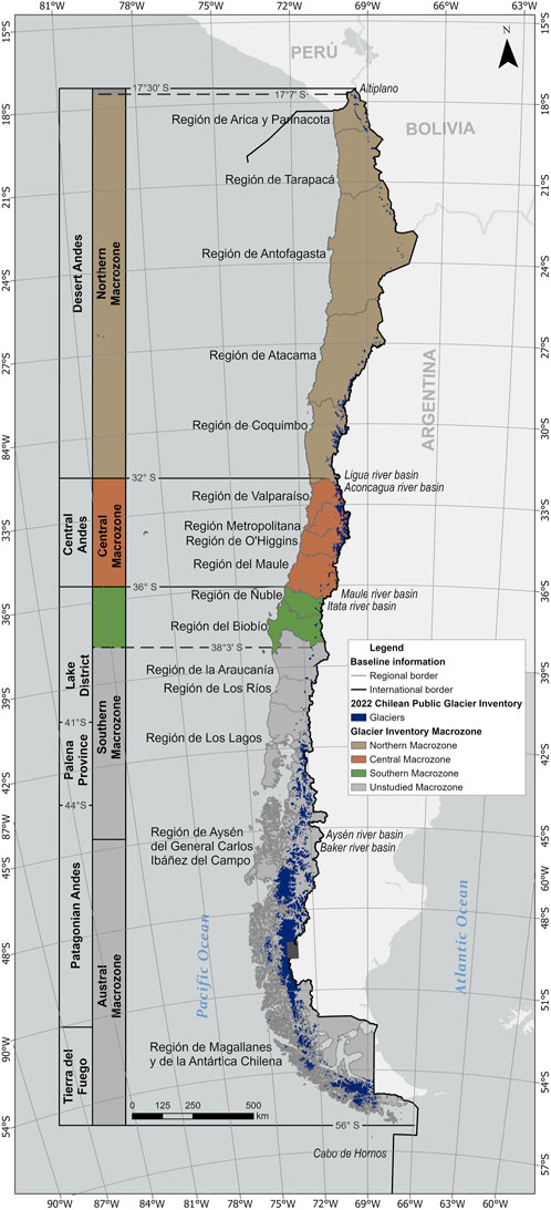
Figure 1. The Chilean Andes considered in this study (17.7°S −38.3°S). The three main glaciological macrozones assessed here are highlighted, as defined by the IPG2022, and their corresponding equivalence with Lliboutry’s glaciological zones (Desert, Central and, partially, the Lake District Andes) represented in the form of a latitudinal segmentation.

This study aims to fill this knowledge gap with a detailed assessment of recent changes of glacieret’s surface characteristics, such as the presence or absence of visible ice, existence of a debris cover, albedo and surface temperature, between the Arica y Parinacota Region and the Biobío Region, Desert and Central Andes of Chile (Northern, Central and Southern Glaciological Zones). Although the Ñuble and Biobío regions are part of the Southern Glaciological Zone according to the IPG2022, for this research, we include those regions indifferently as part of the Central Andes. Considering the latest version of the Chilean glacier inventory, IPG2022, we describe the morphological characteristics of Chile’s glacierets, then, we evaluate the recent changes of all the smallest glacierets (those with an extension less than 0.01 km²) included in the IPG2022 within our study area using high-resolution (submetric pixel size) remote sensing data, including the persistence, or absence, of visible surface ice. According to the IPG2022 mapping criteria, glaciers between 0.001 km² and 0.01 km² included in the current glacier inventory had to be mapped in the 2014 version of the IPG (Barcaza et al., 2017), thus, we test the hypothesis that these glacierets have lost ice throughout the 8 years between the glacier inventories (IPG2014 and IPG2022). To better assess recent surface changes (2020–2023) of all glacierets in the study area, we analyse albedo and surface temperature changes using remote sensing data (Sentinel-2 and Landsat 8 data) from the end of the 2020 and 2023 ablation seasons. Our analysis is followed by a meteorological characterisation based on local weather stations’ data.

We discuss our results regarding their statistical confidence, the glacieret’s surface characteristics and their recent changes throughout the 2018–2023 period. Our findings provide critical input to the glacieret’s response to anthropogenic climate change, such as albedo and land surface temperature variations, along with the potential vanishment of a significant portion of the analysed sample. In the context of the International Year of Glaciers’ Preservation, our study is a valuable contribution to local and regional hydrological assessments, particularly for regions in the Desert and Central Andes of Chile subjected to hydrological stress.

1.1 Study area

Chile extends along the Southern Andes over 4,000 km (17,5°–56° S). The vast latitude and elevation ranges create a large diversity of climates and, consequently, glaciers. Considering the difference in climate and elevation, Lliboutry (1998) divides the Southern Andes into four main zones: (i) Desert Andes, (ii) Central Andes, (iii) Lakes District Andes, and (iv) Patagonian Andes and Tierra del Fuego. Here we focus on the glacierets between the Arica y Parinacota Region and the Biobío Region (17.7°S–38.3°S). This latitudinal range spans throughout the Desert Andes, Central Andes, and part of the Lakes District glaciological zones, which are almost equivalent to the Northern, Central and, partially, the Southern glaciological zones of Chile (DGA, 2022; Barcaza et al., 2017) (Figure 1).

In total, 11 regions are considered in this study (Figure 1), with the Arica y Parinacota Region being the northernmost and Biobío Region the southernmost in the study area. According to the IPG2022, three out of four glaciological macrozones, or glaciological zones, are included in our study. The northern macrozone considers the regions of Arica y Parinacota, Tarapacá, Antofagasta, Atacama, and Coquimbo. Their climate is mainly characterised by hyper-aridity and semi-arid conditions (Aceituno, 1996). Most of the glaciers in this region are located at high elevations, either on the Altiplano or on mostly dormant volcanic ranges. In this macrozone, peaks with elevations over 5,000 m a.s.l. are common, a feature that decreases in number and elevation when moving southwards. The central macrozone includes the Valparaíso, Metropolitana, O’Higgins and Maule regions. Its climate is primarily Mediterranean with wet winters and dry summers (Garreaud et al., 2020). Elevations range from 4,000 to 5,000, with some scarce peaks over 6,000 m a.s.l., allowing the development of proper conditions for glaciers. Lastly, the Southern glaciological macrozone is partially covered, as this study only includes the Ñuble and Biobío regions. In contrast, the macrozone encompasses four additional regions to the south. In this zone, the elevation decreases drastically to 3,000 m a.s.l. on average, with some scarce peaks reaching elevations over 4,000 m a.s.l. Nonetheless, wetter conditions prevail, especially during winter (Barcaza et al., 2017; Garreaud, 2009).

2 Data and methods

2.1 Chile’s glacier inventory

The General Water Directorate (DGA) of the Ministry of Public Works is the official agency in charge of preparing the inventory of glaciers in Chile, called the Public Glacier Inventory (IPG), which is part of the Public Water Registry. Although the Hydrology Division of the DGA currently carries out this inventory, the first two versions of the IPG were developed by the former Glaciology and Snow Unit (UGN) of the DGA, a public service in charge of research, measurement and monitoring of glaciological issues. For the IPG, the primary classification of the United Nations Educational, Scientific and Cultural Organization (UNESCO) was adopted, in which glaciers are classified as mountain glaciers (glaciers located on the side of a mountain, greater than or equal to 0.25 km²), glacierets (ice masses smaller than 0.25 km²), valley glaciers (whose main body is located in a valley, more extensive or equal to 0.25 km²), effluent glaciers (draining from an ice field, more extensive or equal to 0.25 km²), and rock glaciers (with total or almost total rock cover, regardless of its size). According to UNESCO standards (UNESCO/IASH, 1970), a minimum area of 0.01 km² was used as a mapping criterion for new glaciers on the inventory. However, according to the methodology followed in the 2022 version of the IPG (DGA, 2022), all ice bodies less than 0.01 km² already in the 2014 version of the IPG (Barcaza et al., 2017), were included and updated in 2022. This complementary approach allows changes of the smallest ice masses to be adequately assessed along with the inclusion of some ice masses less than 0.01 km² on the 2022 Public glacier Inventory.

The latest version of the Public Glacier Inventory (IPG2022) is based on satellite images from 2017, mainly Landsat 8 (OLI) and Sentinel-2, with spatial resolutions of 15 and 10 m, respectively. Given their smaller size and difficulty distinguishing, satellite images with less than 3 m resolution, such as WorldView-2 and GeoEye imagery, were used for rock glaciers. Particularly, glaciers that contain “almost total” debris cover are classified as covered glaciers. Nevertheless, in their primary classification, they adopt the categories of “glacieret,” “mountain glacier,” “valley glacier,” or “effluent glacier” according to their shape and size without specifying whether their total surface or part of it is covered or not with debris. It is worth noting that the IPG2022 also provides information regarding average slope, orientation, or aspect, for all glaciers accounted for (including glacierets) and, more important, an estimation of their water equivalent volume computed through empirical relationships between area and average depth (Chen and Ohmura, 1990) and an average density of 0.85 g/${\mathrm{c}\mathrm{m}}^3$ (Huss, 2013; DGA, 2022). We consider this information for our analysis to approximate the potential volume loss after detecting visible ice loss, as is described in the following sections.

The IPG2022 accounts for 26,169 glaciers and rock glaciers on the continental territory of Chile. Of this total, 18,213 (69.6%) correspond to glacierets. Although a vast number of the Chilean glacierets are located in the Aysén and Magallanes regions, 31.8% and 20.3%, respectively, 1,856 glacierets are recognised in our study area, equivalent to 10.2% of all glacierets in the IPG2022 with an equivalent surface of 76.56 km². Glacierets are distributed in the three macrozones considered by this study as follows: 592 (32%) are located in the Northern macrozone; 1,101 (59%) are within the Central macrozone, whereas the other 163 (9%) glacierets are found in the Southern macrozone, specifically on its northern portion comprised by the Ñuble and Biobío regions (Figure 1). Across the study area, we observe an average size and average elevation of 0.041 km² and 4,254 m a.s.l., respectively. When analysing the glacierets by their respective glaciological macrozone, these values change to 0.035 km² and 5,492 m a.s.l. for the Northern macrozone; 0.047 km² and 3,830 m a.s.l. for the Central macrozone and, lastly, 0.030 km² and 2,620 m a.s.l. for the partially covered Southern macrozone. It is worth noting that two-thirds of the analysed glacierets have an orientation predominantly to the south, including southeast and southwest aspects.

As for the regional distribution of glacierets, the O’Higgins and Atacama regions have the largest concentration of glacierets in number with 456 (25%) and 408 (22%), respectively (Figure 2), whereas the Metropolitana and O’Higgins regions concentrate the largest cummulated glacieret extension with 21 km² and 19 km², respectively. On the other hand, the Tarapacá Region has the lowest number and area with only 6 glacierets covering an area of 0.09 km² (Figure 2).

Figure 2

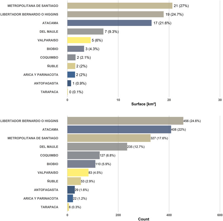
Figure 2. Surface area and number of glacierets by region. In parentheses, the percentage of the total is shown. Regions are shown from the largest to the smallest area and number of glacierets.

2.2 Visual inspection of glacierets with surface less than 0.01 km²

The IPG2022 methodology DGA (2022) establishes that all “new” glaciers (those not included in the previous glacier inventory, IPG2014) had to have a surface area greater than or equal to 0.01 km². Nonetheless, glaciers with a surface less than 0.01 km², and down to 0.001 km², were included if they had already been inventoried in the IPG2014 (Barcaza et al., 2017). In this sense, according to DGA (2022), a very small glacieret (with a surface between 0.001 km² and 0.01 km²) was included in the IPG2022 if it fulfilled either one of the following conditions: (1) the glacier was individually mapped in the IPG2014 and persisted in the IPG2022 with a surface area between 0.001 and 0.01 km², or (2) the glacier had fragmented from a larger glacier mapped in the IPG2014. Considering that there are approximately 8 years between the IPG2014 and IPG2022 and that rapid mass loss has been observed for glacierets in the Swiss Alps in recent decades (Fischer et al., 2014), we expect that the very small glacierets in our study area have also experienced recent mass loss. We also expect that, due to their particularly small surface (below 0.01 km²) most of these very small glacierets have vanished in the years after their mapping as part of the IPG2022. In order to test these hypotheses, a detailed on-screen inspection was conducted for all 588 glacierets whose surface area is between 0.001 and 0.01 km² in the IPG2022 within our study area (Figure 1).

The 588 small glacierets analysed represent 31.68% of the total glacierets within the study area. We employed high-resolution imagery available on ESRI basemaps, Google Earth Pro platform, and PlanetScope data, which were utilised to analyse the presence or absence of visible surface ice (Table 1). The inspection was conducted intensively, one by one for each glacieret, comparing manually all available sources in parallel. The high-resolution images allowed us to accurately assess the surface characteristics of very small glacierets over 5 years from 2018 to 2023. Nevertheless, in some instances, imagery from 2024 was also employed to corroborate their status. We chose this 5-year period as it represents the minimum established time for an ice mass to continuously endure to qualify as a glacier by the IPG2022. If the ice mass was not recognisable in one of the images, then it would be a snow patch instead of a glacier according to this criteria (DGA, 2022).

Table 1

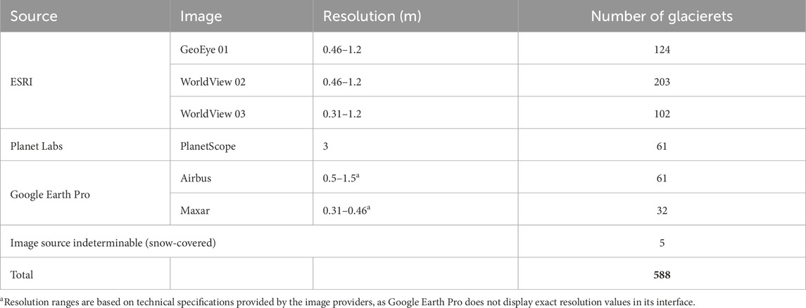
Table 1. Summary of images used to analyse 588 glacierets smaller than 0.01 km².

Considering all available imagery, and after the visual on-screen inspection throughout the IPG2022 glacier outlines, all the 588 very small glacierets, with a surface between 0.001 km² and 0.01 km², were classified into three categories: visible surface ice, non-visible surface ice (when either bedrock or regolith was observed instead of ice), and undetermined. This classification was based on the presence or absence of visible ice. In cases where all available imagery showed an extended snow cover over the glacieret, we classified it as undetermined (Figure 3). A further classification was applied to the non-visible surface ice category. When bedrock or waterbeds were observed, the classification “entirely vanished” was applied, and when regolith was observed, “presumably vanished” was applied. In the latter case, the morphological context of the analysed glacieret’s location was also considered: When it was surrounded by slopes with potential debris input, the likelihood that the ice was covered, rather than having completely vanished, increased. This interpretation was based on visual evidence obtained from the high-resolution satellite imagery used, as well as the analysis of local geomorphology. Although this approach carried a certain degree of uncertainty, the subcategorisation enabled a higher level of confidence in determining whether a small glacierets had completely vanished or, to a lesser extent, whether its surface was potentially covered by debris.

Figure 3

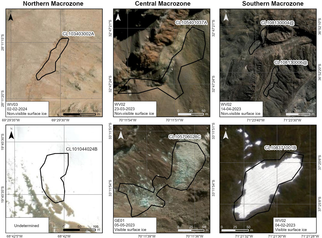
Figure 3. Examples of classification of glacierets into three categories based on visual inspection: visible surface ice, non-visible surface ice, and undetermined. Glacieret’s codes are derived from the IPG2022.

2.3 Glacier surface albedo

Glacier surface albedo is one of the most critical factors in quantifying the radiative forcing and, thus, assessing glacier surface mass balance. Additionally, it can help assess the amount of debris cover and its changes over time. Surface albedo is defined as the proportion of solar radiation reflected by the Earth’s surface compared to the incident solar radiation, and it is expressed by Equation 1:

$\alpha =\frac{S{W}_{\text{ref}}}{S{W}_{\text{in}}}(1)$

Where $S{W}_{\text{ref}}$ is the reflected shortwave radiation, and $S{W}_{\text{in}}$ is the incoming shortwave radiation.

Broadband albedo, also known as shortwave (SW) albedo, is the ratio of reflected flux density (W/m²) to incident flux density across the full solar spectrum $(0.3\text{–}3\mu \text{m})$. In contrast, narrowband albedo refers to reflectivity over specific wavelength ranges. Estimating surface albedo using satellite data can be achieved through various methods, including narrow-to-broadband conversion and angular modelling of the bidirectional reflectance distribution function (BRDF).

Broadband surface albedo $\alpha$ was estimated using a narrow-to-broadband conversion (Bonafoni and Sekertekin, 2020). This method converts the Bottom of Atmosphere (BOA) reflectances measured in specific spectral bands (narrow bands) into a representative broadband albedo estimate. This approach achieves a spatial resolution of 10 m and has shown high accuracy for albedo estimation, particularly in cloud-free Sentinel-2 observations.

The broadband surface albedo $\alpha$ is estimated by the integration of narrowband reflectances across the shortwave (SW) spectrum as expressed by Equation 2:

$\alpha ={\displaystyle \sum _{B=1}^B}{\rho }_B\cdot w_B(2)$

Where ${\rho }_B$ is the Bottom of Atmosphere (BOA) reflectance for a specific band $B$ of the SW spectrum, and $w_B$ are the weighting coefficients. The specific bands and their corresponding weighting coefficients used in this study are presented in Table 2.

Table 2

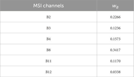
Table 2. MSI spectral bands (similar for Sentinel-2A and -2B) and weighting coefficients $w_B$.

To detect recent changes in surface albedo, we analysed Sentinel-2 images from two time periods: 2019–2020 and 2022–2023. We used images from December to March for both time periods. All image filtering and processing were performed in Google Earth Engine (GEE). To facilitate the visual comparison of albedo conditions inside and outside the glacieret boundaries, a 500-m buffer was applied around each glacieret. We used the buffer to qualitatively show the contrast between the glacieret’s surface and its surroundings (Figure 4).

Figure 4

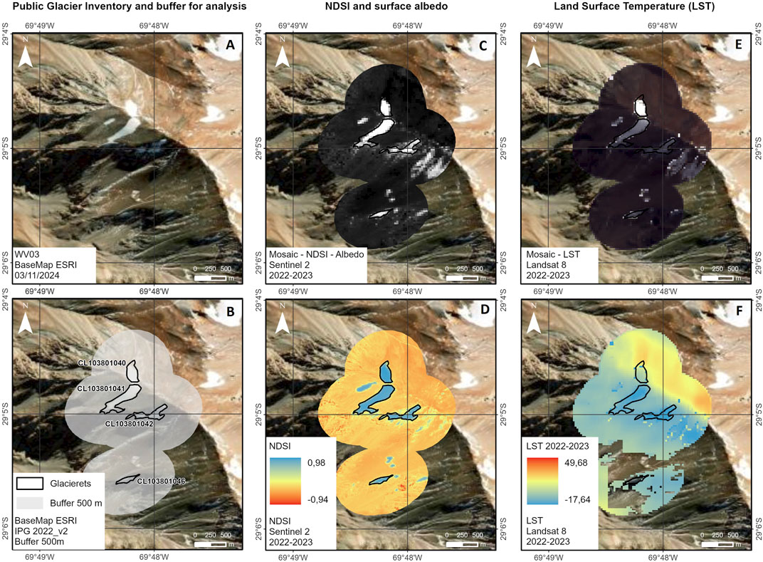
Figure 4. Workflow for glacieret analysis. The process includes: (1) the Public Glacier Inventory (IPG2022_v2) and the defined buffer for analysis [Panels (A,B)]; (2) calculation of the Normalised Difference Snow Index (NDSI) and surface albedo from Sentinel-2 mosaics [Panels (C,D)]; and (3) estimation of Land Surface Temperature (LST) using Landsat 8 data [Panels (E,F)].

Annual composites were generated by selecting the best-available images with minimal cloud cover $(<10\%)$, prioritising those with the fewest pixels showing exposed snow or ice. For discriminating surfaces with visible ice or snow, we used the Normalised Difference Snow Index (NDSI, Equation 3):

$\text{NDSI}=\frac{{\rho }_{\text{GREEN}}-{\rho }_{\text{SWIR}}}{{\rho }_{\text{GREEN}}+{\rho }_{\text{SWIR}}}(3)$

Although previous studies have suggested NDSI thresholds between 0.3 and 0.6 (Durán-Alarcón et al., 2015; Singh et al., 2021), we adopted a conservative empirical threshold of 0.4 for this study to better distinguish surfaces with visible ice or snow. Thus, for all the 1,856 glacierets within the study area, we calculated the clean ice area as the sum of all Sentinel-2-derived NDSI pixels that meet the following criteria: (1) had a value over the 0.4 threshold, (2) fall within the IPG2022 glacier outlines, and (3) have passed all prior image selection and NDSI filtering steps. Pixels meeting these three conditions were assumed to represent visible surface ice. Surface albedo was calculated then at two different scales: (1) at the pixel level, preserving the 10-m native resolution of Sentinel-2, and (2) as arithmetic mean values per glacieret. This dual-scale approach enabled the evaluation of detailed spatial patterns and broader trends across different glacierets in the study area.

2.4 Glacier surface temperature

As another independent measurement of the extension change of debris cover for all the studied glacierets, we assessed changes in Land Surface Temperature (LST) in a 3 years period, comparing Landsat 8 images from December to March of 2019–2020 and 2022–2023 periods, the driest months of the hydrological year in Chile. The analysis included a buffer of 500 m around each glacieret to visually compare surface thermal results inside and outside the glacieret contours. In this way, results can be validated visually (Supplementary Figure S1).

The analysis to derive LST was performed on Google Earth Engine, using Landsat 8 images for both periods from the collection, which have built-in atmospheric correction (USGS Landsat 8 Level 2, Collection 2, Tier 1). The images used have a resolution of 30 m for optical (B2, B3, B4) and near-infrared/shortwave infrared bands (B5 or NIR, B6 or SWIR1), and 100 m for the thermal band (B10 or TB).

Mosaics were built with the images by selecting up to four images with two principal filters. Firstly, we choose images with the lowest cloud coverage $(<10\%)$, as indicated by the image properties. Secondly, we considered those images with the fewest pixels with exposed snow or ice cover within the glacier boundary.

The LST was estimated by applying the inverse Planck Equation 7 to convert radiance to temperature, which is based on the surface’s emissivity (EM) (Equation 6). The emissivity was calculated using the vegetation fraction (FV) (Equation 5) derived from the Normalised Difference Vegetation Index (NDVI) (Equation 4) as has been done before, including for glaciers in the Andes and the Alps (Durán-Alarcón et al., 2015; Roy and Bari, 2022; Gadekar et al., 2023; Gök et al., 2024). The NDVI index is considered because vegetation has a higher emissivity (0.99) compared to rock or sedimentary surfaces (0.986), meaning vegetated areas tend to have a lower temperature than rock surfaces under the same emitted energy. Although glacierets do not have vegetation on their surface, the areas surrounding them might (e.g., Maule, Ñuble or Biobío regions in the southern margin of the study area).

Based on visual inspection and the results of Lo Vecchio et al. (2018), a temperature variation threshold of $\pm$ 4°C is defined. Variations above 4°C are considered an increase in temperature, while those below −4°C are considered a decrease.

$\text{NDVI}=\frac{{\rho }_{\text{NIR}}-{\rho }_{\text{RED}}}{{\rho }_{\text{NIR}}+{\rho }_{\text{RED}}}(4)$

$\text{FV}={\left(\frac{\text{NDVI}-{\text{NDVI}}_{\min }}{{\text{NDVI}}_{\max }-{\text{NDVI}}_{\min }}\right)}^2(5)$

$\text{EM}=0.004\times \text{FV}+0.986(6)$

$\text{LST\hspace{0.17em}}\left[\text{°C}\right]=\frac{\text{TB}}{1+\left(0.00115\times \left(\frac{\text{TB}}{1.438}\right)\right)\times \ln \left(\text{EM}\right)}-273.15(7)$

As a summary, the three previously developed stages complement the overall workflow for the glacieret analysis (Figure 4). These include: (1) the visual inspection of glacierets with a surface area smaller than 0.01 km², carried out to validate their presence and morphological characteristics; (2) the calculation of surface albedo using Sentinel-2 mosaics, which allows for the assessment of snow surface reflectance; and (3) the estimation of glacier surface temperature based on Landsat 8 thermal imagery, aimed at identifying relevant thermal patterns. Together, these stages enhance the multivariable characterisation and enable a more accurate evaluation of the current state of glacierets. Lastly, we determined the statistical significance of our results through the p-value Wilcoxon test for most of the glacieret’s sample (Supplementary Table S1) as a function of the NDSI, albedo and LST differences. We complemented this analysis with the graphic representation of the 95% confidence interval for each variable.

2.5 Statistical analysis of bias and confidence intervals

To quantify the bias between two paired samples of the same variable (NDSI, albedo and Land Surface Temperature changes) and to assess its statistical significance, a combined approach was implemented, incorporating normality testing, confidence interval estimation, and non-parametric inference.

First, a vector of paired differences (bias) was computed following Equation 8:

$\mathrm{\Delta }=x_{t1}-x_{t0}(8)$

Where $x_{t1},x_{t0}$ represent measurements taken at two distinct time points. The normality of $\mathrm{\Delta }$ was then assessed using the Shapiro-Wilk test. Depending on the result, the appropriate method was selected to compute a 95% confidence interval:

$•$ If normality was assumed $(p>0.05)$, a parametric confidence interval for the mean bias was estimated based on the Student’s t distribution.

$•$ If normality was not supported $(p\le 0.05)$, a non-parametric bootstrap method (percentile bootstrap) was applied to estimate the confidence interval for the median bias, using 1,000 resamples with replacement.

To assess whether the bias was significantly different from zero, the Wilcoxon signed-rank test was performed under the null hypothesis that the median of $\mathrm{\Delta }$ is zero. Then, a histogram of the bias was also generated and annotated with the observed median and confidence interval bounds, enabling a graphical interpretation of the bias magnitude, direction, and associated uncertainty. The results of this analysis are presented as part of the Supplementary Material.

2.6 Meteorological data

Meteorology plays a key role in the energy balance of glaciers, making the analysis of annual mean temperature and precipitation critically important. In this study, annual mean temperature and precipitation data from meteorological stations (647 for precipitation and 379 for temperature) included in the Center for Climate and Resilience Research, CR2, Vismet repository (https://vismet.cr2.cl/) were analysed for two periods: (1) 2000–2023 and (2) 2018–2023. The data was processed using RStudio software. Special emphasis was placed on the 2018–2023 period, as it encompasses the entire visual inspection timeframe for the smallest glacierets, as well as the remote sensing assessment period (southern hemisphere hydrological years 2019 and 2022).

3 Results

3.1 Observed changes on glacierets smaller than 0.01 km²

From the manual on-screen analysis of the 588 glacierets smaller than 0.01 km², 321 glacierets were identified as having no visible surface ice, representing a surface reduction of 1.49 km² (50.83% of total surface) between 3rd February 2020, and 10th April 2024. Of the glacierets without visible surface ice, 244 glacierets were subclassified as underlaid by regolith, 75 by bedrock, and two by water bodies. Considering the possibility of glacierets being covered by debris, the 77 glacierets where we found bedrock, or water bodies, can be considered “entirely vanished,” representing an ice loss of 0.38 km². Meanwhile, the 244 glacierets classified as regolith could be considered “presumably vanished,” representing a potential ice loss of 1.11 km².

Considering the spatial variability of the 321 smallest glacierets identified as having no visible surface ice, the O’Higgins Region exhibited the most significant ice loss in terms of number of “vanished” or “presumably vanished” glacierets, reaching 83.56% (Table 3). This was followed by the Maule Region, with a reduction of 64.95%. Valparaíso and Biobío regions showed similar levels of ice loss, with values of 57.58% and 57.38%, respectively. In contrast, the Metropolitana, Coquimbo, and Antofagasta regions exhibited more moderate losses, with reductions of 40%, 36.14%, and 33.33% in number, respectively. Finally, the Ñuble and Atacama regions recorded the lowest ice loss, at 31.82% and 26.88%, respectively.

Table 3

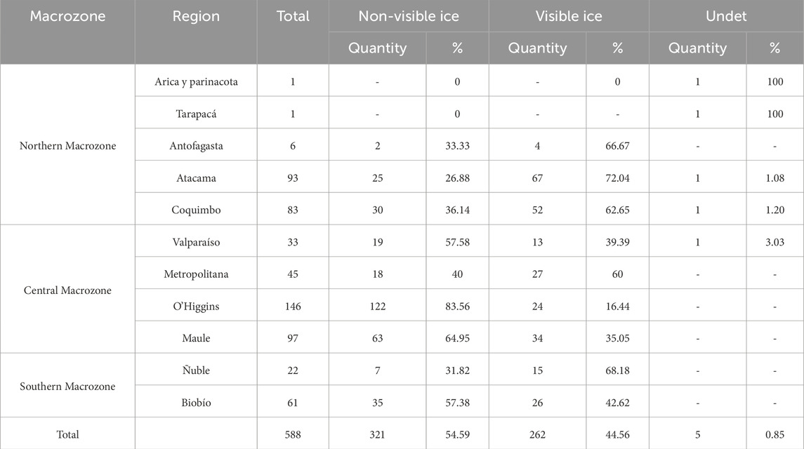
Table 3. Summary of smallest glacierets ($<$0.01 km²) and observed changes for the different regions and macrozones.

Based on the categorisation from the IPG 2022, of the 321 smallest glacierets identified as having “non visible surface ice,” those glacierets with southeast orientation were the most affected by ice loss, accounting for 25.5%, in number, of the total analysed glacierets. This was followed by those with south (23.05%), east (17.13%), and north (8.41%) orientation. The remaining orientations represented a smaller percentage of the total, highlighting the greater vulnerability of those glacierets exposed to solar radiation from the southeast.

Regarding elevation, the 588 analysed glacierets are distributed along an altitudinal belt of 4,527 m, with an average elevation of 3,964 m a.s.l. The average maximum and minimum elevations of the glacierets are 3,987 and 3,940 m a.s.l., respectively. These data indicate a concentration of glacierets within a relatively narrow elevation range, although the extremes reach 2,086 and 6,613 m a.s.l. As for those smallest glaciers entirely, or presumably vanished, we observe a widespread distribution throughout their elevation range of 2,200–6,200 m a.s.l. (Supplementary Figure S2). Nonetheless, there is a large cluster of vanished glaciers below 3,700 m a.s.l. around 34°S and 35°S, with nearly one-third of the whole subsample of vanished small glacierets.

3.2 Glacierets characteristics along the study area

Here, we present the main characteristics of the 1,856 glacierets recognised in our study area according to the IPG2022 and our obtained results through the remote sensing assessment. Although the IPG2022 mentioned in their methodology that the amount of debris on the surface is assessed (DGA, 2022), none of the 1,856 glacierets recognised in our study area have information about the degree of debris cover.

In this regard, when assessing the median NDSI of the glacierets (Figure 5), we found regional differences that are worth mentioning and could help to assess the surface characteristics of Chilean glacierets better. Those at lower elevations (below 5,000 m a.s.l) in the Central macrozone have the lowest NDSI in 2020 and 2023. This pattern is independent of the glacierets’ size; thus, these ice bodies could likely be considered partially or entirely debris-covered, a feature shared by those smallest glacierets, as shown in section 3.1. However, the highest NDSI is shown in those glacierets at higher elevations in the Central and Southern macrozones, which could also indicate clean surface ice (Figure 5). Although, due to the small size of the glacierets, the spatial resolution of the satellite images used here (10 m), and the time difference between the mapping date (average of the year 2017 according to the IPG2022), it is possible that not all the pixels assessed in our analysis are part of the glacierets. Instead, edge effects due to glacier extensional variations could be involved, as discussed in Section 4.1.

Figure 5

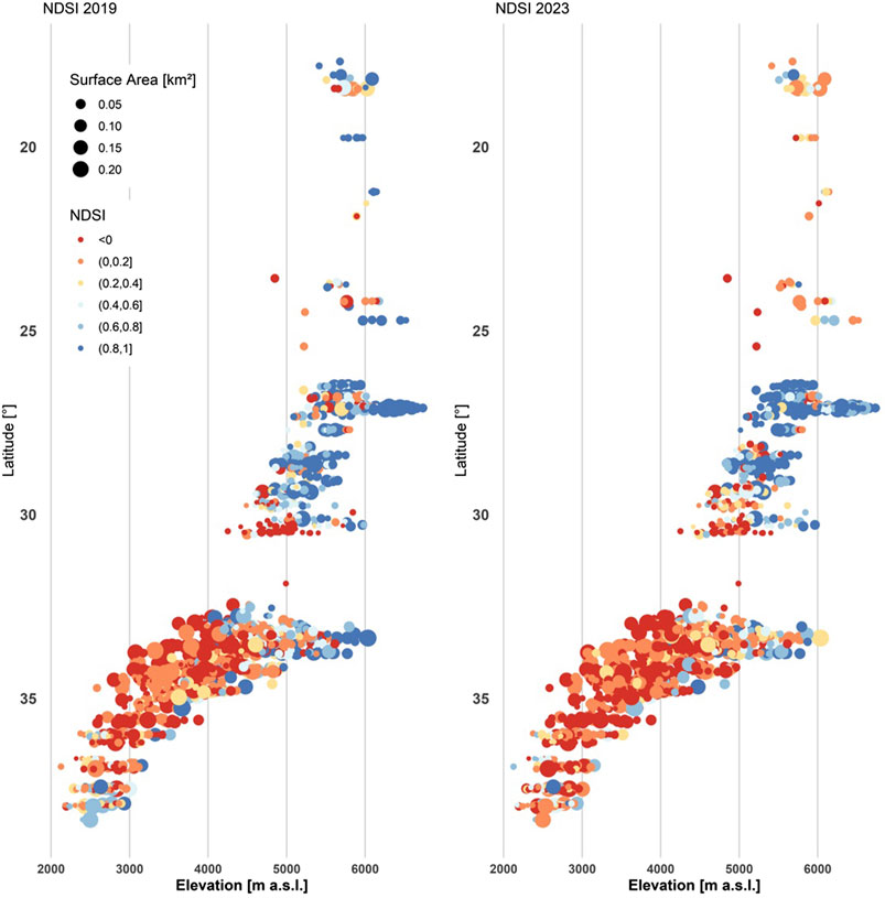
Figure 5. Median NDSI latitudinal and altitude distribution for glacierets in the study area in 2019 and 2023.

Also, we assess the presence of pixels with NDSI $>$ 0.4 for the 1,856 glacierets. We found that 34.75% of the sample (645 glacierets) doesn’t have any pixel with an NDSI higher than 0.4 and, thus, could be considered as totally debris-covered in both the 2019 and 2023 analysed years. This subsample of glacierets with all of their NDSI pixels below 0.4 represents a debris-covered surface of 18.1 km². They also have the lowest median NDSI, and are primarily concentrated in the Central and Southern macrozones (Figure 5). On the contrary, glacierets with pixels with NDSI $>$ 0.4 are also those with higher median NDSI values and are found in the Northern and Central macrozones, mostly above 5,000 m a.s.l. peaks, such as prominent peaks and volcanoes on the Altiplano and in the semi-arid Andes (Atacama, Coquimbo, Valparaíso and Metropolitana regions). We observe another large concentration of glacierets with NDSI pixels over 0.4, along with a high median NDSI, around 33.3°S near 6,000 m a.s.l., corresponding to the Tupungato Volcanic Complex (Figure 5).

Considering the presence of pixels with NDSI $>$ 0.4 for the 1,856 glacierets along the different macrozones and regions, we assess the change in the extent of clean ice between 2019 and 2023. The clean ice area identified by the NDSI threshold is only 37.8% of the total glacierets area and had a reduction of 16.5% between 2019 and 2023. The reduction in area is considerable in the Central macrozone, where 3.84 km² of clean ice has been lost between 2019 and 2023 (Table 4).

Table 4

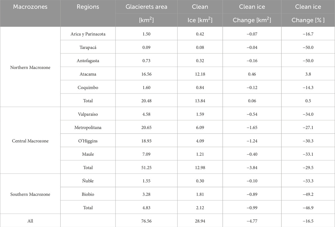
Table 4. Changes in clean ice surface area (NDSI $>0.4$) for glacierets by macrozone and region between 2019 and 2023.

The different regions of the Central macrozone show a general reduction in the clean ice area, ranging from 27.1% in the Metropolitana Region to 34.0% in the Valparaíso Region, with an overall decrease of 29.5% for the whole Central macrozone. Although the extent of the area covered by glacierets is small in the Northern macrozone, some regions, such as Tarapacá and Antofagasta, experienced a reduction of 50% in the extent of clean ice. In contrast, the Atacama Region, which has the greatest extent of clean ice in the Northern macrozone, shows a slight increase of 3.8% between 2019 and 2023, likely related to the presence of snow in the 2023 images. Meanwhile, in the Southern macrozone, the Biobío Region experienced the most considerable relative reduction of clean ice, with a decrease of 49.2%. This contributed to an overall reduction of 46.9% in clean ice area for the analysed portion of the Southern macrozone (Table 4).

3.3 Surface albedo

To assess the satellite-derived albedo between 2019–2020 and 2022–2023, we split the glacierets subset in two: those with and without NDSI pixels greater than 0.4 (Figures 6, 7). Glacierets with NDSI’s pixels lower than 0.4 are more common at lower elevations in the Central Macrozone, showing lower albedo values and no change in albedo between 2019–2020 and 2022–2023 (Figure 6). Meanwhile, those with NDSI pixels greater than 0.4 are present along all the different regions and show the highest albedo values, particularly in the southern margin of the Northern macrozone (Figure 7). Although no general changes are detectable, there are regions where a decrease in albedo between 2019–2020 and 2022–2023 is observed. For example, the highest glacierets of the Northern macrozone show an albedo decrease around 0.3, with a local concentration of this trend evidenced in the Atacama Region. This is also observed in some of the regions of the Central Macrozone, such as the O’Higgins and Valparaíso regions (Figure 8). Overall, the Northern macrozone shows the highest albedo variability mostly concentrated on those glacierets above 5,500 m a.s.l., whereas the Central macrozone shows a similar pattern, mostly for its northern portion in the Coquimbo Region and over 4,000 m a.s.l. (Figure 7).

Figure 6

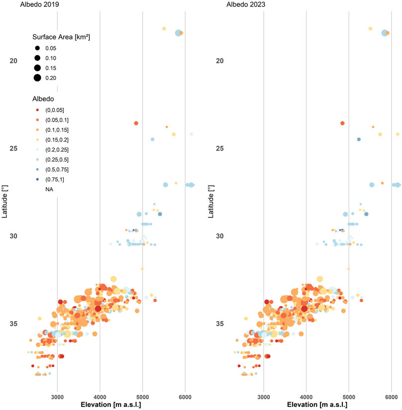
Figure 6. Median albedo of glacierets with NDSI$<$0.4 for the ablation seasons of 2019 and 2023.

Figure 7

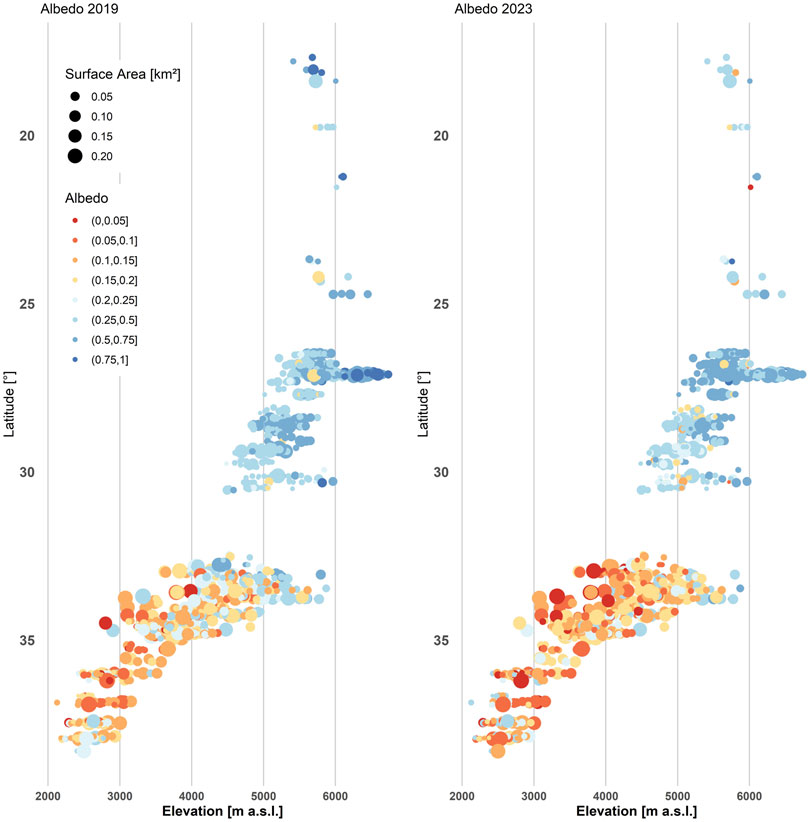
Figure 7. Median albedo of glacierets with NDSI$>$0.4 for the ablation seasons of 2019 and 2023.

Figure 8

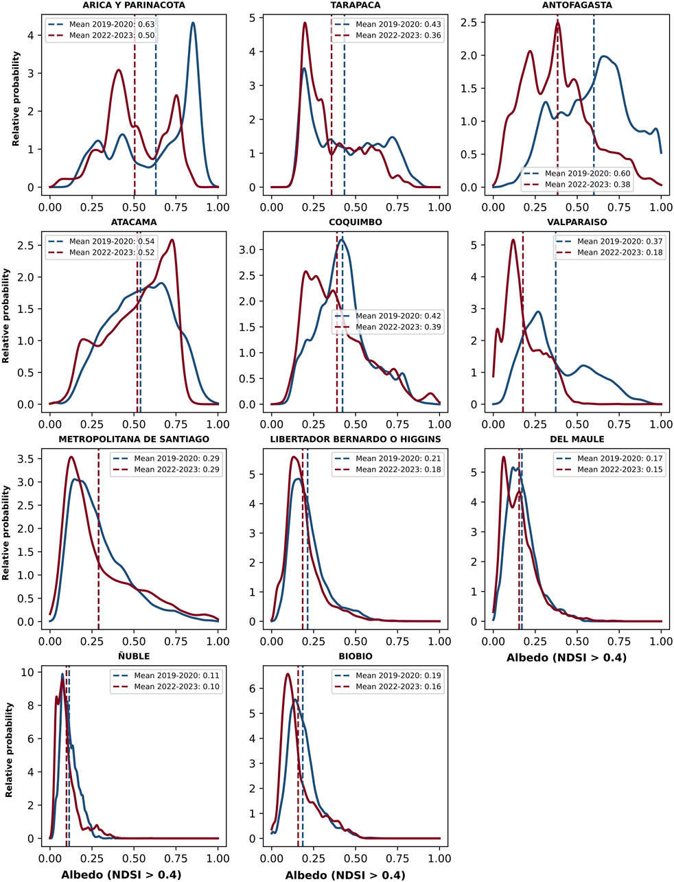
Figure 8. Relative probability distribution of the median albedo for glacierets across Chilean regions, with at least one NDSI pixel over 0.4, comparing data from 2019 to 2020 (blue) and 2022–2023 (red). Vertical dashed lines represent the arithmetic mean temperature value for each region and year.

On a regional basis, we observe a general decrease of the mean albedo for the glacierets located at Arica y Parinacota, Tarapacá, Antofagasta, Coquimbo, Valparaíso, O’Higgins, and Biobío regions (Figure 8). On the other hand, this trend is not clearly observed for the Atacama, Metropolitana, Maule and Ñuble regions. In the particular case of the Atacama Region, Northern macrozone, we observed a heterogeneous trend for the albedo change, as the glacierets in this region have an elevation range of over 2,000 m along with a latitudinal range of 4°. In other cases, when the glacierets are comprised within a short latitudinal range, such as the case of the O’Higgins Region (34°S to 35°S), we observe an albedo distribution with no apparent changes between the periods 2019–2020 and 2022–2023. However, this is not the case for the Valparaíso Region, where, besides an albedo reduction of 0.2, the mean albedo for the 2022–2023 period is far more concentrated towards values under 0.5 (Figure 8).

3.4 Land surface temperature

Land surface temperature for the assessed glacierets ranges between −10°C and 40°C. Higher temperatures are observed, mostly, at lower elevation glacierets, in particular for the year 2023 for those glacierets whose NDSI pixel values were below 0.4 (Figure 9), whereas lower temperature values are observed for those glacierets with at least one pixel with NDSI values over 0.4 located at higher elevations, above 6,000 and 5,000 m a.s.l., for the Northern and Central macrozones, respectively (Figure 10). As for the rest of the glacierets, we do not observe other clear temperature variation trends through their latitudinal and elevation range, independently of their NDSI values.

Figure 9

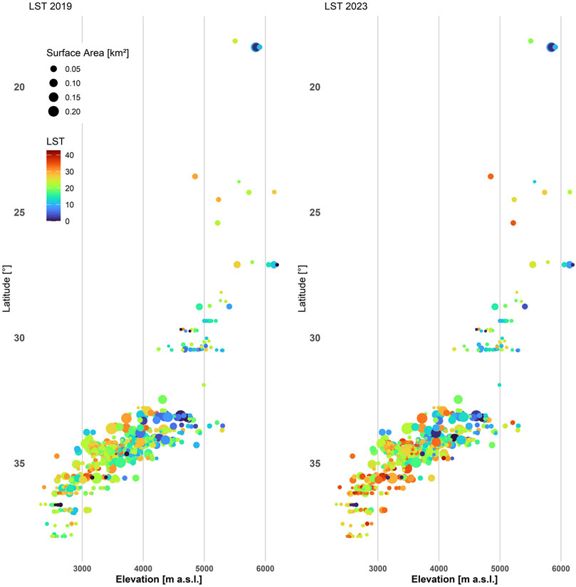
Figure 9. Median land surface temperature of glacierets with NDSI$<$0.4 for the ablation seasons of 2019 and 2023.

Figure 10

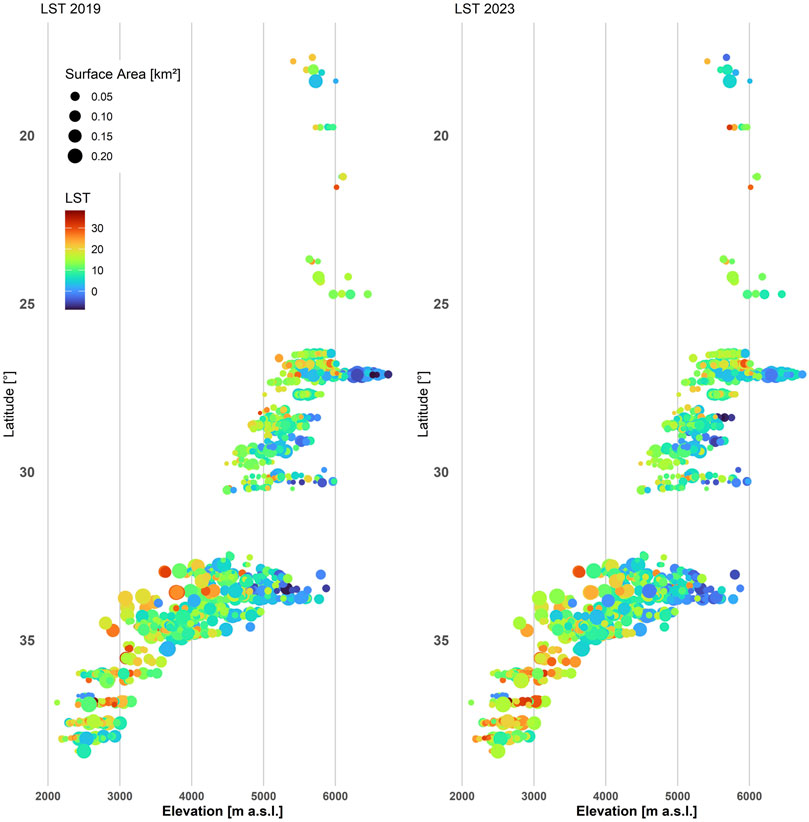
Figure 10. Median land surface temperature of glacierets with NDSI$>$0.4 for the ablation seasons of 2019 and 2023.

Overall, a high range of temperature values is observed along the different regions (Figure 11). In this regard, a positive land surface temperature variation is observed mostly at the Southern macrozone (Ñuble and Biobío regions) with increases ranging between 5°C and 10°C (Figure 11). Particularly, the Biobío Region stands out, with 83% of the glacierets recording increases greater than 4°C. As for the land surface temperature variability in other regions, we observe a slight temperature increase of 1.5°C for the Maule and O’Higgins regions. However, this trend is not clearly observed for those regions ranging from the Metropolitana Region northwards.

Figure 11

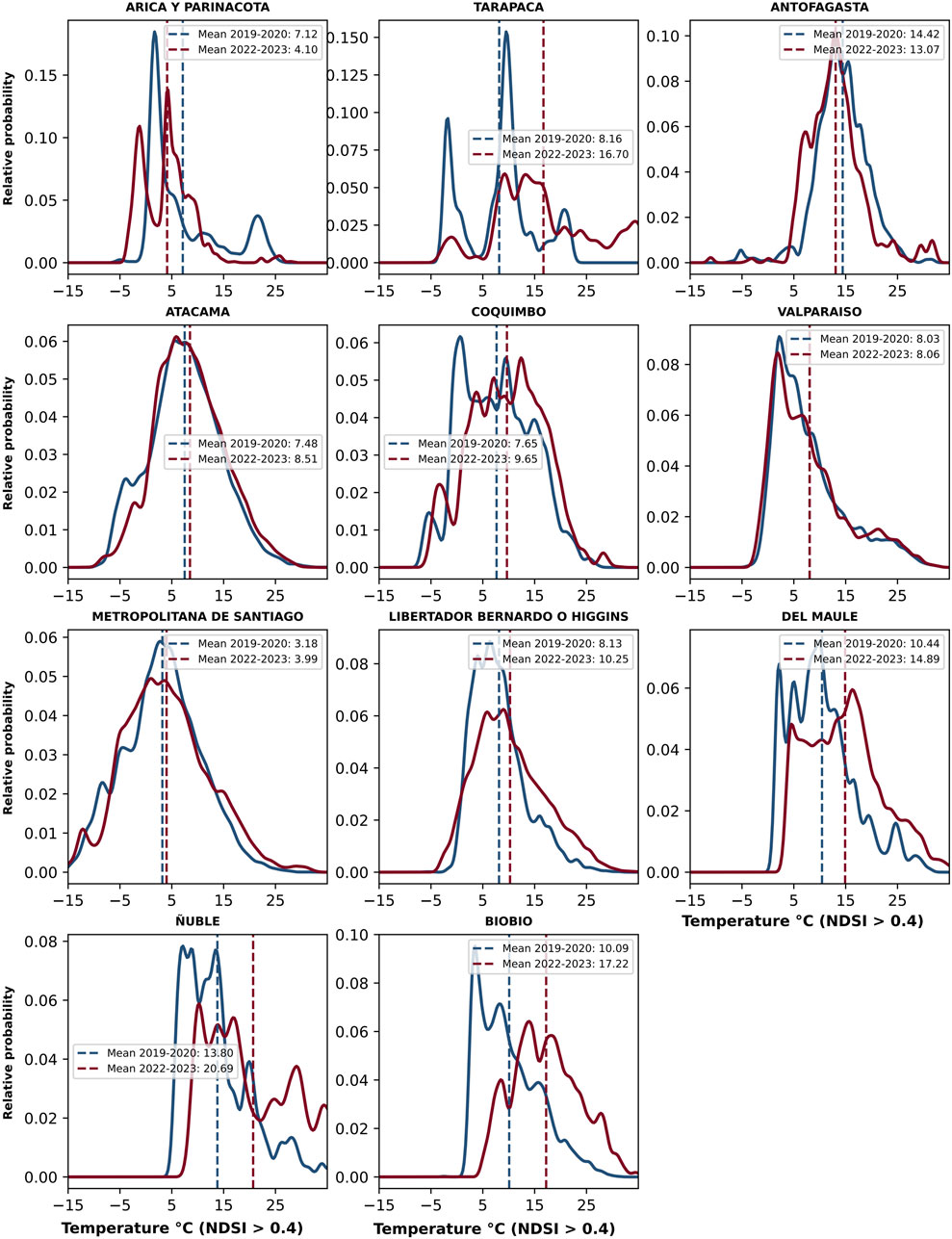
Figure 11. Relative probability distribution of pixel-level land surface temperature values for glacierets across Chilean regions, with at least one NDSI pixel over 0.4, comparing data from 2019 to 2020 (blue) and 2022–2023 (red). Vertical dashed lines represent the arithmetic mean temperature value for each region and year.

3.5 Temperature and precipitation changes

The annual mean temperature for the historical period (2000–2023) ranges from −1°C in the mountainous regions to over 20°C in the coastal and valley areas (Figure 12A). During the 2018–2023 period (Figure 12B), no clear temperature trend is observed, with stations showing both increases and decreases ranging between −1°C and 1°C across the region (Figure 12C). In contrast, over the past 5 years, an overall decrease has been observed across the study area (Figure 12F), except in the mountainous region north of 20°S. This could be explained by the predominance of convective rainfall in that area (Viale et al., 2019), where rising temperatures enhance its occurrence. In the rest of the country, decreases of up to 80% are observed in the mountain range from 30°S southward.

Figure 12

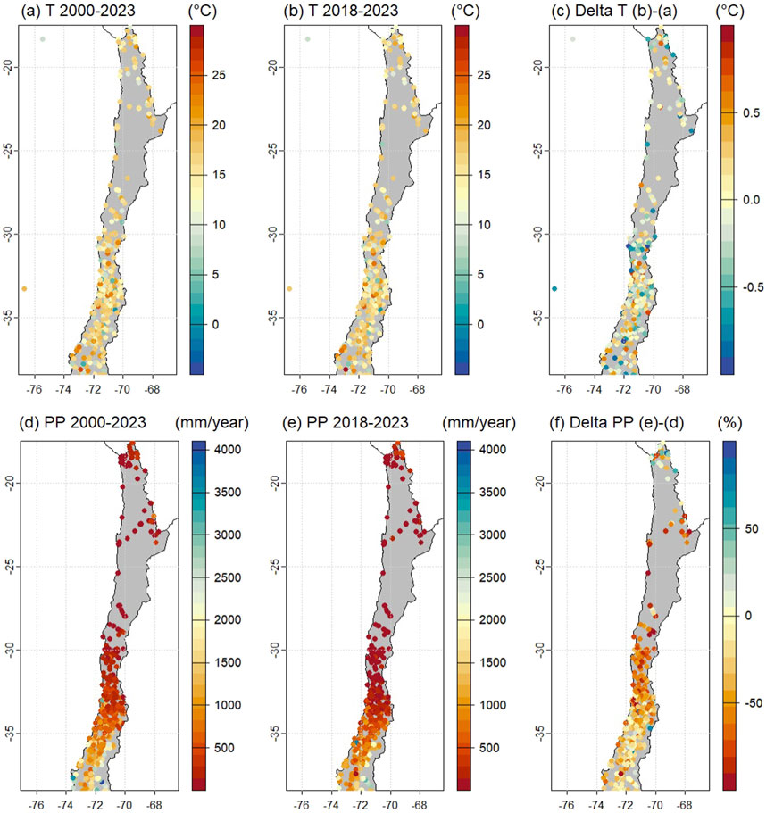
Figure 12. Annual temperature and precipitation changes derived from meteorological station data for the 2000–2023 and 2018–2023 periods. (a): Annual mean temperature for the 2000-2023 period. (b): Annual mean temperature for the 2018-2023 period. (c): temperature changes between 2000-2023 and 2018-2023 periods. (d): Annual mean precipitation for the 2000-2023 period. (e): Annual mean precipitation for the 2018-2023 period. (f): precipitation changes between 2000–2023 and 2018–2023 periods.

4 Discussion

4.1 Methodological limitations

This research confronts several methodological limitations that require careful consideration to interpret its results properly. Among the primary constraints identified are edge effects, glacieret morphology, shadow effects, and the presence of clouds and seasonal snow.

As for the manual inspection of the 588 glacierets with an area smaller than 0.01 km², this method relied primarily on satellite imagery, which inherently introduces a margin of error due to the lack of direct field validation (Paul et al., 2013), despite using the highest available spatial resolution for the images (Table 1). This limitation is particularly evident in the subcategorisation of “presumably vanished” for regolith beds. Such classification should be confirmed through field visits, considering that the morphological context suggests a high likelihood of the surface ice being covered by debris, making it extremely difficult to completely rule out the presence of covered ice in the area. Nonetheless, for those 75 glacierets whose bed material was identified as bedrock, we consider their vanishment as very likely during the 2018–2023 observed period.

Edge effects represent a particularly critical methodological limitation in our analysis. Figure 13 illustrates the relationship between glacieret surface area, as determined by the IPG2022 glacier outlines, and the percentage error associated with area estimation derived from pixel counting (the sum of the area covered by all Sentinel-2 pixels intersecting within the glacieret’s outlines minus the area derived from the IPG2022 outlines expressed as a percentage of the total IPG2022 area). A clear decreasing trend is observed: smaller glacierets $(<0.01k{m}^2)$ exhibit substantially higher relative difference $(>20\%)$, whereas larger areas show a significant reduction in percentage difference (less than 5%). Negative variation values potentially indicate: (1) absence of available albedo data (NaN values), (2) exclusion due to applied filters like cloud or snow coverage, or (3) insufficient pixel coverage within the glacieret outlines. Conversely, positive values indicate that portions of pixels extend beyond the glacieret delimitation, an effect particularly significant in percentage terms for glacierets of reduced dimensions.

Figure 13

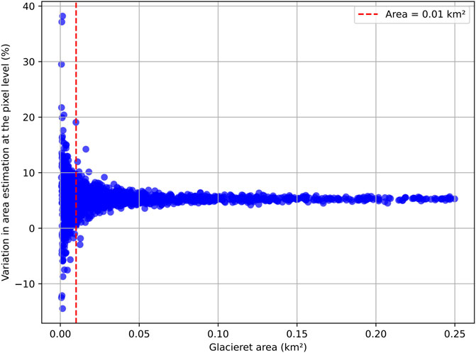
Figure 13. Relationship between glacier area and percentage error in pixel-based area estimation (Sentinel-2 derived albedo, 2022–2023).

This pattern demonstrates the increased impact of spatial discretisation due to raster resolution on small glacier units, where minimal deviations along the glacier boundary represent a considerable proportion of the total area. To address this limitation, particularly for small glacierets, we implemented a control mechanism that included a 500-m buffer zone around each glacieret’s outline 4. This buffer was specifically designed to facilitate a visual comparison between albedo and land surface temperature characteristics inside and outside the glacieret’s boundaries. This comparative approach allowed us to visually confirm that the albedo within the glacieret areas remained distinctly different from the surrounding non-glaciated terrain, despite potential edge contamination.

Several factors impact the accurate estimation of albedo from satellite images. For instance, topographic shadow effects generate a systematic underestimation of albedo in affected areas. On the contrary, snow cover and cloud presence can generate a systematic overestimation of albedo. While we implemented a protocol for selecting images captured during summer to minimise snow presence and ensure that the recorded albedo corresponds primarily to ice, this approach presents additional challenges. In northern regions, the characteristic presence of summer cloudiness incorporates a new source of error. Although we applied specific filters to detect images with minimal cloud coverage, in certain cases, these are insufficient to guarantee the complete absence of clouds over the areas of interest, potentially causing overestimation of albedo. The combined influence of these factors—edge effects, pixel resolution relative to glacieret size, glacieret morphology, topographic shadowing, cloud presence, and ephemeral snow cover demands a nuanced interpretation of the observed albedo patterns and their temporal variations throughout the study period.

Regarding land surface temperature (LST), the study area has a very limited amount of vegetation in the vicinity of glacierets, primarily located between the Maule and Biobío regions. Therefore, the vegetation fraction used for calculating emissivity and LST does not introduce significant first-order influences. Although the work of Gök et al. (2024) in the Alps and Durán-Alarcón et al. (2015) in the Andes demonstrates its valid use over glaciers, considering additional parameters, such as the emissivity difference between ice/snow and debris/rock surfaces, might be appropriate. Nevertheless, omitting this difference is also justified as the ice’s emissivity varies within a narrow range of 0.97–0.99 (Aubry-Wake et al., 2015; Wu et al., 2015). Consequently, we can consider the emissivity of the glacieret’s surrounding rock or debris surface and that of the glacieret itself to be equally 0.98. Nonetheless, considering differential emissivities per material could be a more refined approach for particular cases with more detailed local information.

Additionally, the spatial resolution of the Landsat 8 bands used varies between 30 m for the optical and near/short infrared bands and 100 m for the thermal band (pixel size of 0.01 km²). All glacierets subjected to this analysis have areas smaller than 0.25 km², with 50% of them having smaller areas than 0.18 km². Consequently, the majority of glacierets are primarily covered by fewer than 20 thermal pixels. Furthermore, the 588 glacierets with less than 0.01 km² areas (see Section 3.1) are covered only by 1 pixel. However, given their non-uniform geomorphology, often including elongated lobes, they will have a greater intersection with the surrounding pixels. This leads to a stronger influence from the adjacent material, whether it is snow, water, rock, or debris. For two glacierets of equal area, the one with a more elongated contour will have a greater intersection with the surrounding pixels and, therefore, a greater influence from the adjacent material (see Supplementary Figures S1, S13).

The numerical properties assigned to each glacier (NDSI, Albedo, and LST) use different inputs. The former two are derived from Sentinel 2 images with a 10 m resolution, while LST derived from Landsat 8 images has a spatial resolution of 30 and 100 m. On the other hand, NDSI and Albedo analysis considered the best image from December to March (minimum cloud, shadow and snow coverage). In contrast, LST analysis was based on a mosaic built with the best four images of its corresponding period (March 2020 and March 2023). Therefore, although the images are associated with the same general time period, they don’t correspond to the exact same date or local meteorological conditions. This discrepancy is important to consider when analysing specific cases, such as glacierets exhibiting high albedo values and high temperatures (Figures 7, 10).

The most frequently observed factors that increase the temperature of a glacieret are smaller ice/snow cover, decreased shadow in the image, specific climatic conditions resulting in a higher overall surface temperature, and the number of available pixels in each mosaic. Furthermore, the glacieret’s orientation, area, and shape also influence surface temperature results through solar incidence and the predominant surface type (debris, rock, or ice, Figure 3). While filters for snow and cloud cover were applied, these factors and those mentioned before could not be entirely neglected as they reflect climatic variability resulting from topography, geographic location, daily atmospheric conditions, and image acquisition availability and timing. This leads to varied results across different regions; however, macrozonal trends can still be identified (Figure 11).

Although glacierets with external influences were not excluded due to their large number, LST allows for observing regional-scale trends or variations. Generally, it has been observed that for glacierets with areas greater than 0.05 km², a temperature contrast between the ice surface and the surrounding environment can be observed (Supplementary Figure S1). However, these observations should be complemented with other methods and higher-precision local data. LST alone cannot discern the state of a glacieret, nor its absolute temperature due to external influences unrelated to the glacieret itself. The weak relationship found between low albedo and high temperatures ($R^2<0.2$, see Supplementary Figure S3) suggests the existence of other factors, in addition to debris cover, that exert a positive thermal influence on the results. The temperature trends of the surface adjacent to the glacierets are clearly distinguished by comparing the resulting image and the LST mosaics within the buffer around each glacieret (Figure 4).

4.2 Glacierets characteristics

In terms of the number of glacierets whose surface has at least 100 ${\text{m}}^2$ (one pixel of Sentinel-2 imagery) of visible surface ice (Sentinel-2 derived NDSI pixel values over 0.4), according to the NDSI results (Figure 5), we account for 1,211 glacierets (65.2%) that meet this condition. Although the corresponding accumulated area of this subsample of glacierets is 58.4 km², the estimated clean ice surface, as the sum of all NDSI pixels over 0.4, is only 28.9 km² (Table 4). This surface difference implies that 29.5 km² of the area of the 1,211 glacierets could likely be debris-covered.

Considering that 645 (34.75%) of the 1,856 glacierets have all of their NDSI pixels below 0.4, and, thus, their surface is likely completely covered by debris, we can account, in total, for 47.6 km² of debris-covered surface (62.2%) in the whole glacieret sample. This is the result of the sum between 18.1 km² of all those potentially debris-covered glacierets (Section 3.2; Figure 5) plus the 29.5 km² of debris-covered surface of those glacierets with at least one NDSI pixel over 0.4.

Most of these debris-covered glacierets (81.1% of the subsample) are located in the Central macrozone, mainly below 5,000 m a.s.l. (Figure 5). This feature is consistent with the Central Andes’ rugged relief, favouring the conditions for debris inputs onto glaciers due to mass-wasting process. Such is the case of the large concentration of debris-covered glaciers evidenced on the Central Andes of Argentina (Zalazar et al., 2017). As the IPG2022 doesn’t report information regarding the surface nature of glaciers in Chile (DGA, 2022), we can’t make a similar comparative analysis. As for the Northern and Southern macrozones, we observe that glacierets without visible ice surface are mainly located below 5,000 and 3,000 m a.s.l., respectively, following a similar distribution pattern as observed for the Central macrozone. However, it is worth noting that the Northern and Southern macrozones concentrate only the 12.1% and 6.8% of the potential debris-covered glacierets, respectively. Until a detailed visual inspection of each of the glacierets has been done, it is worth keeping these as “potential” debris-covered glacierets.

Our findings regarding the potential debris-covered glacierets at the lower elevations of each macrozone are consistent with the obtained median albedo values (Figures 6, 7). Lower albedo values (below 0.2) are observed mainly in the Central and Southern macrozones, between 2,100 and 5,000 m a.s.l. In contrast, the Northern macrozone regions present the largest concentration of high albedo values (over 0.4), with 86.8% of their glacierets meeting this condition. This scenario is plausible when considering the smoother terrain for the Altiplano and the semiarid Andes of the Coquimbo Region. This condition has led to the concept of “reservoir glaciers” (Lliboutry, 1956), which implies that a glacier can experience years with either accumulation or ablation throughout its whole extension. Furthermore, the dry, windy, and cold climate of this region makes sublimation the primary process controlling the ablation of these ice masses (Ayala et al., 2017; MacDonell et al., 2013). Although we also observe high albedo values, over 0.4, in the Valparaíso, Metropolitana and O’Higgins regions, the Central macrozone has experienced a more sustained darkening of its glaciers, as discussed in Section 4.2, when compared to the Northern macrozone (Figure 8).

Having a characterisation of the glacieret’s surface features allows us to better understand the mass balance process and its relationship with local climate. Such is the case of a higher albedo of those glaciers in the northern regions, which, besides agreeing with higher NDSI values (Figure 5), matches the lower surface temperatures observed both in 2019 and 2023 (Figure 10). The latter relationship poses significant implications for the energy balance and, thus, the whole mass balance for glacierets.

4.3 Recent changes in glacieret’s surface characteristics

When comparing the extent of the area with NDSI higher than 0.4 between 2019 and 2023, we detect a general reduction of the clean ice area of 16% (Table 4). Nevertheless, the changes are more pronounced at the regional scale, in agreement with the albedo reduction observed in Figure 8, highlighting the impact of the recent drought and increased air temperatures along the Northern and Central macro zones, as observed in Figure 12.

The albedo distribution for each assessed region between 2019 and 2023, as observed in Figure 8, allow us to determine which macrozones experience the most significant albedo fluctuations. In this regard, Figure 14 shows the NDSI, albedo and land surface temperature differences for the whole analysed period (2019–2023 in the case of NDSI and albedo and 2020–2023 for LST) for those glacierets with visible ice surface. Significant negative albedo differences are observed in the northern portion of the Central macrozone (Metropolitana and Valparaíso regions), along with most glacierets of the Arica y Parinacota, Tarapacá and Antofagasta regions. Nonetheless, we also observe a small cluster of negative albedo change on those glacierets above 6,000 m a.s.l. at the Atacama Region. Although the analysis considers only two hydrological years (2019 and 2022), our results agree with the albedo reduction trends constrained by Shaw et al. (2021) of −0.14, on average, for 18 larger mountain and valley glaciers of the Central Andes of Chile (33–34°S) when comparing the year 2020 with the 1986–2009 period.

Figure 14

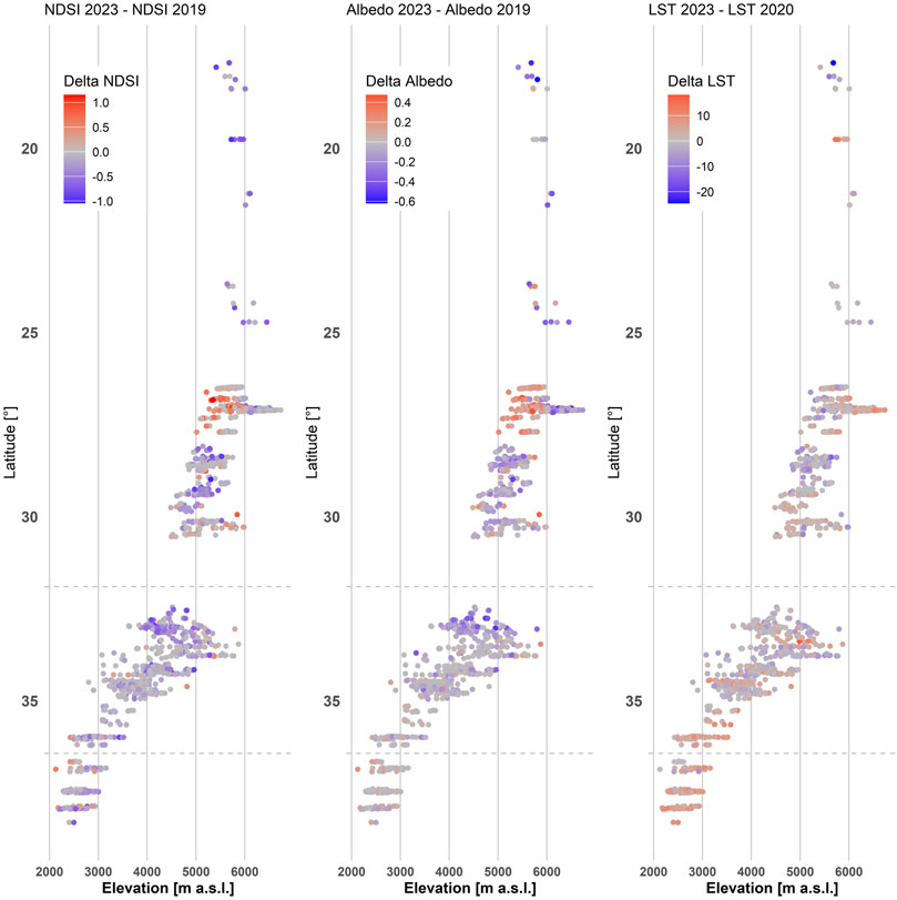
Figure 14. NDSI, albedo and LST changes between 2019 and 2023 for all glacierets with NDSI pixel values greater than 0.4.

These trends are also observed when comparing the same differences for all glacierets larger than 0.01 km² (Supplementary Figures S5, S6). At the same time, this subset of glacierets shows more significant changes than those glacierets with a smaller surface area (Supplementary Figure S13), hence the relevance of the manual inspection. On the contrary, we also observe positive albedo differences for a small subset of glacierets in the Atacama Region between 5,000 and 6,000 m a.s.l. which could be, likely, influenced by the presence of snow cover in the 2023 images (Figure 4), as also revealed by the higher NDSI values on Figure 5. However, this potential positive solid precipitation trend is not clearly observed in the Atacama Region in Figure 12. On the other hand, for those glacierets whose NDSI values report no clean ice (Supplementary Figure S4), we observed the lower albedo values and, at the same time, no significant changes throughout 2019 to 2023 (Supplementary Figures S7, S8).

As a validation assessment, our on-screen analysis of the 588 glacierets smaller than 0.01 km² shows that more than 50% (N = 321), both in quantity and extent, have no visible surface ice or snow on the 2018–2024 period. Considering the characteristics of the surface underlying the glacieret, once no ice is visible, we declare it as “entirely vanished (N = 77)” when it was possible to identify the bedrock and water bodies and “presumably vanished (N = 244)” when we identified the presence of regolith. Thus, we can’t discard those ice bodies as being debris-covered. On a complementary basis, Supplementary Figures S9–S12, show the NDSI, albedo and LST median values, and bias distribution for the small glacierets subset. For the NDSI analysis, we observe a general reduction in the Central and Southern macrozones for the “visible ice” subset (N = 267) (Supplementary Figures S9–S10). As for the “no visible ice” subset (N = 321), we don’t observe significant changes (Supplementary Figures S11–S12), in agreement with lower NDSI values at the beginning of the period due to an already lost ice surface for those “entirely” and “presumably” vanished glacierets. On the other hand, we don’t observe clear changes in albedo and land surface temperature, with the exceptions of the Central macrozone for albedo fluctuations (Supplementary Figure S9) and the Southern macrozone (Ñuble and Biobío regions) for surface temperature variation (Supplementary Figure S9), attributed to the loss of surface ice in those vanished glacierets, in particular for the Biobío Region where 57% (N = 35) of its small glacierets vanished in the last 5 years (Table 3). Such a trend is in agreement with the precipitation decrease observed in Figure 12.

The ice loss within glacierets has led to an average land surface temperature increase across all three macrozones for some specific glaciers. From north to south, notable regions include Tarapacá and Atacama in the Northern macrozone, with increases between 13°C and 15°C; the Metropolitan Region (11°C–14°C) and O’Higgins Region (10°C–11°C) in the Central macrozone; and Ñuble and Biobío regions, where LST has risen between 10°C and 12°C (Supplementary Figures S5–S6). The visual inspection of glacierets with decreasing temperatures does not show any advancement or increase in ice content; the reduction is attributed to external factors, as was discussed in section 4.1. For instance, in the Arica y Parinacota Region, 50% of the glacierets experienced a decrease in average land surface temperature associated with a greater snow cover due to summer precipitation from the Altiplano winter.

In larger glacierets, the expected correlation between areas with temperatures typical of frozen environments (0°C $\pm$ 2°C) and the presence of visible bare ice in the Landsat 8 mosaics is more clearly observed (e.g., glacieret CL103801041@ of 0.09 km², Supplementary Figure S1). In contrast, glacierets with LST exceeding the expected values are also identified, reaching between 30°C and 40°C, ranges consistent with rock or soil surfaces (Brenning et al., 2012; Lo Vecchio et al., 2018; Ren et al., 2024; Liao et al., 2020). This phenomenon suggests the influence of the surrounding debris material adjacent to the glacierets, identified as edge effects, or even the glacieret disappearance, as occurs on some glacierets smaller than 0.01 km², Section 3.1; Supplementary Figures S11–S12. Such temperature trends reflect environmental influences, even when glacierets with decreasing temperatures are excluded. Additionally, we observed that temperatures decrease with glacieret area, with gradients ranging from −52.7°C/${\mathrm{k}\mathrm{m}}^2$ in the north to −22.5°C/${\mathrm{k}\mathrm{m}}^2$ in the south. Studies such as Lo Vecchio et al. (2018) and Ren et al. (2024) suggest validating these results with local data or climatic models like ERA5, especially for smaller areas or large cryoforms with higher thermal resolution.

5 Conclusion

Considering the latest version of the Chilean Public Glacier Inventory, IPG2022, remote sensing, and meteorological stations data, we describe the morphological characteristics of Chile’s glacierets and assess their recent surface changes, including albedo and Land Surface Temperature (LST), from the Arica y Parinacota to the Biobío regions (Desert and Central Andes of Chile). Also, considering the smallest glacierets (those with an extension less than 0.01 km²) included in the IPG2022, we assessed their current status in detail, focusing on the persistence of visible surface ice.

Our study analysed the presence of clean ice for 1,856 glacierets using a threshold of 0.4 for NDSI derived from Landsat 8 (OLI) and Sentinel-2 images between 2019 and 2023. We found that more than 34% of the glacierets could be considered debris-covered, which, at the same time, don’t show significant changes in NDSI between 2019 and 2023, further supporting the hypothesis that their surface is mainly covered by debris. These potential debris-covered glacierets are primarily concentrated in Chile’s Central and Southern macrozones below 5,000 m a.s.l. likely associated with the rugged relief of the Central Andes along with active mass-wasting process. Above 5,000 m a.s.l., we found that glacierets with clean ice and high median NDSI values are more common in the Northern and Central macrozones. In terms of ice loss, we detect a general reduction of the clean ice area of 16%, equivalent to a surface ice loss of −4.77 km² for the 2019–2023 period. Such changes are more pronounced at the regional scale, highlighting the impact of the negative precipitation trends along the Northern and Central macrozones.

Our analysis of albedo changes shows that those glacierets with no clean ice have lower albedo values and thus don’t show significant changes. Meanwhile, glacierets with clean ice have the highest albedo values and, at the same time, manifest a slight albedo decrease in the Central and Southern macrozones, in concordance with the shrinkage of the clean ice surface. The land surface temperature changes between 2019 and 2023 show positive regional trends for most glacierets within the study area, particularly those in the Southern macrozone (Biobío and Ñuble regions).

Our on-screen analysis of the 588 glacierets smaller than 0.01 km² included in the IPG2022 shows that more than 50% (N = 321), quantity and extent, had no visible surface ice by 2023–2024. Considering the characteristics of the exposed glacier bed, we declare 77 glacierets as “entirely vanished” when bedrock or water bodies were exposed, and 244 glacierets as “presumably vanished” for those glacierets underlaid by regolith. Thus, we can account for an ice loss of up to 1.49 km² directly linked to the vanishment of those glacierets that already had an ongoing reduction trend.

The glacieret’s surface changes accounted for in this study are supported by the precipitation reduction trends observed from the meteorological station’s data. In fact, the last 5 years (2018–2023) have been drier than in previous decades (2000–2023), with decreases of up to 80% in mountainous areas.

We hope our analysis of the characteristics and recent changes of these small ice masses helps to better assess their future response to climate change. Our results and discussion represent a valuable contribution to local and regional hydrological assessments, particularly for regions in the Desert and Central Andes of Chile already subjected to hydrological stress.

Data availability statement

The raw data supporting the conclusions of this article will be made available by the authors, without undue reservation.

Author contributions

FU: Conceptualization, Data curation, Formal Analysis, Investigation, Methodology, Visualization, Writing – original draft, Writing – review and editing. HV-A: Formal Analysis, Investigation, Methodology, Visualization, Writing – original draft. MT: Formal Analysis, Investigation, Methodology, Visualization, Writing – original draft. JC: Formal Analysis, Investigation, Methodology, Visualization, Writing – original draft. LR: Formal Analysis, Investigation, Supervision, Validation, Writing – original draft. AA: Formal Analysis, Visualization, Writing – original draft. DP: Formal Analysis, Investigation, Methodology, Visualization, Writing – original draft. CM: Funding acquisition, Resources, Supervision, Validation, Writing – original draft.

Funding

The author(s) declare that financial support was received for the research and/or publication of this article. The study was supported by Geoestudios. The Sentinel satellite images were provided by the Copernicus mission of the European Space Agency. Landsat satellite images were provided by the United States Geological Survey’s (USGS) Earth Explorer interface (https://glovis.usgs.gov/). Diego Pinto received additional support from ANID-PIA Project AFB230001 (AMTC).

Acknowledgments

The authors would like to thank Geoestudios for operational support. We also acknowledge Planet Ⓒ Education and Research Program for their support in providing valuable imagery for our study.

Conflict of interest

Authors FU, HV-A, MT, JC, LR, AA, and CM were employed by Geoestudios, Las Vertientes.

The remaining author declares that the research was conducted in the absence of any commercial or financial relationships that could be construed as a potential conflict of interest.

The authors declare that this study received funding from Geoestudios. The funder had the following involvement in the study: interpretation of data, supervision and formal discussion.

Generative AI statement

The authors declare that no Generative AI was used in the creation of this manuscript.

Publisher’s note

All claims expressed in this article are solely those of the authors and do not necessarily represent those of their affiliated organizations, or those of the publisher, the editors and the reviewers. Any product that may be evaluated in this article, or claim that may be made by its manufacturer, is not guaranteed or endorsed by the publisher.

Supplementary material

The Supplementary Material for this article can be found online at: https://www.frontiersin.org/articles/10.3389/feart.2025.1565290/full#supplementary-material

References

Aceituno, P. (1996). Elementos del clima en el Altiplano Sudamericano. Rev. geofísica 37–55, 44.

Google Scholar

Arias, P., Bellouin, N., Coppola, E., Jones, R., Krinner, G., Marotzke, J., et al. (2021). “Technical summary,” in Climate change 2021: the physical science basis. Contribution of working group I to the sixth assessment report of the intergovernmental panel on climate change. Editors V. Masson-Delmotte, P. Zhai, A. Pirani, S. Connors, C. Péan, S. Bergeret al. (Cambridge, United Kingdom and New York, NY, USA: Cambridge University Press). doi:10.1017/9781009157896.002

CrossRef Full Text | Google Scholar

Aubry-Wake, C., Baraer, M., McKenzie, J. M., Mark, B. G., Wigmore, O., Hellström, R. Ã., et al. (2015). Measuring glacier surface temperatures with ground-based thermal infrared imaging. Geophys. Res. Lett. 42, 8489–8497. doi:10.1002/2015GL065321

CrossRef Full Text | Google Scholar

Ayala, Ã., Farías-Barahona, D., Huss, M., Pellicciotti, F., McPhee, J., and Farinotti, D. (2020). Glacier runoff variations since 1955 in the Maipo River basin, in the semiarid Andes of central Chile. Cryosphere 14, 2005–2027. doi:10.5194/tc-14-2005-2020

CrossRef Full Text | Google Scholar

Ayala, A., Pellicciotti, F., Peleg, N., and Burlando, P. (2017). Melt and surface sublimation across a glacier in a dry environment: distributed energy-balance modelling of Juncal Norte Glacier, Chile. J. Glaciol. 63, 803–822. doi:10.1017/jog.2017.46

CrossRef Full Text | Google Scholar

Barcaza, G., Nussbaumer, S. U., Tapia, G., Valdés, J., García, J.-L., Videla, Y., et al. (2017). Glacier inventory and recent glacier variations in the Andes of Chile, South America. Ann. Glaciol. 58, 166–180. doi:10.1017/aog.2017.28

CrossRef Full Text | Google Scholar

Boisier, J. P., Rondanelli, R., Garreaud, R. D., and Muñoz, F. (2016). Anthropogenic and natural contributions to the Southeast Pacific precipitation decline and recent megadrought in central Chile. Geophys. Res. Lett. 43, 413–421. doi:10.1002/2015GL067265

CrossRef Full Text | Google Scholar

Bonafoni, S., and Sekertekin, A. (2020). Albedo retrieval from Sentinel-2 by new narrow-to-broadband conversion coefficients. IEEE Geoscience Remote Sens. Lett. 17, 1618–1622. doi:10.1109/LGRS.2020.2967085

CrossRef Full Text | Google Scholar

Braun, M. H., Malz, P., Sommer, C., Farías-Barahona, D., Sauter, T., Casassa, G., et al. (2019). Constraining glacier elevation and mass changes in South America. Nat. Clim. Change 9, 130–136. doi:10.1038/s41558-018-0375-7

CrossRef Full Text | Google Scholar

Brenning, A., Peña, M. A., Long, S., and Soliman, A. (2012). Thermal remote sensing of ice-debris landforms using ASTER: an example from the Chilean Andes. Cryosphere 6, 367–382. doi:10.5194/tc-6-367-2012

CrossRef Full Text | Google Scholar

Carrasco, J. F., Osorio, R., and Casassa, G. (2008). Secular trend of the equilibrium-line altitude on the western side of the southern Andes, derived from radiosonde and surface observations. J. Glaciol. 54, 538–550. doi:10.3189/002214308785837002

CrossRef Full Text | Google Scholar

Carvalho Resende, T., Stepanov, M., Bosson, J.-B., Emslie-Smith, M., Farinotti, D., Hugonnet, R., et al. (2022). World heritage glaciers: sentinels of climate change. Tech. Rep. ETH Zurich. doi:10.3929/ETHZ-B-000578916

CrossRef Full Text | Google Scholar

Chen, J., and Ohmura, A. (1990). “Estimation of alpine glacier water Resources and their change since the 1870s,” in I—Hydrology in Mountainous Regions: Hydrologic Measurements, the Water Cycle. Hydrology in Mountainous Regions I. Oslo: International Association of Hydrological Sciences Publication, 193, 127–135.

Google Scholar

Cogley, J., Hock, R., Rasmussen, L. A., Arendt, A. A., Bauder, A., Braithwaite, R. J., et al. (2011). Glossary of glacier mass Balance and related terms, vol. IACS contribution of IHP-VII technical Documents in Hydrology. Paris: UNESCO-IHP.

Google Scholar

Cordero, R. R., Asencio, V., Feron, S., Damiani, A., Llanillo, P. J., Sepulveda, E., et al. (2019). Dry-season snow cover losses in the Andes (18°–40°S) driven by changes in large-scale climate modes. Sci. Rep. 9, 16945. doi:10.1038/s41598-019-53486-7

PubMed Abstract | CrossRef Full Text | Google Scholar

DGA (2022). Metodología del inventario pãšblico de glaciares, sdt N°447. Tech. Rep. SDT N°447, Minist. Obras Públicas, Dirección General Aguas Unidad Glaciol. Nieves., Chile.

Google Scholar

Durán-Alarcón, C., Gevaert, C. M., Mattar, C., Jiménez-Muñoz, J. C., Pasapera-Gonzales, J. J., Sobrino, J. A., et al. (2015). Recent trends on glacier area retreat over the group of Nevados Caullaraju-Pastoruri (Cordillera Blanca, Peru) using Landsat imagery. J. S. Am. Earth Sci. 59, 19–26. doi:10.1016/j.jsames.2015.01.006

CrossRef Full Text | Google Scholar

Dussaillant, I., Berthier, E., Brun, F., Masiokas, M., Hugonnet, R., Favier, V., et al. (2019). Two decades of glacier mass loss along the Andes. Nat. Geosci. 12, 802–808. doi:10.1038/s41561-019-0432-5

CrossRef Full Text | Google Scholar

Falvey, M., and Garreaud, R. D. (2009). Regional cooling in a warming world: recent temperature trends in the southeast Pacific and along the west coast of subtropical South America (1979–2006). J. Geophys. Res. Atmos. 114. doi:10.1029/2008JD010519

CrossRef Full Text | Google Scholar

Farías-Barahona, D., Vivero, S., Casassa, G., Schaefer, M., Burger, F., Seehaus, T., et al. (2019). Geodetic mass balances and area changes of echaurren Norte Glacier (central Andes, Chile) between 1955 and 2015. Remote Sens. 11, 260. doi:10.3390/rs11030260

CrossRef Full Text | Google Scholar

Fischer, M., Huss, M., Barboux, C., and Hoelzle, M. (2014). The new Swiss Glacier Inventory SGI2010: relevance of using high-resolution source data in areas dominated by very small glaciers. Arct. Antarct. Alp. Res. 46, 933–945. doi:10.1657/1938-4246-46.4.933

CrossRef Full Text | Google Scholar

Florentine, C., Harper, J., Fagre, D., Moore, J., and Peitzsch, E. (2018). Local topography increasingly influences the mass balance of a retreating cirque glacier. Cryosphere 12, 2109–2122. doi:10.5194/tc-12-2109-2018

CrossRef Full Text | Google Scholar

Gadekar, K., Pande, C. B., Rajesh, J., Gorantiwar, S. D., and Atre, A. A. (2023). “Estimation of land surface temperature and urban heat island by using Google Earth engine and remote sensing data,” in Climate change impacts on natural Resources, ecosystems and agricultural systems. Editors C. B. Pande, K. N. Moharir, S. K. Singh, Q. B. Pham, and A. Elbeltagi (Cham: Springer International Publishing), 367–389. doi:10.1007/978-3-031-19059-9_14

CrossRef Full Text | Google Scholar

Garreaud, R. D. (2009). The Andes climate and weather. Adv. Geosciences (Copernicus GmbH) 22, 3–11. doi:10.5194/adgeo-22-3-2009

CrossRef Full Text | Google Scholar

Garreaud, R. D., Boisier, J. P., Rondanelli, R., Montecinos, A., Sepúlveda, H. H., and Veloso-Aguila, D. (2020). The Central Chile Mega Drought (2010–2018): a climate dynamics perspective. Int. J. Climatol. 40, 421–439. doi:10.1002/joc.6219

CrossRef Full Text | Google Scholar

Gök, D. T., Scherler, D., and Wulf, H. (2024). Land surface temperature trends derived from Landsat imagery in the Swiss Alps. Cryosphere 18, 5259–5276. doi:10.5194/tc-18-5259-2024

CrossRef Full Text | Google Scholar

Huss, M. (2013). Density assumptions for converting geodetic glacier volume change to mass change. Cryosphere 7, 877–887. doi:10.5194/tc-7-877-2013

CrossRef Full Text | Google Scholar

Huss, M., and Fischer, M. (2016). Sensitivity of very small glaciers in the Swiss Alps to future climate change. Front. Earth Sci. 4. doi:10.3389/feart.2016.00034

CrossRef Full Text | Google Scholar

Izagirre, E., Revuelto, J., Vidaller, I., Deschamps-Berger, C., Rojas-Heredia, F., Rico, I., et al. (2024). Pyrenean glaciers are disappearing fast: state of the glaciers after the extreme mass losses in 2022 and 2023. Reg. Environ. Change 24, 172. doi:10.1007/s10113-024-02333-1

CrossRef Full Text | Google Scholar

Liao, H., Liu, Q., Zhong, Y., and Lu, X. (2020). Landsat-based estimation of the glacier surface temperature of hailuogou glacier, southeastern Tibetan plateau, between 1990 and 2018. Remote Sens. 12, 2105. doi:10.3390/rs12132105

CrossRef Full Text | Google Scholar

Lliboutry, L. (1956). La mécanique des glaciers en particulier au voisinage de leur front. Ann. géophysique 12, 245.

Google Scholar

Lliboutry, L. (1998). “Glaciers of chile and Argentina,” in Satellite Image Atlas of Glaciers of the World, Geological Survey Professional Paper 1386-I-6. Editor R. Williams, and J. Ferrigno (Reston, VA: USGS).

Google Scholar

Lo Vecchio, A., Lenzano, M., Durand, M., Lannutti, E., Bruce, R., and Lenzano, L. (2018). Estimation of surface flow speed and ice surface temperature from optical satellite imagery at Viedma glacier, Argentina. Glob. Planet. Change 169, 202–213. doi:10.1016/j.gloplacha.2018.08.001

CrossRef Full Text | Google Scholar

MacDonell, S., Kinnard, C., Mölg, T., Nicholson, L., and Abermann, J. (2013). Meteorological drivers of ablation processes on a cold glacier in the semi-arid Andes of Chile. Cryosphere 7, 1513–1526. doi:10.5194/tc-7-1513-2013

CrossRef Full Text | Google Scholar

Masiokas, M., Delgado, S., Pitte, P., Berthier, E., Villalba, R., Skvarca, P., et al. (2015). Inventory and recent changes of small glaciers on the northeast margin of the Southern Patagonia Icefield, Argentina. J. Glaciol. 61, 511–523. doi:10.3189/2015jog14j094

CrossRef Full Text | Google Scholar

Masiokas, M. H., Cara, L., Villalba, R., Pitte, P., Luckman, B. H., Toum, E., et al. (2019). Streamflow variations across the Andes (18°–55°S) during the instrumental era. Sci. Rep. 9, 17879. doi:10.1038/s41598-019-53981-x

PubMed Abstract | CrossRef Full Text | Google Scholar

Masiokas, M. H., Christie, D. A., Le Quesne, C., Pitte, P., Ruiz, L., Villalba, R., et al. (2016). Reconstructing the annual mass balance of the Echaurren Norte glacier (Central Andes, 33.5°S) using local and regional hydroclimatic data. Cryosphere 10, 927–940. doi:10.5194/tc-10-927-2016

CrossRef Full Text | Google Scholar

Masiokas, M. H., Rabatel, A., Rivera, A., Ruiz, L., Pitte, P., Ceballos, J. L., et al. (2020). A review of the current state and recent changes of the andean cryosphere. Front. Earth Sci. 8, 99. doi:10.3389/feart.2020.00099

CrossRef Full Text | Google Scholar

Parkes, D., and Marzeion, B. (2018). Twentieth-century contribution to sea-level rise from uncharted glaciers. Nature 563, 551–554. doi:10.1038/s41586-018-0687-9

PubMed Abstract | CrossRef Full Text | Google Scholar

Paul, F., Barrand, N. E., Berthier, E., Bolch, T., Casey, K., Frey, H., et al. (2013). On the accuracy of glacier outlines derived from remote sensing data. Ann. Glaciol. 54, 171–182. doi:10.3189/2013AoG63A296

CrossRef Full Text | Google Scholar

Ramírez, E., Francou, B., Ribstein, P., Descloitres, M., Guérin, R., Mendoza, J., et al. (2001). Small glaciers disappearing in the tropical Andes: a case-study in Bolivia: glaciar Chacaltaya (16o S). J. Glaciol. 47, 187–194. doi:10.3189/172756501781832214

CrossRef Full Text | Google Scholar

Ren, S., Yao, T., Yang, W., Miles, E. S., Zhao, H., Zhu, M., et al. (2024). Changes in glacier surface temperature across the Third Pole from 2000 to 2021. Remote Sens. Environ. 305, 114076. doi:10.1016/j.rse.2024.114076

CrossRef Full Text | Google Scholar

Roy, B., and Bari, E. (2022). Examining the relationship between land surface temperature and landscape features using spectral indices with Google Earth Engine. Heliyon 8, e10668. doi:10.1016/j.heliyon.2022.e10668

PubMed Abstract | CrossRef Full Text | Google Scholar

Shaw, T. E., Ulloa, G., Farías-Barahona, D., Fernandez, R., Lattus, J. M., and McPhee, J. (2021). Glacier albedo reduction and drought effects in the extratropical Andes, 1986–2020. J. Glaciol. 67, 158–169. doi:10.1017/jog.2020.102

CrossRef Full Text | Google Scholar

Singh, D. K., Thakur, P. K., Naithani, B. P., and Kaushik, S. (2021). Quantifying the sensitivity of band ratio methods for clean glacier ice mapping. Spatial Inf. Res. 29, 281–295. doi:10.1007/s41324-020-00352-8

CrossRef Full Text | Google Scholar

UNESCO/IASH (1970). “Perennial ice and snow masses: a guide for compilation and assemblage of data for a world inventory,” in A2486 of technical papers in Hydrology (Paris: UNESCO/IASH).

Google Scholar

Veettil, B. K., and Kamp, U. (2019). Global disappearance of tropical mountain glaciers: observations, causes, and challenges. Geosciences 9, 196. doi:10.3390/geosciences9050196

CrossRef Full Text | Google Scholar

Viale, M., Bianchi, E., Cara, L., Ruiz, L. E., Villalba, R., Pitte, P., et al. (2019). Contrasting climates at both sides of the Andes in Argentina and Chile. Front. Environ. Sci. 7, 69. doi:10.3389/fenvs.2019.00069

CrossRef Full Text | Google Scholar

WGMS (2021). Global Glacier change bulletin No. 4 (2018-2021). Zurich, Switzerland: World Glacier Monitoring Service. zemp, m., gärtner-roer, i., nussbaumer, s. u., hüsler, f., machguth, h., mölg, n., paul, f., and hoelzle, m. (eds.), icsu(wds)/iugg(iacs)/unep/unesco/wmo. edn. 00000.

Google Scholar

Wu, Y., Wang, N., He, J., and Jiang, X. (2015). Estimating mountain glacier surface temperatures from Landsat-ETM Â + thermal infrared data: a case study of Qiyi glacier, China. Remote Sens. Environ. 163, 286–295. doi:10.1016/j.rse.2015.03.026

CrossRef Full Text | Google Scholar

Zalazar, L., Ferri, L., Castro, M., Gargantini, H., Giménez, M., Pitte, P., et al. (2017). Glaciares de Argentina: Resultados Preliminares del Inventario Nacional de Glaciares Glaciers of Argentina: Preliminary Results of the National Inventory of Glaciers. Rev. Glaciares Ecosistemas Montaña 2, 13–22.

Google Scholar

Zemp, M., Frey, H., Gärtner-Roer, I., Nussbaumer, S. U., Hoelzle, M., Paul, F., et al. (2015). Historically unprecedented global glacier decline in the early 21st century. J. Glaciol. 61, 745–762. doi:10.3189/2015jog15j017

CrossRef Full Text | Google Scholar