Abstract
Background:
Accurate precipitation forecasting is crucial for various sectors, such as agriculture, hydrology, and disaster management. In recent years, machine learning (ML) techniques have proven invaluable in improving the accuracy of rainfall prediction and identifying the complex relationships between precipitation and other meteorological variables.
Methods:
This paper presents acomprehensive analysis of the use of multivariable statistical and ML models to predict monthly rainfall at 13 locations in the eastern Amazon. Each model is trained separately for each month, allowing for a tailored representation of precipitation patterns and variations. Additionally, the performance of these models is evaluated via the time series cross-validation technique and an independent test.
Results:
The results indicate that for the points Serra Sul, Açailândia, and Ponta da Madeira, the multivariable models yielded the best monthly performance in 72.23% of the cases, mainly during the rainy season.
Discussion:
Our results highlighted several important aspects of precipitation prediction at different points across the selected study region, particularly concerning the influence of exogenous variables (mainly u10, t2m, TSA, and TNA) on precipitation in most months. Additionally, our findings indicate that the ARIMA, XGBoost, and CNN-1D models outperformed the other models in monthly rainfall forecasting for the Serra Sul, Açailândia, and Ponta da Madeira regions, respectively.
1 Introduction
Precipitation is a natural phenomenon that plays an important role in the hydrological cycle, climate regulation, and maintenance of ecosystems. Precipitation forecasting is crucial for various socioeconomic activities, especially in regions with complex and variable rainfall patterns, such as the Amazon region, where municipalities are strongly affected by extreme floods and droughts that affect river hydrology (Karen et al., 2017; Bauer et al., 2018).
Obtaining meteorological data is essential for making effective rain forecasts, understanding weather patterns, and performing numerical modelling to issue warnings for extreme rainfall events. The most accurate meteorological data records are those measured in situ at weather stations. However, remote regions, such as the Amazon, do not have a high density of weather stations or at least 30 years of data (the minimum period to perform climate studies, according to the World Meteorological Organization). Therefore, it is necessary to choose other meteorological databases. Other types of data, such as 1) gridded data interpolated via measured variables and an interpolation method to create values at each grid point (e.g., Xavier et al., 2022 and GPCC - Schneider et al., 2016); 2) satellite data, from which different variables can be inferred (e.g., IMERG - Sharifi et al. (2016) and CMORPH - Joyce et al. (2004); 3) mixed methods with satellite data and interpolation schemes (e.g., CHIRPS - Funk et al. (2015) and MERGE - Rozante et al. (2020)); and 4) reanalysis data, which result from combining observed data (weather station and satellite data) with numerical modeling results (e.g., ERA5 - Hersbach et al. (2020) and JRA55 - Kobayashi et al. (2015)).
The main subseasonal to seasonal prediction methods are based on statistical and dynamic models (Vitart and Robertson, 2019). Notably, dynamic models yield good predictability at the weather scale (1–10 days), but at the scale used in this paper (subseasonal to seasonal), they do not perform well (Toth and Buizza, 2019). At this temporal scale, forecasts of short-term spatial scale patterns are lost (approximately 15 days are currently available); for example, it is not possible to predict cold fronts, stability lines, etc., and therefore, it is not possible to accurately predict how much rain or how many of temperature fluctuations will occur on a specific day (if it is more than 15 days after day 0). Nevertheless, several large-scale spatial patterns are still predictable (El Niño, La Niña, tropical Atlantic dipole, and Madden-Julian oscillation, among others). Thus, it is possible to predict the trend of an atmospheric or oceanic pattern (if the pattern is above or below the historical average), such as the precipitation or temperature pattern (Toth and Buizza, 2019).
Accurate seasonal predictions are available for tropical South America (Sampaio and Silva Dias, 2014), but subseasonal predictions, such as one-monthly cumulative precipitation, are a new area in the field of meteorological prediction, and only a few centers do such forecasts, with even fewer providing publicly available data (some examples are NMME-USA, CanSIPs-Canada, APCC-South Korea, INMET-Brazil and CPTEC/INPE-Brazil).
As cited above, oceanic patterns are important for predicting monthly precipitation with both dynamic and statistical models. In this work, we choose oceanic phenomena that affect the tropical South American climate: the El Niño-Southern Oscillation (ENSO), Tropical Atlantic gradient (TAG), and South Atlantic gradient (SAG). ENSO is the positive (El Niño) or negative (La Niña) sea surface temperature (SST) anomaly in the equatorial Pacific (Marengo et al., 2012; Tedeschi et al., 2013; Tedeschi and Sampaio, 2022), and TAG is the gradient in SST between northern and southern tropical Atlantic (Nobre and Shukla, 1996; Münnich and Neelin, 2005). Moreover, the SAG is similar to the TAG but in the South Atlantic instead of the Tropical Atlantic (Espinoza et al., 2014; Bombardi et al., 2014).
Some published works have addressed the use of ML and statistical techniques in precipitation prediction or in other correlations between meteorological variables and the occurrence of floods, specifically in some regions of the Amazon. Anochi et al. (2021) compared the results of extreme gradient boosting (XGBoost) with those of deep learning and the Brazilian Global Atmospheric Model to predict precipitation over South America. Meteorological data collected between 1980 and 2016 were used, and the input information for the ML models included precipitation, surface pressure, surface air temperature, 850 hPa air temperature, specific humidity, and zonal and meridional wind components (u10 and v10, respectively). The results indicated that the precipitation predictions for the Amazon region for austral summer and autumn were associated with considerable errors. On the other hand, for the austral winter and spring seasons, the prediction error was minor. Similarly, Alves et al. (2023) presented a method for monthly precipitation forecasting based on an artificial neural network (ANN) and the Group Method of Data Handling (GMDH) with SSTs extracted from monthly precipitation data in a specific area of the municipality of Marabá, located in the southeastern region of Pará state, as the input. After a variable selection step, the intelligent model was used to obtain the mean monthly SST in predefined areas while considering temporal lag. For ANN training, precipitation data from the Climate Prediction Center were used. The results demonstrated the effectiveness of the GMDH method for monthly precipitation prediction. Taveira et al. (2023) addressed the use of a statistical model based on the probability function of the Gamma distribution to calculate the monthly rainfall probability for the municipality of Rio Branco, which is located in the state of Acre, Brazil. The data used to develop the model pertain to monthly precipitation levels from 1970 to 2021, obtained from INMET station 82,915. The model results indicate that, for a 95% probability, the monthly rainfall values ranged from 1.48 to 3.78 mm for the months of June, July, and August (dry season) and between 22.41 and 175.14 mm for the remaining months (rainy season). Most recently, James and Calheiros (2024) investigated the impact of precipitation data balancing on rainfall forecasting for a location in the interior of the state of Amazonas, Brazil. In this study, an ANN model was used to perform hourly rainfall forecasting on the basis of regressive data of this meteorological variable, which were obtained from rain gauge instruments, two disdrometers, and a radiometer. The results of this study, which were conducted with data from 18 February 2022, indicate that the model achieved root mean squared error (RMSE) values between 2.54 and 7.77 for the test data.
Additionally, some published studies have focused on employing machine learning models to predict river flooding in the Amazon region on the basis of precipitation data from various localities. Vieira et al. (2021) explored the prediction of river flooding in the Amazon region. In this work, the authors employed a genetic algorithm to select the meteorological variables most correlated with flooding in the Xingu River Basin, which is located in the state of Pará. Among the analyzed variables were precipitation, SST, and atmospheric pressure at sea level in Darwin and Tahiti. Similarly, Mesquita et al. (2023) investigated the use of ML models for flood forecasting in the Xingu River via precipitation data. This study proposed the use of a convolutional neural network (CNN) fed with recurrence plot (RP) data to forecast floods in the Xingu River. The proposed model utilized monthly precipitation information and maximum effluent levels of the river between 1974 and 2019. The results indicate that the CNN with RP outperforms other ANN-based models, achieving MAE values of 50.74 for the test data. Recently, Filho et al. (2024) developed a model based on an ANN trained with hourly precipitation data and the levels of three effluents to forecast floods in the Branco River, which is located in the Amazon Basin. The rainfall data used were obtained from the PDIRnow model between 2015 and 2022, whereas the effluent data were collected from stations near the rivers. The ANN model achieved RMSE values ranging from 1.27 to 2.18 for a forecasting horizon between 6 and 24 h.
Based on these previous studies, this work presents a novel approach by being the first to statistically evaluate the correlation between multiple meteorological variables and precipitation at selected points in the eastern Amazon. Additionally, this study is the first to investigate a fragmented forecasting strategy, where models are trained separately to predict rainfall for each specific month. By assessing the performance of statistical and machine learning models during both the rainy and dry seasons, this research provides new insights into the predictability of precipitation patterns in the region, advancing beyond previous works in the field.
2 Materials and methods
2.1 Study area
This study was carried out for 13 specific points in the eastern Amazon. Figure 1 shows the studied points and their locations. Some reasons for choosing this region are as follows: 1) the Amazon basin is the largest and one of the most biodiverse places in the world (Nobre et al., 2021), and the East Amazon Basin is especially strongly affected by SST anomalies in the equatorial Pacific and Atlantic (Andreoli et al., 2012; Pezzi and Cavalcanti, 2001; SOUZA et al., 2000); 2) the Itacaiunas Basin has some mining companies operating in it, but many preserved areas also exist; because of this, many studies have been conducted in different areas of the basin (Souza-Filho et al., 2015; 2016; Cavalcante et al., 2020; 2021; Pontes et al., 2022); and 3) one of the largest and most important logistical corridors in Brazilian mining is located in this region.
FIGURE 1

Monthly precipitation climatologies (mean monthly precipitation from 1979 to 2010, unit: mm/month) at each studied point (red points). The bar charts illustrate the seasonal distribution of rainfall, highlighting distinct rainy and dry season patterns between the points located in southeastern Pará and Maranhão.
The Amazon basin is characterized by a tropical climate, specifically, a monsoon regime (two well-defined seasons, on the basis of the quantity of rain). Notably, the rainy and dry seasons occur in different months in different parts of the basin. An analysis of data from the selected points (Figure 1) reveals that the rainy season at southern points occurs between November and April, whereas at northern points it occurs between January and July.
2.2 Data
The studied region does not have official stations weather with a great quantity of data (at least 30 years), in all interested points. So it is necessary to choose some gridded data. The ERA5 (Hersbach et al., 2020) reanalysis was chosen because although it is not the best option for precipitation (Lavers et al., 2022; Jesus et al., 2024; Polasky et al., 2025), this data set contains all the atmospheric and oceanic variables used in this study. And in this case, all variables are in the same earth system. This dataset was created by the European Centre for Medium-Range Weather Forecast (ECMWF). This dataset contains hourly and monthly data and covers the period from 1940 to present. Data for all areas of Earth are available, with grids of different sizes (31 km, 62 km, 0.5°, and 1.0°) and 37 pressure levels (1,000–1 hPa). In this study, only surface (1,000 hPa) and monthly data collected between 1979 and 2022 were used, with a spatial resolution equal to 0.5° in latitude and longitude. The chosen variables were precipitation, SST, zonal and meridional winds (u10 and v10, respectively) at 10 m, and air temperature at 2 m (t2m).
Precipitation is commonly correlated with other atmospheric and oceanic variables (Guo et al., 2014; Djibo et al., 2015). After some initial analysis, we selected u10, v10, and t2m at the prediction points and different SST indices defined by the scientific community on the basis of important oceanic patterns, such as ENSO, TAG, and SAG, for correlation analysis. The indices used were Niño 1+2, Niño 3, and Niño 4 in the equatorial Pacific; Tropical Northern Atlantic (TNA) and Tropical South Atlantic (TSA) in the tropical Atlantic; and North-South Atlantic (NSA) and South-South Atlantic (SSA) oscillations in the Atlantic. The corresponding regions are shown in Figure 2.
FIGURE 2

Oceanic regions used to calculate the indices Niño 1+2, Niño 3, Niño 4, TNA, TSA, NSA, and SSA based on SST anomalies.
2.3 Precipitation prediction pipeline
The proposed computational pipeline used to predict monthly precipitation, illustrated in Figure 3a, involves several sequential stages that encompass preprocessing, time series cross-validation (TSCV), and independent tests. This pipeline can be used to establish forecasting models and assess their performance in predicting monthly precipitation prediction.
FIGURE 3

Proposed pipeline for training the monthly precipitation forecasting models. (a) The general pipeline encompasses preprocessing, TSCV, and independent test stages; (b) Preprocessing stage of the meteorological variables.
The raw data extracted from ERA5 are preprocessed in several steps and conditioned for training monthly forecasting models, as illustrated in Figure 3b. The preprocessed steps do not include analysing the missing values because ERA5 data do not have missing values in their time series. The TSCV is used to evaluate the generalizability of the model and select the best hyperparameter set for each model trained with the dataset for a specific month. Independent tests are employed for each model to evaluate the prediction horizon in reference to the observed data.
In the following subsections, each part of the proposed pipeline is explained in detail.
2.3.1 Preprocessing
The proposed preprocessing stage illustrated in the second box in the pipeline Figure 3a shows in greater detail in Figure 3b. In the preprocessing stage, the raw monthly total precipitation (TP) data extracted from the ERA5 dataset are scaled by converting the data from m/day to mm/month. This conversion is achieved by multiplying the total precipitation by the number of days in the month and by 1,000 (e.g., the TP is multiplied by 31,000 for October months). The processed TP represents the target variable for training the forecasting models.
In parallel, the raw SST data are processed to extract the mean temperatures for the Niño 1+2, Niño 3, Niño 4, TNA, TSA, NSA, and SSA regions. These seven oceanic variables are grouped with t2m, u10, and v10 data to compose the input variable set for training the forecasting models. A one-period lag (f(t-1)) is applied to these input variables to ensure that the TP is predicted with past weather data, as shown in the orange rounded rectangle.
The next step of preprocessing involves joining the input and target data in a single dataset and dividing it by month. Each monthly dataset is then split into training and test datasets. The training dataset encompasses the measurements between the years 1979 and 2010, whereas the test dataset corresponds to the years between 2011 and 2022.
All the steps described above and illustrated in Figure 3b were implemented in the Python 3 language with the Pandas, Numpy, and NetCDF4 packages.
2.3.2 Model selection and evaluation metrics
Following preprocessing, the model selection stage involves implementing TSCV combined with Bayesian optimization, using the monthly training datasets. This strategy selects the best set of hyperparameters for the forecasting models by month. The TSCV method used in the proposed pipeline employes the expanding window approach, where the training fold is expanded over time for k-folds (Vien et al., 2021; Bergmeir et al., 2018).
The Bayesian optimization minimize the average root mean squared error (avRMSE) obtained by all the folds in the TSCV by tuning the model with different combinations of hyperparameters. In this optimization approach, a probabilistic model is used to estimate the relationship between the input parameters and the objective function, and the model that achieves the lowest error given the allowable ranges of hyperparameters is selected (Head et al., 2018).
The avRMSE is calculated with Equation 1, which yields the average error among the validation folds based on the observed and predicted precipitation values.
The RMSE metric used to evaluate the model in each fold of the TSCV and in the independent test is expressed by Equation 2. The mean absolute error (MAE) also is employed to evaluate the performance of the models in the independent test and can be calculated by Equation 3. The observed precipitation is represented by , and is the predicted precipitation for the -th sample of a total of samples, which represents the total number of samples in each validation fold or the total number of samples in an independent test.
To investigate the contributions of meteorological and climatic variables to the models’ prediction, an explainability analysis was conducted using the SHAP (SHapley Additive exPlanations) method. This approach enables the quantification of each variable’s impact on the model outputs, offering insights into spatial and seasonal variations (Liu et al., 2023). The analysis was carried out for different seasons in each region, including summer (January to March), winter (June to August), and transitional periods. Extreme values were identified and examined to assess their implications for meteorological events and potential modeling limitations. This comprehensive approach supports more robust conclusions regarding the interaction between local and global climatic factors.
Model selection via TSCV and Bayesian optimization, the SHAP analysis, as well as the RMSE and MAE metrics calculation were performed via the Python packages Scikit-Time, Sckit-Learn, Scikit-Optimize, and SHAP respectively. The Supplementary Material file provides the hyperparameter ranges employed in the Bayesian optimization of the models.
2.4 Machine learning and statistical models
The forecasting models employed for predicting monthly precipitation include machine learning and autoregressive statistical models. The ML algorithms used are the recurrent neural network (RNN), long short-term memory (LSTM), gated recurrent unit (GRU), one-dimensional convolutional neural network (CNN-1D), and extreme gradient boosting (XGBoost) models. The statistical models used are autoregressive with exogenous inputs (ARX), autoregressive moving average with exogenous inputs (ARMAX), autoregressive integrated moving average with exogenous inputs (ARIMAX), and autoregressive integrated moving average (ARIMA) models.
Each aforementioned model was separately trained and fine-tuned using TSCV to predict rainfall specifically for each month, with monthly training datasets. For instance, RNN and ARIMA were trained to predict rainfall exclusively in January, while RNN and ARIMA were trained to perform the same task exclusively for May.
The ARX and ARMAX models are stationary techniques widely employed in time series analysis. These models aggregate autoregressive characteristics from the series and the information from exogenous inputs (Shumway and Stoffer, 2017; Nelles, 2001). The ARMAX model also includes a moving average process. Equations 4 and 5 express the mathematical structures of the ARX and ARMAX models, respectively. and represent the -dimensional input vector with the exogenous variables and the corresponding random disturbances, respectively. , , and are the -dimensional vectors of model coefficients related to the input vector, autoregressive term, and moving average terms, respectively.
ARIMAX and ARIMA are nonstationary models with aggregated and integrated components in their mathematical formulas (Alsharef et al., 2022; Shumway and Stoffer, 2017; Tangirala, 2015). Equations 6, 7 express the mathematical structures of the ARIMAX and ARIMA models, respectively, where represents the -th derivative of an integrated component.
Figure 4 illustrates the generic architecture of the ML algorithms employed in this work to predict precipitation. The RNN, LSTM, GRU, and CNN-1D models are based on the neural network architectures shown in Figure 4a. RNNs are connectionist models that represent sequential dynamics through cyclic patterns within a node structure, with nodes called recurrent neurons (Lipton et al., 2015). Node decisions are based on the current input and the output from the previous neuron in the network (Salem, 2022).
FIGURE 4

Architecture of ML models. (a) Diagrams of the RNN, GRU, and CNN-1D models; (b) Diagram of XGBoost structure.
The LSTM model has an augmented RNN architecture developed to process time series information using gating signals at memory neurons to control the flow of information and address long short-term dependence and vanishing gradient issues (Yu et al., 2019; Lipton et al., 2015). The controlled flow of information among the memory neurons allows the LSTM model to store various time dependencies with distinct characteristics (Lindemann et al., 2021).
Similarly, the GRU model was introduced by Cho et al. (2014) as an alternative to traditional models; it employs mechanisms that complement time series prediction via improved integration with short-term information (Lindemann et al., 2021). Compared with LSTM, the gated memory neuron of a GRU has a simplified structure based on gating systems that allow past information to be discarded.
CNN-1D is a convolutional neural network architecture designed to handle one-dimensional sequential data and perform tasks such as regression, classification, and feature extraction (Guessoum et al., 2022; Kiranyaz et al., 2021). This algorithm is composed of kernels associated with convolutional layers, pooling layers, and dense fully connected layers, as shown in Figure 4a.
XGBoost is an ensemble ML algorithm that was proposed by Chen and Guestrin (2016) and is used in classification and regression problems. This algorithm groups and trains decision trees via the gradient-boosting method based on the recursive residual of training for consecutive trees to reduce estimation errors (Ali et al., 2023). The output of XGBoost is the average response from each output generated by each trained decision tree Z, as shown in Figure 4b.
The autoregressive and ML models were implemented via the Python packages Scikit-Time, XGBoost, and TensorFlow.
3 Results
The results presented in this section refer to the analysis of precipitation predictions at points Serra Sul (SES), Açailândia (ACA), and Ponta da Madeira (PDM). The results obtained for the remaining 10 points are provided in the Supplementary Material.
3.1 Precipitation prediction for Serra Sul
The results obtained with all the models for the TSCV and the independent test for monthly precipitation prediction in the Serra Sul region are shown in Table 1, and in Figures 5a,b, respectively.
TABLE 1
| Month | ARX | ARMAX | ARIMAX | ARIMA | RNN | LSTM | GRU | CNN-1D | XGBoost |
|---|---|---|---|---|---|---|---|---|---|
| Jan | 109.238 | 107.747 | 155.666 | 83.824 | 133.749 | 258.276 | 152.013 | 125.412 | 87.102 |
| Feb | 226.720 | 225.932 | 167.668 | 112.036 | 184.793 | 130.304 | 183.608 | 85.116 | 83.272 |
| Mar | 88.169 | 90.467 | 139.744 | 89.469 | 120.396 | 148.560 | 114.572 | 108.334 | 72.968 |
| Apr | 92.617 | 92.254 | 125.855 | 87.290 | 83.208 | 135.202 | 86.448 | 76.778 | 78.201 |
| May | 53.968 | 57.967 | 65.424 | 70.673 | 63.191 | 111.559 | 65.405 | 59.050 | 60.264 |
| Jun | 28.568 | 27.897 | 38.139 | 27.866 | 23.35 | 26.189 | 26.940 | 18.406 | 20.427 |
| Jul | 33.925 | 34.329 | 51.475 | 30.261 | 40.288 | 59.683 | 50.120 | 32.807 | 21.286 |
| Aug | 63.993 | 63.428 | 71.495 | 33.273 | 51.662 | 58.893 | 64.298 | 42.072 | 30.108 |
| Sep | 72.234 | 69.681 | 138.102 | 44.093 | 65.712 | 63.116 | 73.085 | 49.068 | 51.698 |
| Oct | 109.060 | 109.89 | 134.503 | 67.271 | 60.733 | 71.494 | 68.866 | 58.004 | 48.416 |
| Nov | 85.052 | 85.427 | 95.287 | 73.448 | 109.922 | 101.976 | 111.014 | 90.171 | 60.990 |
| Dec | 234.049 | 235.674 | 206.617 | 75.993 | 100.882 | 84.340 | 99.809 | 62.285 | 87.916 |
avRMSE results for the TSCV analysis with the models for monthly precipitation prediction at SES.Ṁ
Bold numbers represent the lowest avRMSE value by month.
FIGURE 5
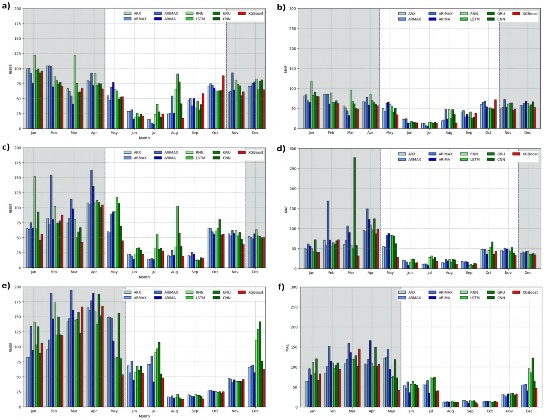
RMSE and MAE values obtained for the models in the independent tests between 2011 and 2022 for the regions SES, ACA, and PDM. (a) RMSE values in SES; (b) MAE values in SES; (c) RMSE values in ACA; (d) MAE values in ACA; (e) RMSE values in PDM; and (f) MAE values in PDM. The gray area indicates the rainy season. The variation of RMSE and MAE in independent test across months and between the rainy and dry seasons is more significant at ACA and PDM than at SES.
A comparison of the results obtained in the two analyses reveals that the XGBoost model predominantly achieves the lowest avRMSE values at the monthly scale, as highlighted in Table 1, with values ranging from 21.286 to 72.968.
An evaluation of the impact of varying time window lengths (TWLs of 3, 4, 5, and 6 months) within the validation fold for March, the month with the most critical rainfall patterns in the SES region, revealed no statistically significant differences in the performance of the ARIMA model. This conclusion is supported by the Kruskal–Wallis test (p-value = 0.9991). The distribution of RMSE values across TWLs is illustrated in Supplementary Figure S1a.
On the other hand, Figure 5a shows that in the independent test, the ARIMA model achieves the lowest RMSE values over 5 months of the year, predominantly displaying the best performance, with values ranging from 7.631 to 77.677 (see Supplementary Table S21). Similarly, the MAE values obtained by ARIMA model show the lowest prediction error in 5 months, with values ranging from 5.536 to 68.524, as shown in Figure 5b. Comparatively, XGBoost achieves optimal performance among the tested models in only 3 months for this location, as indicated in Table 3.
Specifically for the rainy season in Serra Sul (between November and April), the ARIMA model yields RMSE values between 40.847 and 77.677 and MAE values between 32.640 and 68.524 in the independent test, whereas for the dry season (between May and October), the values for RMSE vary between 7.631 and 76.965 and MAE vary between 5.536 and 66.583, with the lowest value occurring in July (see Supplementary Tables S21, S33). Compared with XGBoost, this model achieves a reduction of over 24% in RMSE values for January, February, and March.
The confidence interval analysis shown in Figure 6 indicates that the ARIMA model yielded the most consistent performance in predicting average monthly precipitation for the years between 2011 and 2022. Its estimates are closer to the historical mean (blue bars), indicating higher accuracy. Additionally, it shows the smallest confidence interval among the nine models evaluated, suggesting greater precision, as shown in Figure 6a. This behavior highlights statistical robustness and lower uncertainty in its predictions, while the other models display greater variability and deviate more from the observed values, mainly for the rainy season.
FIGURE 6

Confidence interval analysis of the models prediction by month in SES region. Each plot displays the historical monthly average precipitation (blue bars), the model’s predicted monthly average (solid red line), and the confidence interval of the predictions (shaded red area). The models represented are: (a) ARIMA; (b) ARX; (c) ARMAX; (d) ARIMAX; (e) XGBoost; (f) RNN; (g) LSTM; (h) GRU; and (i) CNN-1D.
The charts in Figure 7 display the observed and predicted rainfall values by the models for the month of March, which recorded the highest historical average for this region between 2011 and 2022. In both charts, it is evident that the ARIMA model showed the lowest prediction variability, in addition to achieving the lowest estimation error for the years 2011, 2012, 2017, and 2022. Meanwhile, the XGBoost model presented the lowest error for the years 2019 and 2020.
FIGURE 7

Observed and predicted values by the models for the month of March from 2011 to 2022 in the SES region. Each panel displays the observed monthly accumulated precipitation values in millimeters per year (gray bars), along with lines and markers representing the predictions of each model. (a) Comparison of the ARIMA model (red line) with the ARX (green line), ARMAX (blue line), ARIMAX (orange line), and XGBoost (purple line) models; (b) Comparison of the ARIMA model (red line) with the RNN (green line), LSTM (blue line), GRU (orange line), and CNN-1D (purple line) models.
A comparative analysis of the monthly rainfall forecasts generated between 2011 and 2020 by the models developed in this study and those produced by multiple linear regression (MLR) models with one- and 2-month lags (MLR-L1 and MLR-L2), commonly employed as baseline forecasting tools by a mining company operating in the study regions (Ferreira et al., 2024), reveals that, during the rainy season in the SES region, the ARX model attained RMSE and MAE values comparable to those of the MLR-L1 and MLR-L2 models, particularly from January through April, as illustrated in Figures 8a,b. During the dry season, there is also consistent evidence that the trained models outperformed the MLR baselines, particularly between May and September.
FIGURE 8

RMSE and MAE values obtained for the MLR-L1, MLR-L2 and trained models in the independent tests between 2011 and 2020 for the regions SES, ACA, and PDM. (a) RMSE values in SES; (b) MAE values in SES; (c) RMSE values in ACA; (d) MAE values in ACA; (e) RMSE values in PDM; and (f) MAE values in PDM. The gray area indicates the rainy season. The variation of RMSE and MAE in independent test across months and between the rainy and dry seasons is more significant at ACA and PDM than at SES.
These findings indicate that, for the analysis between 2011 and 2022, the ARIMA model, which uses only autoregressive values of monthly precipitation, and the XGBoost model yield competitive results compared with the other multivariable models for SES, as these models generalize the monthly precipitation dynamics. The results also indicate that some multivariable models, such as ARX, achieved performance comparable to the baseline tools for predicting monthly rainfall during the rainy season (see Supplementary Tables S36, S37).
3.2 Precipitation prediction for Açailândia
The results of the TSCV and independent test analyses achieved with the models applied for monthly precipitation prediction for the ACA point are shown in Table 2, and in Figures 5c,d, respectively. Table 2 indicates that the ARIMA model yields the lowest avRMSE values for 5 months, with values ranging from 22.722 to 116.020 in the TSCV analysis, whereas XGBoost is the second-best-performing model and displays the optimal performance for 3 months, with avRMSE values between 20.264 and 127.358.
TABLE 2
| Month | ARX | ARMAX | ARIMAX | ARIMA | RNN | LSTM | GRU | CNN-1D | XGBoost |
|---|---|---|---|---|---|---|---|---|---|
| Jan | 100.496 | 101.229 | 132.983 | 80.921 | 148.445 | 132.254 | 145.003 | 108.213 | 98.836 |
| Feb | 196.097 | 193.064 | 260.138 | 116.020 | 177.444 | 131.681 | 147.286 | 116.251 | 104.781 |
| Mar | 120.629 | 119.981 | 159.601 | 81.086 | 181.646 | 141.757 | 282.167 | 146.806 | 127.358 |
| Apr | 86.491 | 87.371 | 100.257 | 95.246 | 130.390 | 131.647 | 136.297 | 127.434 | 113.758 |
| May | 63.341 | 67.180 | 78.616 | 82.694 | 87.127 | 81.431 | 87.483 | 65.316 | 65.728 |
| Jun | 34.822 | 33.592 | 42.605 | 26.966 | 24.644 | 27.059 | 23.503 | 22.524 | 20.264 |
| Jul | 24.592 | 24.788 | 36.472 | 27.233 | 30.819 | 45.448 | 37.026 | 29.406 | 20.874 |
| Aug | 52.234 | 51.897 | 61.294 | 22.722 | 41.395 | 39.459 | 41.879 | 39.631 | 23.256 |
| Sep | 29.972 | 28.630 | 40.200 | 22.846 | 37.191 | 34.673 | 35.446 | 30.625 | 25.145 |
| Oct | 57.785 | 57.938 | 66.739 | 48.462 | 74.396 | 58.647 | 80.310 | 37.740 | 47.025 |
| Nov | 69.523 | 68.841 | 74.423 | 57.715 | 100.36 | 103.297 | 104.441 | 70.426 | 46.696 |
| Dec | 85.582 | 82.659 | 108.099 | 66.516 | 91.273 | 68.470 | 84.210 | 57.609 | 61.985 |
avRMSE results for the TSCV analysis with the models for monthly precipitation prediction at ACA.
Bold numbers represent the lowest avRMSE value by month.
The analysis of different TWLs (3, 4, 5, and 6 months) in the validation fold for March showed that the performance of the XGBoost model remained statistically consistent across all configurations. According to the Kruskal–Wallis test, no significant differences were detected among the different TWLs (p-value = 0.9995). Supplementary Figure S1b displays the RMSE distributions associated with each TWL.
The independent test of monthly forecasts at ACA reveals that the XGBoost model achieves the best performance in 4 months, as shown in Figure 5c where the RMSE values ranging from 15.289 to 104.678 (see Supplementary Table S27). Figure 5d depicts that the MAE values obtained by the XGBoost vary between 11.114 and 98.097 (see Supplementary Table S34). The CNN-1D model yields the second-best results in this analysis and performs best in 3 months, whereas the ARIMA yields the best forecasts only in June and July, as shown in Table 3.
TABLE 3
| Month | SES | ACA | PDM |
|---|---|---|---|
| Jan | ARIMA | CNN-1D | ARX |
| Feb | ARIMA | ARMAX | ARX |
| Mar | ARIMA | XGBoost | CNN-1D |
| Apr | XGBoost | CNN-1D | LSTM |
| May | ARMAX | XGBoost | XGBoost |
| Jun | ARIMA | ARIMA | ARIMA |
| Jul | ARIMA | ARIMA | ARIMA |
| Aug | XGBoost | XGBoost | XGBoost |
| Sep | GRU | GRU | XGBoost |
| Oct | RNN | CNN-1D | CNN-1D |
| Nov | CNN-1D | XGBoost | ARIMAX |
| Dec | XGBoost | ARIMAX | ARIMA |
Best models by month and point according to the independent test results.
Bold numbers represent the lowest avRMSE value by month.
Based on the performance of the models during the rainy season months at this location (between December and April), the CNN-1D model achieved the lowest RMSE value most frequently. The MAE metric shows that CNN-1D also reached the lowest error value for April, while obtained values close to the best for January and December, as shown in Figure 5d. For the dry season (between May and November), the XGBoost model outperforms the other models in 3 months, achieving an RMSE value of 18.840 in August, which is the second-lowest value for this analysis.
The confidence interval analysis for the predictions generated by the models for the Açailândia site, as shown in Figure 9, reveals an interesting pattern when compared to the previously analyzed region. In this case, as illustrated in Figure 9a, the ARIMA model presents lower variability in its predictions; however, the results indicate that both the mean forecast and its confidence interval fail to encompass the historical monthly average for the period between February and May. Conversely, most of the multivariate models present confidence intervals that do include the historical average for each month, with the XGBoost model standing out by providing both predictions and confidence intervals closely aligned with the observed rainfall values, as shown in Figure 9e.
FIGURE 9

Confidence interval analysis of the models prediction by month in ACA region. Each plot displays the historical monthly average precipitation (blue bars), the model’s predicted monthly average (solid blue line), and the confidence interval of the predictions (shaded blue area). The models represented are: (a) ARIMA; (b) ARX; (c) ARMAX; (d) ARIMAX; (e) XGBoost; (f) RNN; (g) LSTM; (h) GRU; and (i) CNN-1D.
An interesting finding that can be abstracted from the results presented in Tables 2, 3 is the type of model that achieved the best performance in each month. For Serra Sul, the ARIMA model clearly performs best; for Açailândia, the multivariable predictive models achieve the best performance in most months for both analyses, which may indicate the contribution that the exogenous meteorological variables make to the explainability of monthly precipitation in this region.
Evaluating the rainfall predictions for the month of March, historically the wettest month in Açailândia between 2011 and 2020, it can be observed that the XGBoost model produced forecasts closest to the observed precipitation values in 50% of the years analyzed (2011, 2012, 2016, 2017, and 2018). Additionally, the model also yielded predictions close to the observed rainfall for the years 2015 and 2021, as illustrated in Figure 10.
FIGURE 10

Observed and predicted values by the models for the month of March from 2011 to 2022 in the ACA region. Each panel displays the observed monthly accumulated precipitation values in millimeters per year (gray bars), along with lines and markers representing the predictions of each model. (a) Comparison of the XGBoost model (red line) with the ARIMA (green line), ARX (blue line), ARMAX (orange line), and ARIMAX (purple line) models; (b) Comparison of the XGBoost model (red line) with the RNN (green line), LSTM (blue line), GRU (orange line), and CNN-1D (purple line) models.
The RMSE and MAE values yielded by the trained models, alongside the baseline models MLR-L1 and MLR-L2, are presented in Figures 8c,d, respectively. These results demonstrate that, during the rainy season in the ACA region from 2011 to 2020, several of the proposed models outperformed the baseline approaches in terms of predictive accuracy. Notably, the best-performing models for the months of January, February, March, and December were XGBoost, ARIMAX, RNN, and ARIMA, respectively. Similarly, during the dry season, improved predictive performance over the MLR-L1 and MLR-L2 models was also observed in specific months (June, July, September, and November) for certain models developed in this study (see Supplementary Tables S38, S39).
3.3 Precipitation prediction for Ponta da Madeira
The results of the TSCV and independent tests with monthly precipitation prediction models trained with the set of meteorological data from the Ponta da Madeira are presented in Table 4, and in Figures 5e,f, respectively.
TABLE 4
| Month | ARX | ARMAX | ARIMAX | ARIMA | RNN | LSTM | GRU | CNN-1D | XGBoost |
|---|---|---|---|---|---|---|---|---|---|
| Jan | 179.101 | 182.33 | 223.783 | 113.681 | 205.263 | 185.233 | 211.475 | 136.613 | 148.746 |
| Feb | 334.393 | 335.567 | 443.908 | 147.035 | 234.135 | 213.267 | 211.105 | 167.194 | 211.810 |
| Mar | 197.037 | 192.481 | 243.688 | 133.513 | 231.832 | 199.622 | 202.632 | 171.31 | 158.075 |
| Apr | 124.336 | 119.198 | 139.656 | 175.389 | 138.418 | 469.34 | 135.331 | 115.057 | 134.462 |
| May | 289.996 | 289.884 | 218.616 | 174.092 | 226.05 | 230.221 | 172.244 | 168.82 | 155.235 |
| Jun | 56.402 | 57.119 | 71.005 | 82.791 | 69.692 | 70.187 | 74.879 | 53.319 | 55.402 |
| Jul | 68.689 | 68.646 | 72.719 | 73.040 | 74.059 | 72.910 | 67.375 | 55.294 | 44.645 |
| Aug | 25.629 | 24.468 | 33.194 | 20.617 | 23.427 | 21.991 | 22.702 | 13.741 | 12.790 |
| Sep | 25.686 | 25.488 | 31.617 | 21.997 | 24.964 | 21.817 | 22.122 | 21.140 | 13.682 |
| Oct | 33.227 | 33.140 | 16.875 | 9.277 | 11.661 | 10.094 | 9.971 | 9.501 | 9.399 |
| Nov | 17.055 | 16.867 | 18.728 | 15.498 | 23.048 | 28.134 | 24.985 | 16.419 | 12.217 |
| Dec | 88.035 | 85.238 | 135.806 | 77.813 | 92.341 | 107.982 | 94.272 | 57.765 | 56.734 |
avRMSE results for the TSCV analysis with the models for monthly precipitation prediction at PDM.
Bold numbers represent the lowest avRMSE value by month.
The TSCV results indicate that the XGBoost model achieves the best performance in forecasting precipitation for 6 months of the year, particularly during the dry season (between June and December) in this region. For the rainy season (between January and May), this same model yields the lowest avRMSE value in May. Additionally, the ARIMA and CNN-1D models yield good predictions in rainy season months.
In the case of the PDM region, the evaluation of different TWLs (3, 4, 5, and 6 months) during the validation phase of TSCV for March revealed statistically significant differences in the performance of the CNN-1D model. The Kruskal–Wallis test confirmed this with a p-value of 0.0004. Among the configurations tested, the TWL of 5 months yielded the lowest avRMSE, indicating superior predictive performance. The validation RMSE values distribution for each TWL for this case is depicted in Supplementary Figure S1c.
With respect to the results obtained in the independent test, the XGBoost and ARIMA models stand out in terms of precipitation forecasting, each equally achieving the best performance in 3 months of the year, particularly during the rainy season in this region (from Jauary to May). The results in Figure 5e indicate that XGBoost yielded RMSE values ranging from 12.764 to 167.813 for monthly prediciton, while ARIMA achieves values between 14.120 and 189.699 over the months (see Supplementary Table S32). Figure 5f shows the analysis of the models based on MAE metric, where the ARIMA obtained values between 10.660 and 166.648, while XGBoost yeilded MAE values between 8.915 and 145.382 (see Supplementary Table S35).
Regarding the variability of monthly predictions for each model, Figure 11 shows that, similar to the other cases, the ARIMA model achieved the narrowest confidence interval compared to the models with exogenous variables, as shown in Figure 11a. However, for some months of the rainy season in Ponta da Madeira, the average predictions of the ARIMA model resulted in higher errors compared to models such as XGBoost, which, despite having a wider confidence interval, produced mean predictions that were much closer to the observed values, as shown in Figure 11e.
FIGURE 11

Confidence interval analysis of the models prediction by month in PDM region. Each plot displays the historical monthly average precipitation (blue bars), the model’s predicted monthly average (solid gren line), and the confidence interval of the predictions (shaded green area). The models represented are: (a) ARIMA; (b) ARX; (c) ARMAX; (d) ARIMAX; (e) XGBoost; (f) RNN; (g) LSTM; (h) GRU; and (i) CNN-1D.
When evaluating the predictions of the models against the observed rainfall values for the month of March in Ponta da Madeira (PDM), a high degree of variability is observed, as shown in Figure 12. This can be attributed to the significant fluctuations in precipitation levels in March throughout the 12-year period. Comparatively, the CNN-1D model demonstrated the best performance for this month, accurately predicting rainfall values close to the observed data for the years 2012, 2013, and 2015. Additionally, for the years 2011, 2017, and 2021, it achieved predictions that were very close to those of the best-performing models.
FIGURE 12

Observed and predicted values by the models for the month of March from 2011 to 2022 in the PDM region. Each panel displays the observed monthly accumulated precipitation values in millimeters per year (gray bars), along with lines and markers representing the predictions of each model. (a) Comparison of the CNN-1D model (red line) with the ARIMA (green line), ARX (blue line), ARMAX (orange line), and ARIMAX (purple line) models; (b) Comparison of the CNN-1D model (red line) with the XGboost (green line), RNN (blue line), LSTM (orange line), and GRU (purple line) models.
Regarding the monthly rainfall forecasts generated for the PDM region, which exhibits a distinct climatic regime compared to the other two regions previously analyzed, the performance of the MLR-L1 and MLR-L2 models was compared to that of the trained models. During the rainy season, the ARMAX, XGBoost, GRU, and RNN models yielded the best results for the months of February, March, April, and May, respectively, while in January, the XGBoost model achieved prediction errors comparable to those of the MLR-L2 model, as illustrated in Figures 8e,f. In the dry season, the RMSE and MAE plots indicate that the trained models produced errors closely aligned with those of the MLR-L1 and MLR-L2 models, with particular emphasis on December, when the ARX model demonstrated the best overall performance (see Supplementary Tables S40, S41).
3.4 Correlation and explainability analyses of the meteorological variables
The results shown in the above sections highlight the performance of each model across different regions over time at a monthly scale. However, explaining why there is spatiotemporal variation in model performance may not be trivial, as this performance depends on how well the model can learn and predict the nonlinear dynamics of interactive meteorological variables.
Figure 13 shows the Spearman correlation analysis of the meteorological variables related to precipitation for each of the three selected points for each month. In the SES region, for the first 3 months (JFM), during which ARIMA yields the best predictions, the correlation levels are low and close to zero (between −0.355 and 0.209), as indicated in Figure 13a. However, for the same months, in which ARIMA did not achieve the lowest RMSE values, in ACA the correlation ranged from −0.327 to 0.339, whereas for PDM, the correlation range was between −0.304 and 0.339, as shown in Figures Figures13c,d, respectively. Based on a detailed examination of the correlation levels for these first 3 months, there are some subtle differences in the pointwise correlations between some pairs of variables, which can directly impact the learning process of the models; consequently, only multivariable techniques are capable of learning the dynamics of these meteorological variables.
FIGURE 13

Heatmap of the Spearman correlation coefficients between the meteorological covariables and precipitation by month and SHAP values for XGBoost explainability. (a) Spearman correlation in SES; (b) SHAP values obtained for SES in February; (c) Spearman correlation in ACA; (d) SHAP values obtained for ACA in March; (e) Spearman correlation in PDM; and (f) SHAP values obtained for PDM in January. Warmer colors in the heatmap indicate positive correlations, while cooler colors indicate negative correlations. Overall, u10 shows the strongest positive correlation with precipitation across the three locations in March and June. In contrast, t2m exhibits the strongest negative correlation in SES and ACA in May, while Niño 3 index is most negatively correlated in PDM during May and July. Red points SHAP chart indicate high values of the covariates influencing the prediction, while blue points indicate the influence of low values. Overall, the oceanic indices (Niño 3, TSA, and TNA), u10, v10, and t2m displayed relevant influence in the rainfall prediction for the three regions.
From a more general perspective, it can be observed that there is no consistent pattern between precipitation and other variables. Additionally, for some months, there is a noticeably low correlation between variables, whereas in other months, the correlation is high, such as for u10 and t2m from April to June. This nonlinear correlation profile at the monthly scale reflects the nonuniformity of the models that perform best.
The results of the explainability analysis based on the SHAP method for the XGBoost model reveal distinct and robust patterns in the contributions of meteorological and climatic variables, with significant spatial and seasonal variations. Figure 13b shows the notable influence of the intermediate values of the Niño 3 and Niño 1+2 to the rainfall prediction in SES, especially in February. For the ACA region, TSA is more impactful on predictions in March, as shown in Figure 13d. On the other hand, the results shown in Figure 13f indicate that the variables Niño 3 and t2m contribute more with rainfall prediction in January.
In a general perspective of the SHAP results, the SES station shows a strong dependence on temperature (t2m), especially in March and November, while ACA is more sensitive to wind components (u10 and v10) in January and February. PDM, in turn, shows greater influence from oceanic indices, such as Niño 3 and TNA, throughout the year. The summer months are dominated by local meteorological variables, while in winter, climatic indices become more relevant. Transition periods show mixed behaviors, with contributions from both local variables and climatic indices. Temperature (t2m) emerges as the most consistent and impactful variable across all locations, while wind components and oceanic indices show significant variations and nonlinear responses to climatic anomalies. The results obtained for the explainability analysis with SHAP for all the months are provided in the Supplementary Material.
4 Discussion
From a general perspective, the results presented earlier for the three points in the Amazon region indicated that the evaluated forecasting models achieved avRMSE and RMSE values close to 100 for the rainy season, which has higher average precipitation levels and a greater impact on the socioeconomic dynamics of the region, particularly at the SES and ACA points. Conversely, the PDM point presented forecasts with a slightly higher error value for the same season. This phenomenon may be associated with the influence of other meteorological variables not investigated in this study on rainfall formation in the northern region of the state of Maranhão, which directly affects precipitation modelling with the algorithms examined.
ENSO and TAG are the two main teleconnections that reach tropical South America on the interannual scale (Reboita et al., 2021). Several studies show that ENSO (Marengo et al., 2012; Tedeschi and Sampaio, 2022) and TAG (Nobre and Shukla, 1996; SOUZA et al., 2000) have a negative correlation with tropical South American precipitation, i.e., the occurrence of these phenomena impact on the studied region. Furthermore, the strongest impact of ENSO is in austral summer and autumn, while in TAG is in austral autumn. The correlation analysis with 1-lag between precipitation and the indices that represent these phenomena (Figure 13) shows that the strongest influence occurs in austral autumn, but there is also influence in austral winter. These analyses show that ML models that use these indexes as exogenous variables could have an advantage when forecasting austral autumn and winter. Despite that, the ARIMA model was better in June and July in all the points analyzed.
With respect to the investigated models, it is important to highlight the paradox between prediction accuracy and interpretability. Among the analyzed models, statistical models are the easiest to interpret due to their mathematical structure, which clearly shows the direct relationship between input and output variables, with particular emphasis on the ARX model, which is one of the simplest. On the other hand, ML models are more complex and involve nonlinear relationships that are not as explicit. This comparison shows that approximately 56% of the simulations yielded their best results with the ML models, which does not make the relationships between variables explicit. The ACA and PDM points achieved the best results with models based on CNN-1D, RNN, GRU, and XGBoost, making it more difficult to interpret how each meteorological variable contributes to the information used for rainfall forecasting at these points.
Another important aspect to consider is the performance achieved by the trained models compared to the baseline approaches used for rainfall forecasting across the study regions between 2011 and 2020. The results, particularly during the rainy season, indicate that several of the proposed models were able to generate monthly rainfall forecasts with accuracy comparable to, and in some cases surpassing, that of the MLR-L1 and MLR-L2 baseline models. In the SES region, for instance, the ARX model achieved RMSE and MAE values similar to those of the reference models in 66.66% of the rainy season months. During the same season, models such as XGBoost, ARIMAX, RNN, and ARIMA delivered the best performance in 80% of the months. Likewise, in the PDM region, the ARMAX, XGBoost, GRU, and RNN models achieved top performance in 80% of the rainy season months.
The spatial generalization of the models is also an interesting point to evaluate, as the lack of meteorological stations in the studied region makes it difficult to obtain observed data, directly impacting the accuracy of precipitation forecasting on a larger spatial scale. For each point and month analyzed, different architectures achieved the best performance. From a statistical perspective, the generated models exhibit excellent performance for a coverage area of approximately 1 km2 around the evaluated points, as the data used to train the models have a granularity of 0.25 ° × 0.25 °. However, beyond the limits of the cited regions, the models could experience a decline in performance due to the variability of meteorological variables.
5 Conclusion
Predicting precipitation in regions with high rainfall is necessary to minimize material and human losses. However, meteorological data are not always available for analyses and forecasting, especially for remote regions such as the study area in this research.
Our results highlighted several important aspects of precipitation prediction at different points throughout the region selected for analysis, mainly concerning the influence that exogenous variables have on precipitation. On the basis of the monthly forecasts at three points, in 72.23% of the cases, the multivariable prediction models achieve the lowest RMSE values, whereas the ARIMA model yields the best performance in 27.77% of the cases. These results indicate that the exogenous variables influence the precipitation predictions in most months in these regions, as further supported by the results of correlation analyses, which indicated significant correlations between the u10, t2m, TSA, and TNA and precipitation in some months.
The analysis carried out for the dry and rainy seasons revealed that there was no consistency in the type of prediction model that yielded the best results. Specifically, in the rainy season, the results of the independent test show that at the SES point, which is south of the region selected for analysis, the ARIMA model performed best in 50% of the studied cases, which can be explained by the low level of correlation between the meteorological variables and precipitation in this region, whereas XGBoost performed best in April and December, when the u10, t2m, Ninõ 3, and TNA variables have a greater influence than at other times. The comparative results with the MLR-L1 and MLR-L2 models further support this conclusion, as no single model consistently outperformed the others across all months in the studied regions. This is particularly evident in the ACA and PDM regions, where different algorithms achieved the lowest RMSE and MAE values in 80% of the rainy season months, highlighting the variability in model performance depending on temporal and regional characteristics.
In contrast, only the multivariable models were optimal at the ACA and PDM points within the same season. This can be attributed to the correlation level of the exogenous variables with precipitation. These findings may indicate that in the rainy season, the meteorological variables of wind and temperature have a greater influence on points in the central and northern parts of the selected region than in other areas. We conclude that the best statistical and ML models established to predict monthly precipitation at points in the study region achieved satisfactory results in both tests and can be used as auxiliary tools for forecasting monthly precipitation in this region.
The results of the SHAP analysis highlight the complex interaction between local and global factors in climatic patterns, reinforcing the importance of considering both spatial and temporal variation in analyses of this nature. The consistency of the identified patterns suggests that the conclusions are robust and potentially relevant for understanding climatic mechanisms in the studied region. Additionally, the identification of extreme values in various variables points to the need for further investigation, both to understand extreme meteorological events and to improve climatic modeling.
The forecasts obtained with the best models can be integrated into user-interface technologies designed for researchers and industry professionals in the Amazon region. By incorporating these predictive models into decision-support systems, stakeholders can access accurate monthly rainfall forecasts, enhancing their ability to plan operations effectively. Furthermore, integrating the best models with numerical weather prediction systems (e.g., the Brazilian Atmospheric Model and the Brazilian Regional Atmospheric Modeling System) can enhance rainfall forecasting and the detection of potential climate anomalies, supporting proactive decision-making in response to extreme weather events in the western Amazon.
As a proposal for future work, we suggest exploring advanced deep learning architectures, such as Transformer-based models, including large language models (LLMs) adapted for time-series processing, as well as hybrid approaches with the fusion of isolated models, to enhance monthly precipitation forecasting. Additionally, integrating feature selection techniques could help identify the most relevant meteorological variables, potentially reducing model complexity while maintaining predictive performance. These advancements could improve the interpretability and accuracy of precipitation predictions, enabling more efficient and computationally viable forecasting solutions.
Furthermore, evaluating the predictive performance of the models during extreme precipitation events for each month would provide insights into the models’ reliability in high-impact scenarios, supporting more robust forecasting strategies. Additionally, understanding their behavior in extreme conditions could help refine model selection and improve decision-making for climate risk management. Likewise, evaluating the performance of the best model across different seasonal periods (e.g., December-January-February, January-February-March) would improve the understanding of the consistency of the models over varying climatic patterns, contributing to the development of more adaptable and generalizable forecasting frameworks.
Statements
Data availability statement
Publicly available datasets were analyzed in this study. This data can be found here: https://cds.climate.copernicus.eu/cdsapp#!/dataset/reanalysis-era5-single-levels-monthly-means.
Author contributions
RT: Conceptualization, Formal Analysis, Funding acquisition, Investigation, Methodology, Project administration, Resources, Supervision, Validation, Visualization, Writing – original draft, Writing – review and editing. EC: Formal Analysis, Investigation, Methodology, Writing – original draft, Writing – review and editing. AN: Writing – review and editing. CC: Writing – review and editing. JF: Visualization, Writing – review and editing. RR: Writing – review and editing. RA: Writing – review and editing. EO: Conceptualization, Data curation, Formal Analysis, Investigation, Methodology, Software, Validation, Visualization, Writing – original draft, Writing – review and editing.
Funding
The author(s) declare that financial support was received for the research and/or publication of this article. This work was funded by Instituto Tecnológico Vale (ITV).
Conflict of interest
The authors declare that the research was conducted in the absence of any commercial or financial relationships that could be construed as a potential conflict of interest.
The author(s) declared that they were an editorial board member of Frontiers, at the time of submission. This had no impact on the peer review process and the final decision.
Generative AI statement
The author(s) declare that no Generative AI was used in the creation of this manuscript.
Publisher’s note
All claims expressed in this article are solely those of the authors and do not necessarily represent those of their affiliated organizations, or those of the publisher, the editors and the reviewers. Any product that may be evaluated in this article, or claim that may be made by its manufacturer, is not guaranteed or endorsed by the publisher.
Supplementary material
The Supplementary Material for this article can be found online at: https://www.frontiersin.org/articles/10.3389/feart.2025.1576377/full#supplementary-material
References
1
Ali Z. A. Abduljabbar Z. H. Tahir H. A. Sallow A. B. Almufti S. M. (2023). Exploring the power of eXtreme gradient boosting algorithm in machine learning. a Rev.12. 10.25007/ajnu.v12n2a1612
2
Alsharef A. Aggarwal K. Kumar M. Mishra A. (2022). Review of ML and AutoML solutions to forecast time-series data. Archives Comput. Methods Eng.29, 5297–5311. 10.1007/s11831-022-09765-0
3
Alves E. Lopes M. Sales F. Balieiro A. Leal A. (2023). A GMDH approach for forecast monthly rainfall in southeast of para. IEEE Lat. Am. Trans.21, 707–714. 10.1109/TLA.2023.10172135
4
Andreoli R. V. Ferreira de Souza R. A. Kayano M. T. Candido L. A. (2012). Seasonal anomalous rainfall in the central and eastern amazon and associated anomalous oceanic and atmospheric patterns. Int. J. Climatol.32, 1193–1205. 10.1002/joc.2345
5
Anochi J. A. de Almeida V. A. de Campos Velho H. F. (2021). Machine learning for climate precipitation prediction modeling over South America. Remote Sens.13, 2468–2518. 10.3390/rs13132468
6
Bauer A. T. Ingram V. Jong W. D. Arts B. (2018). The socio-economic impact of extreme precipitation and flooding on forest livelihoods: evidence from the Bolivian amazon the socio-economic impact of extreme precipitation and flooding on forest livelihoods: evidence from the Bolivian amazon. Int. For. Rev.20, 314–331. 10.1505/146554818824063050
7
Bergmeir C. Hyndman R. J. Koo B. (2018). A note on the validity of cross-validation for evaluating autoregressive time series prediction. Comput. Stat. Data Anal.120, 70–83. 10.1016/j.csda.2017.11.003
8
Bombardi R. Carvalho L. Jones C. Reboita M. (2014). Precipitation over eastern south America and the south atlantic sea surface temperature during neutral enso periods. Clim. Dyn.42, 1553–1568. 10.1007/s00382-013-1832-7
9
Cavalcante R. B. Souza B. M. Ramos S. J. Gastauer M. Nascimento Junior W. R. Caldeira C. F. et al (2021). Assessment of fire hazard weather indices in the eastern amazon: a case study for different land uses. Acta Amaz.51, 352–362. 10.1590/1809-4392202101172
10
Cavalcante R. B. L. Pontes P. R. M. Tedeschi R. G. Costa C. P. W. Ferreira D. B. S. Souza-Filho P. W. M. et al (2020). Terrestrial water storage and pacific SST affect the monthly water balance of itacaiúnas River Basin (eastern amazonia). Int. J. Climatol.40, 3021–3035. 10.1002/joc.6380
11
Chen T. Guestrin C. (2016). XGBoost: a scalable tree boosting system, 785–794. 10.1145/2939672.2939785
12
[Dataset] Cho K. van Merrienboer B. Bahdanau D. Bengio Y. (2014). On the properties of neural machine translation: encoder-decoder approaches
13
Djibo A. G. Karambiri H. Seidou O. Sittichok K. Philippon N. Paturel J. E. et al (2015). Linear and non-linear approaches for statistical seasonal rainfall forecast in the sirba watershed region (sahel). Climate3, 727–752. 10.3390/cli3030727
14
Espinoza J. C. Marengo J. A. Ronchail J. Carpio J. M. Flores L. N. Guyot J. L. (2014). The extreme 2014 flood in south-western amazon basin: the role of tropical-subtropical south atlantic sst gradient. Environ. Res. Lett.9, 124007. 10.1088/1748-9326/9/12/124007
15
Ferreira D. S. Paes A. P. da Costa C. W. Tedeschi R. Júnior R. S. Júnior W. N. et al (2024). The role of meteorology in the mining chain in northern Brazil. Adv. Image Video Process.12, 08–30. 10.14738/aivp.123.17165
16
Filho H. A. R. Uliana E. M. Aires U. R. V. da Cruz I. F. Lisboa L. da Silva D. D. et al (2024). Nowcast flood predictions in the Amazon watershed based on the remotely sensed rainfall product PDIRnow and artificial neural networks. Environ. Monit. Assess.196, 245. 10.1007/s10661-024-12396-6
17
Funk C. Peterson P. Landsfeld M. Pedreros D. Verdin J. Shukla S. et al (2015). The climate hazards infrared precipitation with stations—a new environmental record for monitoring extremes. Sci. Data2, 150066. 10.1038/sdata.2015.66
18
Guessoum S. Belda S. Ferrandiz J. M. Modiri S. Raut S. Dhar S. et al (2022). The short-term prediction of length of day using 1D convolutional neural networks (1D CNN). Sensors (Basel).22, 9517–17doi. 10.3390/s22239517
19
Guo Y. Li J. Yun Li (2014). Seasonal forecasting of North China summer rainfall using a statistical downscaling model. J. Appl. Meteorology Climatol.53, 1739–1749. 10.1175/JAMC-D-13-0207.1
20
Head T. Coder M. Louppe G. Shcherbatyi I. fcharras Vinícius Z. et al (2018). scikit-optimize/scikit-optimize5.2. 10.5281/zenodo.1207017
21
Hersbach H. Bell B. Berrisford P. Hirahara S. Horányi A. Muñoz-Sabater J. et al (2020). The era5 global reanalysis. Q. J. R. Meteorological Soc.146, 1999–2049. 10.1002/qj.3803
22
James A. Calheiros P. (2024). A study on the impact of data balance on rainfall prediction through artificial neural networks using surface microwave radiometers. LATIN-AMERICAN J. Comput. (LAJC)11, 52–58. 10.5281/zenodo.12192031
23
Jesus E. Ferreira D. Nogueira Neto A. Jesus N. Oliveira R. Rolim P. et al (2024). Avaliação do desempenho das estimativas de precipitação para o leste da amazônia. Rev. Bras. Geogr. Física17, 3974–3991. 10.26848/rbgf.v17.6.p3974-3991
24
Joyce R. J. Janowiak J. E. Arkin P. A. Xie P. (2004). Cmorph: a method that produces global precipitation estimates from passive microwave and infrared data at high spatial and temporal resolution. J. Hydrometeorol.5, 487–503. 10.1175/1525-7541(2004)005<0487:camtpg>2.0.co;2
25
Karen G. Alves A. José C. Bispo C. (2017). Riscos socioeconômicos e ambientais em municípios banhados pelos afluentes do Rio Amazonas Socioeconomic and environmental risks in municipalities bathed by tributaries of the Amazon River. Rev. Ambiente Água12. 10.4136/1980-993X
26
Kiranyaz S. Avci O. Abdeljaber O. Ince T. Gabbouj M. Inman D. J. (2021). 1D convolutional neural networks and applications: a survey. Mech. Syst. Signal Process.151, 107398. 10.1016/j.ymssp.2020.107398
27
Kobayashi S. Ota Y. Harada Y. Ebita A. Moriva M. Onoda H. et al (2015). The jra-55 reanalysis: general specifications and basic characteristics. J. Meteorological Soc. Jpn. Ser. II93, 5–48. 10.2151/jmsj.2015-001
28
Lavers D. A. Simmons A. Vamborg F. Rodwell M. (2022). An evaluation of era5 precipitation for climate monitoring. Q. J. R. Meteorological Soc.148, 3152–3165. 10.1002/qj.4351
29
Lindemann B. Müller T. Vietz H. Jazdi N. Weyrich M. (2021). A survey on long short-term memory networks for time series prediction. Procedia CIRP99, 650–655. 10.1016/j.procir.2021.03.088
30
Lipton Z. C. Berkowitz J. Elkan C. (2015). A critical review of recurrent neural networks for sequence learning. ArXiv abs/1506, 00019. 10.48550/arXiv.1506.00019
31
Liu J. Ren K. Ming T. Qu J. Guo W. Li H. (2023). Investigating the effects of local weather, streamflow lag, and global climate information on 1-month-ahead streamflow forecasting by using xgboost and shap: two case studies involving the contiguous USA. Acta Geophys.71, 905–925. 10.1007/s11600-022-00928-y
32
Marengo J. Liebmann B. Grimm A. Misra V. Silva Dias P. Cavalcanti I. et al (2012). Recent developments on the South American monsoon system, Int. J. Clim. Recent Dev. S. Am. monsoon Syst.32, 1–21. 10.1002/joc.2254
33
Mesquita L. A. F. Ranieri C. M. Ueyama J. (2023). “Artificial neural networks applied to time series for flood prediction,” in Anais do XX Encontro Nacional de Inteligência Artificial e Computacional (ENIAC 2023) (Sociedade Brasileira de Computação - SBC), 712–725. 10.5753/eniac.2023.234355
34
Münnich M. Neelin J. (2005). Seasonal influence of enso on the atlantic itcz and equatorial south America. Geophys. Res. Lett.32. 10.1029/2005GL023900
35
Nelles O. (2001). Nonlinear system identification: from classical approaches to neural networks and fuzzy models. 10.1007/978-3-662-04323-3
36
Nobre C. Encalada A. Anderson E. Roca Alcazar F. Bustamante M. Mena C. et al (2021). Executive summary of the amazon assessment report 2021. Tech. Rep. U. N. Sustain. Dev. Solutions Netw.Available online at: https://www.theamazonwewant.org/wp-content/uploads/2022/06/220717-SPA-Executive-Summary-2021-EN.pdf
37
Nobre P. Shukla J. (1996). Variations of sea surface temperature, wind stress, and rainfall over the tropical atlantic and south America. J. Clim.9, 2464–2479. 10.1175/1520-0442(1996)009<2464:vosstw>2.0.co;2
38
Pezzi L. Cavalcanti I. (2001). The relative importance of enso and tropical atlantic sea surface temperature anomalies for seasonal precipitation over south America: a numerical study. Clim. Dyn.17, 205–212. 10.1007/s003820000104
39
Polasky A. Sapkota V. Forest C. Fuentes J. (2025). Discrepancies in precipitation trends between observational and reanalysis datasets in the amazon basin. Sci. Rep.15, 7268. 10.1038/s41598-025-87418-5
40
Pontes P. R. M. Cavalcante R. B. L. Giannini T. C. Costa C. P. W. Tedeschi R. G. Melo A. M. Q. et al (2022). Effects of climate change on hydrology in the most relevant mining basin in the eastern legal amazon. Water14, 1416. 10.3390/w14091416
41
Reboita M. Ambrizzi T. Crespo N. Dutra L. Ferreira G. Rehbein A. et al (2021). Impacts of teleconnection patterns on south America climate. Ann. N. Y. Acad. Sci.1504, 116–153. 10.1111/nyas.14592
42
Rozante J. Gutierrez E. Fernandes A. Vila D. (2020). Performance of precipitation products obtained from combinations of satellite and surface observations. Int. J. Remote Sens.41, 7585–7604. 10.1080/01431161.2020.1763504
43
Salem F. M. (2022). Recurrent neural networks: from simple to gated architectures. Springer International Publishing.
44
Sampaio G. Silva Dias P. L. (2014). Evolução dos modelos climaticos e de previsão de tempo e clima. São Paulo, SP, Brazil: Universidade de São Paulo (USP), 103, 41–54
45
[Dataset] Schneider U. Becker A. Finger P. Meyer-Christoffer A. Rudolf B. Ziese M. (2016). Gpcc full data reanalysis version 7.0: monthly land-surface precipitation from rain gauges built on gts based and historic data
46
Sharifi E. Steinacker R. Saghafian B. (2016). Assessment of gpm-imerg and other precipitation products against gauge data under different topographic and climatic conditions in Iran: preliminary results. Remote Sens.8, 135. 10.3390/rs8020135
47
Shumway R. H. Stoffer D. S. (2017). Time series analysis and its applications: with R examples. Springer International Publishing, 289–384. 10.1007/978-3-319-52452-8-6
48
Souza E. B. d. Kayano M. T. Tota J. Pezzi L. Fisch G. Nobre C. (2000). On the influences of the El Niño, La niña and atlantic dipole paterni on the amazonian rainfall during 1960-1998. Acta Amaz.30, 305–318. 10.1590/1809-43922000302318
49
Souza-Filho P. W. M. de Souza E. B. Silva Júnior R. O. Nascimento W. R. Versiani de Mendonça B. R. Guimarães J. T. F. et al (2016). Four decades of land-cover, land-use and hydroclimatology changes in the itacaiúnas river watershed, southeastern amazon. J. Environ. Manag.167, 175–184. 10.1016/j.jenvman.2015.11.039
50
Souza-Filho P. W. M. Nascimento Jr. W. R. Versiani de Mendonça B. R. Silva Jr. R. O. Guimarães J. T. F. Dall’Agnol R. et al (2015). Changes in the land cover and land use of the itacaiunas river watershed, arc of deforestation, carajas, southeastern amazon. Int. Archives Photogrammetry, Remote Sens. Spatial Inf. Sci. XL-7/W3, 1491–1496. 10.5194/isprsarchives-XL-7-W3-1491-2015
51
Tangirala A. K. (2015). Principles of system identification: theory and practice. 10.1201/9781315222509
52
Taveira M. K. da Costa J. S. Filho A. L. M. Nascimento L. d. O. Serrano R. O. P. Mesquita A. A. et al (2023). Rain probability for the city of Rio Branco in the western Brazilian amazon. Rev. Bras. Meteorol.38, 1–7. 10.1590/0102-77863810037
53
Tedeschi R. G. Cavalcanti I. F. A. Grimm A. M. (2013). Influences of two types of enso on south american precipitation. Int. J. Climatol.33, 1382–1400. 10.1002/joc.3519
54
Tedeschi R. G. Sampaio G. (2022). Influences of different intensities of El niño–southern oscillation on South American precipitation. Int. J. Climatol.42, 7987–8007. 10.1002/joc.7688
55
Toth Z. Buizza R. (2019). “Chapter 2 - weather forecasting: what sets the forecast skill horizon?,” in Sub-seasonal to seasonal prediction. Editors RobertsonA. W.VitartF. (Elsevier), 17–45. 10.1016/B978-0-12-811714-9.00002-4
56
Vieira A. C. Garcia G. Pabón R. E. Cota L. P. de Souza P. Ueyama J. et al (2021). Improving flood forecasting through feature selection by a genetic algorithm – experiments based on real data from an Amazon rainforest river. Earth Sci. Inf.14, 37–50. 10.1007/s12145-020-00528-8
57
Vien B. S. Wong L. D. Z. Kuen T. Rose L. R. F. Chiu W. K. (2021). “A machine learning approach for anaerobic reactor performance prediction using long short-term memory recurrent neural network,” in 8th asia pacific workshop on structural health monitoring, 61–70. 10.21741/9781644901311-8
58
Vitart F. Robertson A. W. (2019). “Chapter 1 - introduction: why sub-seasonal to seasonal prediction (s2s)?,” in Sub-seasonal to seasonal prediction. Editors RobertsonA. W.VitartF. (Elsevier), 3–15. 10.1016/B978-0-12-811714-9.00001-2
59
Xavier A. C. Scanlon B. R. King C. W. Alves A. I. (2022). New improved brazilian daily weather gridded data (1961–2020). Int. J. Climatol.42, 8390–8404. 10.1002/joc.7731
60
Yu Y. Si X. Hu C. Zhang J. (2019). A review of recurrent neural networks. LSTM Cells Netw. Archit.1270, 1235–1270. 10.1162/neco
Summary
Keywords
monthly precipitation, machine learning, autoregressive models, statistical analysis, rainy season
Citation
Tedeschi RG, Carvalho ECd, Nogueira Neto AV, Costa CPWd, Freitas JCGd, Rocha RdL, Alves RCdO and Oliveira ECLd (2025) Multivariable modelling based on statistical and machine learning techniques for monthly precipitation forecasting in the eastern Amazon. Front. Earth Sci. 13:1576377. doi: 10.3389/feart.2025.1576377
Received
13 February 2025
Accepted
25 April 2025
Published
12 May 2025
Volume
13 - 2025
Edited by
Swadhin Kumar Behera, Japan Agency for Marine-Earth Science and Technology (JAMSTEC), Japan
Reviewed by
Antonio Sarasa-Cabezuelo, Complutense University of Madrid, Spain
Kalpesh Patil, Japan Agency for Marine-Earth Science and Technology (JAMSTEC), Japan
Mehdi Fuladipanah, Islamic Azad University, Iran
Updates
Copyright
© 2025 Tedeschi, Carvalho, Nogueira Neto, Costa, Freitas, Rocha, Alves and Oliveira.
This is an open-access article distributed under the terms of the Creative Commons Attribution License (CC BY). The use, distribution or reproduction in other forums is permitted, provided the original author(s) and the copyright owner(s) are credited and that the original publication in this journal is cited, in accordance with accepted academic practice. No use, distribution or reproduction is permitted which does not comply with these terms.
*Correspondence: Renata Gonçalves Tedeschi, renata.tedeschi@itv.org
Disclaimer
All claims expressed in this article are solely those of the authors and do not necessarily represent those of their affiliated organizations, or those of the publisher, the editors and the reviewers. Any product that may be evaluated in this article or claim that may be made by its manufacturer is not guaranteed or endorsed by the publisher.