A statistical and machine learning approach for monthly precipitation forecasting in an Amazon city

Introduction: City-scale rainfall prediction is crucial for various essential services, such as transportation, supply chain logistics, and leisure activities, as well as for preventing risks associated with high volumes of rain. Belém is a city located in northern Brazil with distinct periods of precipitation, including a rainy season that directly impacts the city’s dynamics and the quality of life of its citizens, often resulting in flooding and infrastructure accidents in several city zones.

Methods: Meteorological studies generally use large volumes of data; however, our study is characterized by using a data source with fewer years to predict rainfall precipitation. Additionally, we use meteorological data from a set of sensors installed at a meteorological station located in Belém to train multivariate statistical and machine learning (ML) models to predict precipitation. Besides the use of algorithms, another evaluation was conducted on Feature Composition based on statistical methods to investigate the impact of variables on the prediction.

Results: The results obtained in our investigation indicate that the vector autoregressive moving average with exogenous regressors (VARMAX) model achieved the best performance in rainfall forecasting, with an average root mean square error (RMSE) of 9.1833 in time series cross-validation, outperforming the other models.

Discussion: The climate-driven patterns directly influenced the performance of the rainfall forecasting models evaluated in this study. As cited above, the VARMAX had the lowest avRMSE, which was obtained using a lag-1 value of exogenous variables. This is particularly noteworthy, as this same configuration not only produced the lowest RMSE for forecasts in 2022 but also highlighted the importance of relative humidity and solar radiation in enhancing predictive accuracy, even in the presence of data anomalies related to solar radiation measurements.

1 Introduction

Rainfall in the Amazon has been extensively studied for several years because of its significant impact on the local population, commerce, and industry (Alves et al., 2021; Luiz-Silva et al., 2021; Monteiro et al., 2024). In addition, sensing technologies are frequently employed to monitor rainfall conditions. Weather stations, which are equipped with multiple sensors, play crucial roles in collecting and storing data on climate and temporal variables (Ioannou et al., 2021). These stations enable the continuous measurement of data, providing up-to-date information on weather conditions at the time of each measurement.

Meteorological stations are designed to record meteorological variables such as air temperature, relative humidity, wind direction and speed, solar radiation, and rainfall. These stations are responsible for recording data at predetermined time intervals (e.g., hourly, daily, or monthly) and transmitting them remotely. This periodic monitoring of atmospheric conditions provides essential information for disaster prevention, agriculture, and climate research. These stations continuously collect climate data to support accurate weather prediction and spatial planning (Novák et al., 2020; Reigosa et al., 2024).

Daily precipitation predictions are typically made using atmospheric global circulation models (AGCMs), which are based on the physics of the atmosphere. These models are generally reliable for short-term forecasting, especially up to 1 or 3 days in advance. However, owing to the chaotic nature of the atmosphere, monthly predictions are much more challenging to accurately obtain (Lorenz, 2005; Hawthorne et al., 2013). Currently, only a few meteorological centers provide monthly forecasts using AGCMs or regional models. Nevertheless, such forecasts are crucial for the public, particularly for farmers and others who require long-term information to plan their activities. One way to obtain monthly predictions is to use monthly historical data together with statistical learning (SL) or artificial intelligence methods, such as machine learning (ML) models.

Generally, meteorological studies use a large volume of data; however, some works use between 10 and 20 years of collected data, a shorter period than is usually seen in the literature. Thus, the study by Ma et al. (2021) uses data spanning a period of 20 years (2000–2019), while the second study Pirone et al. (2023) used data from 10 years (2009–2019). In the first study, two databases were used, the Integrated Multi-satellite Retrievals for Global Precipitation Measurement (IMERG) and Tropical Rainfall Measuring Mission Multisatellite Precipitation Analysis (TMPA), and the results over the 20 years data indicated that IMERG performed better than TMPA across all temporal scales and regions analyzed, with increased accuracy over longer periods. For example, IMERG showed greater accuracy in the mid-temperate semi-humid zone and lower accuracy in the mid-temperate arid zone. In the second study, the machine learning model proved effective in short-term rainfall prediction, with decreasing accuracy as the lead time increased. This model could predict rainfall intervals with an accuracy of up to 91.64% for 30-min forecasts.

ML methods have a wide range of applications, from analyzing meteorological data to identifying animal and plant species (Han et al., 2023), whereas autoregressive statistical models are extensively employed to solve time series forecasting problems (Damor et al., 2024; Luo, 2024). Studies using data from weather stations can reveal patterns over time, and statistical and ML models can leverage these patterns to make future predictions. Consequently, the use of meteorological data to forecast precipitation is vital for various sectors. For example, in industry, accurate precipitation forecasts can be used to optimize the scheduling of loading and unloading operations to minimize weather-related disruptions. In travel planning, precise precipitation forecasts can help reduce the risk of accidents; notably, Guideli et al. (2021) indicated that more accidents occur on roads in Brazil during rainy conditions than in periods with dry conditions.

Studies of climatic variables are important for ML and SL models, as in the study of Hussain et al. (2024)that uses machine learning techniques and ensemble-based models to predict rainfall occurrence, rainfall amount, and daily average temperature, using meteorological data from Bangladesh. The ensemble-based models demonstrated better performance compared to traditional machine learning models, achieving higher accuracy (83.41%) and recall (78.17%) in predicting rainfall occurrence, although precision was the lowest (51.16%). In predicting rainfall amount, the ensemble regression model obtained the lowest mean absolute error (MAE) of 0.363691 and root mean square error (RMSE) of 0.904688. For predicting daily average temperature, the ensemble regression model also presented the lowest values of MAE (0.425209) and RMSE (0.545714), highlighting its ability to improve prediction accuracy in regions with dynamic and complex climatic patterns.

Belém will host the 30th UN (United Nations) Conference of Parts on Climate Change (COP 30) in 2025. This upcoming event prompted a search for detailed information about the city, including its climate. Belém is characterized by a tropical rainforest climate (Af) according to the Köppen climate classification scheme. Climatological data from 1991 to 2020, provided by INMET (the Brazilian Meteorological Institute), indicate that average precipitation in the city totals 3,308.3 mm annually.

The period of less rain ($<$300 mm) in Belém extends from May to November (Mendoza, 2018). March is the month with the highest amount of precipitation, averaging 506.3 mm, whereas September has the lowest, with 120.1 mm. A study conducted by Costa et al. (2024) revealed that rainfall in Belém is one of the most important factors that directly impacts flooding at various points in the city, where a minimum value of rainfall plus tide height of 640.4 mm is enough to flood Belém if the rainfall intensity reaches at least 30 mm/h.

Over the years, few studies have focused on applying statistical or ML models to forecast rainfall in the city of Belém or in cities within the metropolitan region. Santos et al. (2021) investigated the use of the seasonal autoregressive integrated moving average (SARIMA) and Holt-Winters models to predict certain meteorological variables in Belém, including monthly precipitation, using data from INMET between 1990 and 2020. The results obtained indicated that the Holt-Winters model with additive seasonality yielded a root mean square error (RMSE) of 137.2. Similarly, Ferreira and Medeiros (2022) employed 10 statistical and ML algorithms to predict hourly precipitation in 5 capitals in Brazil, including Belém, using 13 years of meteorological data. The results showed that the random forest model obtained an average RMSE of approximately 1.45. The study conducted by Pinheiro Gomes et al. (2024) examined the use of a temporal deep degradation network to estimate daily precipitation in the Brazilian Legal Amazon, including a city near the metropolitan region of Belém (e.g., Terra Alta). In this study, meteorological data from the National Water Agency (ANA) from 1998 to 2016 were used, and the trained model achieved an RMSE of 0.0017–0.0214.

The main objectives of this study are (i) to statistically investigate the correlation between climatic covariates and the dynamics of monthly rainfall in Belém, identifying the individual impact of each variable on rainfall formation in the region, and (ii) to use this information for monthly precipitation forecasting through the application of statistical and machine learning models.

2 Materials and methods

This study was specifically conducted to process data collected from a weather station located in the city of Belém, in the state of Pará. The meteorological data processing pipeline comprises steps ranging from preprocessing to training and validation of statistical and ML models for monthly rainfall forecasting in the city. All the stages involved in the proposed methodology are detailed below.

2.1 Meteorological data and preprocessing

The data used in this work are from the Vale Technological Institute meteorological station, which is located in the city of Belém in the state of Pará, northern Brazil (1°28′26″ S and 48°27′30″ W). For this work, hourly meteorological data were collected at the station from 2016 to 2022. Seven meteorological variables were considered: relative air humidity (%), wind direction (°), wind speed (m/s), atmospheric pressure (mb), solar radiation (W/m²), instant temperature (°C), and precipitation (mm).

Meteorological data, especially monthly precipitation data, are essential for many socioeconomic activities; notably, weather patterns can directly affect farmers, the electrical sector, and all industries that rely on open-air planning (for example, the mining sector).

The proposed pipeline for processing collected meteorological data and developing a predictive model for monthly rainfall forecasting is illustrated in Figure 1. Figure 1A depicts the preprocessing stage, which comprises five steps: (1) missing data verification, (2) grouping data by month, (3) data imputation, (4) statistical analyses, and (5) creation of datasets based on feature composition (FC).

Figure 1

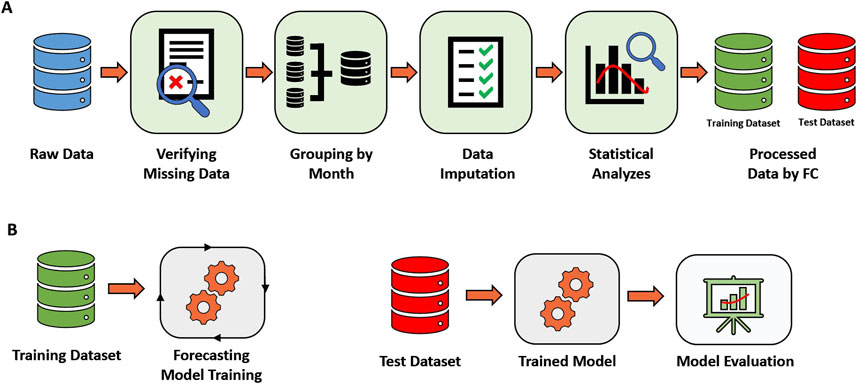
Figure 1. Proposed pipeline to process meteorological data and develop rainfall forecaster. (A) Preprocessing stage evolving missing data verification, data imputation, monthly data aggregation, and statistical analysis; (B) Stage of training and testing the model for monthly rainfall forecasting.

The first stage of the preprocessing pipeline consists of verifying whether there are missing data in the hourly data collected from the meteorological station. It is common for observed datasets to have gaps due to station defects or deterioration over time. Our investigation revealed that all the variables had missing values to some degree. Relative air humidity, wind direction, wind speed, atmospheric pressure, solar radiation (W/m²), and instant temperature (°C) presented 3.57% of missing data, whereas precipitation was collected with 4.76% of missing measures. Another important verification performed for the meteorological data was the assessment of missing data intermittency, that is, whether, within the same month, there were hours with both recorded and missing data. The analysis revealed no intermittency between available and missing data within the same month.

To address the issue of missing data, particularly in the context of sparse matrix processing, we first grouped the data by month for each meteorological variable, calculating cumulative monthly values for precipitation and average monthly values for the remaining variables. We subsequently applied data imputation by linear interpolation of values for each variable, where the missing values are estimated based on the preceding and succeeding observed values (Noor et al., 2014). Figure 2 shows the bar chart with the monthly precipitation level in Belém between 2016 and 2022 before the proposed data imputation strategy was applied (Figure 2A) and after the insertion of data (Figure 2B). The raw and imputed data for all the variables are provided in the Supplementary Material.

Figure 2

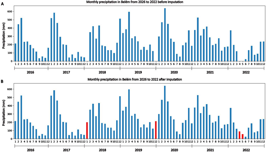
Figure 2. Monthly precipitation in Belém between 2016 and 2022 according to collected data. (A) Monthly precipitation before data imputation; (B) Monthly precipitation after data imputation.

The imputed covariates analyzed in this study, including relative humidity, wind direction, wind speed, atmospheric pressure, solar radiation, and instantaneous temperature between 2016 and 2022 are displayed in Figure 3. The solar radiation values between September 2019 and October 2021 are not zero but low, which can be associated with measurement problems in the meteorological station.

Figure 3

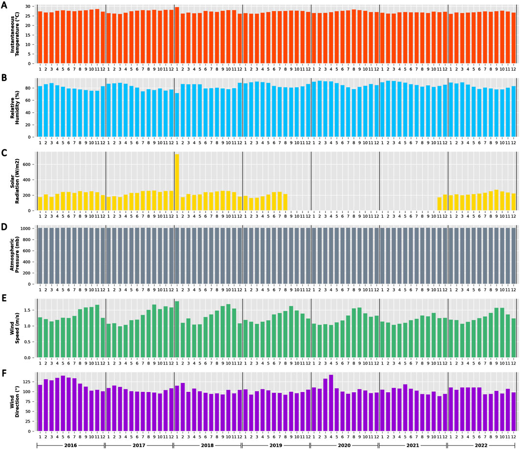
Figure 3. Imputed monthly meteorological variables between 2016 and 2022. (A) instant temperature (red bars); (B) relative humidity (blue bars); (C) solar radiation (yellow bars); (D) atmospheric pressure (gray bars); (E) wind speed (green bars); (F) wind direction (purple bars).

Autocorrelation, partial autocorrelation, and Spearman correlation analyses were conducted on the meteorological variables to assess the relation between the precipitation and its lagged values, and the relation between the meteorological covariates and monthly rainfall in Belém. These statistical tests are crucial for the last stage of the preprocessing pipeline, where training and test datasets are created according to FCs, which consist of groups of variables with varying levels of information. The training dataset consisted of meteorological data collected between 2016 and 2021, whereas the test dataset comprised meteorological data obtained for 2022.

2.2 Statistical and machine learning models

The statistical and ML models used in this work to perform monthly rainfall forecasting in Belém were autoregressive integrated moving average (ARIMA), seasonal autoregressive integrated moving average (SARIMA), seasonal autoregressive integrated moving average with exogenous inputs (SARIMAX), vector autoregressive moving average with exogenous regressors (VARMAX), long short-term memory (LSTM), and recurrent neural network (RNN) methods.

The ARIMA model is a statistical technique widely used for time series analysis, including applications in meteorology and financial market analysis (Falatouri et al., 2022). The ARIMA model can be expressed by ARIMA (p,d,q), where p, d, and q represent the order of the autoregressive model, the order of differences, and the order of the moving average, respectively. The mathematical formula of the ARIMA model is a combination of autoregressive, integrative, and moving average components (Alsharef et al., 2022; Shumway and Stoffer, 2017), as shown in Equation 1, where $y(t)\in \mathbb{R}$ and $ϵ\in \mathbb{R}$ are the observed value and the corresponding random disturbance of the series at time $t\in {\mathbb{Z}}^{+}$, respectively. The parameters $\varphi \in {\mathbb{R}}^p$ and $\theta \in {\mathbb{R}}^q$ are vectors of the model coefficients related to the autoregressive and moving average terms, respectively. The term ${\mathrm{\Delta }}^d$ represents the $d$-th derivative of an integrated component.

${\mathrm{\Delta }}^{d}y\left(t\right)={\displaystyle \sum _{j=1}^p}{\varphi }_{j}y\left(t-j\right)+{\displaystyle \sum _{k=1}^q}{\theta }_kϵ\left(t-k\right)+ϵ\left(t\right)(1)$

The SARIMA model is an extension of the ARIMA model that incorporates seasonal patterns in time series data (Korstanje, 2021). This technique can be represented by SARIMA (p,d,q) (P,D,Q)_S, where P, D, Q, and S are the orders of the seasonal autoregressive component, seasonal difference component, seasonal moving average, and seasonality period, respectively. The general SARIMA model can be expressed as shown in Equation 2. Similarly, the SARIMAX model aggregates the same properties as those from the previous models but incorporates exogenous input information (Alharbi and Csala, 2022; Arunraj et al., 2016), as shown in Equation 3.

${\mathrm{\Phi }}_P\left(B^S\right){\left(1-B^S\right)}^D{\varphi }_p\left(B\right){\left(1-B\right)}^{d}y\left(t\right)={\mathrm{\Theta }}_Q\left(B^S\right){\theta }_q\left(B\right)ϵ\left(t\right)(2)$

${\mathrm{\Phi }}_P\left(B^S\right){\left(1-B^S\right)}^D{\varphi }_p\left(B\right){\left(1-B\right)}^{d}y\left(t\right)={\mathrm{\Theta }}_Q\left(B^S\right){\theta }_q\left(B\right)ϵ\left(t\right)+\beta X\left(t\right)(3)$

The terms ${\mathrm{\Phi }}_P(B^S)\in {\mathbb{R}}^P$, ${\varphi }_p(B)\in {\mathbb{R}}^p$, ${\mathrm{\Theta }}_Q(B^S)\in {\mathbb{R}}^Q$, and ${\theta }_q(B)\in {\mathbb{R}}^q$ are the vectors associated with the regular autoregressive component, seasonal autoregressive component, regular moving average component, and seasonal moving average component, respectively. The elements ${(1-B)}^d$ and ${(1-B^S)}^D$ are operators of nonseasonal differentiation and seasonal differentiation, respectively, where $B$ represents the lag operator $(By(t)=y(t-1))$. The variable $X(t)\in {\mathbb{R}}^g$ represents the vector of exogenous inputs.

The VARMAX model is a multivariate statistical technique that enhances the vector autoregressive (VAR) technique and is designed to capture the dynamic relationships between multiple time series while considering the effects of integrating moving average components and exogenous variables (Gómez, 2019). Equation 4 presents the mathematical structure of the VARMAX model, where $Y(t)\in {\mathbb{R}}^g$ is the vector containing all the observable variables, $X(t)\in {\mathbb{R}}^g$ is the vector of exogenous variables, and $\xi (t)\in {\mathbb{R}}^g$ represents the vector of the corresponding random disturbances. The elements $\mathrm{\Phi }\in {\mathbb{R}}^{(g\text{x}g)}$, $\mathrm{\Theta }\in {\mathbb{R}}^{(g\text{x}g)}$, and $\mathrm{\Omega }\in {\mathbb{R}}^{(g\text{x}g)}$ are the matrices of autoregressive coefficients, moving average coefficients, and mapping coefficients of the exogenous regressors, respectively.

$Y\left(t\right)={\displaystyle \sum _{i=1}^p}\mathrm{\Phi }Y\left(t-i\right)+{\displaystyle \sum _{j=1}^q}\mathrm{\Theta }\xi \left(t-j\right)+\mathrm{\Omega }X\left(t\right)+\xi \left(t\right)(4)$

The best statistical model for rainfall forecasting in Belém was tuned for reproducibility using a grid search strategy associated with time series cross-validation (TSCV). The objective of this strategy was to select the model with the lowest value of the average root mean square error (avRMSE). The ranges of hyperparameters used to tune the statistical algorithms are detailed in Table 1.

Table 1

Table 1. Hyperparameters range used for Statistical Learning models.

RNN is a type of neural network in which connections between neurons allow signals to travel in loops, enabling the network to retain information across time steps. RNNs are connectionist models that represent sequential dynamics through cyclic patterns within a network structure, where the nodes are referred to as recurrent neurons (Lipton et al., 2015). Recurrent neurons rely on the current input and the output from the previous neuron in the network (Salem, 2022). This characteristic makes RNNs particularly well suited for time series prediction (Abbasimehr et al., 2020).

LSTM is an extension of RNNs. Its key feature is the inclusion of memory neurons in the hidden layers of the network architecture, which allows the LSTM to retain and utilize information from previous time steps, thereby improving its performance in time series analysis (Abbasimehr et al., 2020). The controlled flow of information among the memory neurons enables the LSTM model to capture and store various temporal dependencies with distinct characteristics (Lindemann et al., 2021).

Figure 4 illustrates the architectures of an RNN and an LSTM model with all relevant layers. The main difference between these models is the complexity of the mathematical operations for LSTM neurons. The RNN neurons only process the input and hidden state vectors using an activation function, as shown in Equation 5, where $W_h$, $U_h$, and $b_h$ are the weight matrix associated to input $X(t)$, the weight matrix associated with the hidden state $h(t-1)$, and the bias vector associated with the neuron, respectively. The LSTM neurons perform many operations to calculate the processed output via a forget gate, an input gate, candidate memory, and an output gate (Arras et al., 2019).

$ft=\sigma \left(W_{h}x\left(t\right)+U_{h}h\left(t-1\right)+b_h\right)(5)$

Figure 4

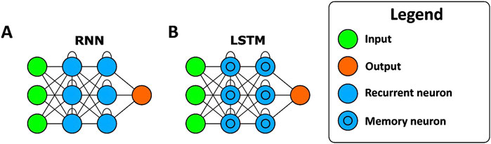
Figure 4. Artificial neural networks architectures. (A) Structure of recurrent neural network (RNN). (B) Structure of long short-term memory (LSTM).

For algorithms based on neural networks, the ranges of hyperparameters used for model tuning using the same grid search with TSCV as discussed above are shown in Table 2. To execute the algorithms, we used a machine with the following specifications: NVIDIA DGX H100 with 8 NVIDIA H100 Tensor Core GPUs, 640 GB of GPU RAM, 2 Intel Xeon Platinum 8480C CPUs, and 2 TB of system RAM.

Table 2

Table 2. Hyperparameters used for Machine Learning - Recurrent Neural Networks.

2.3 Model optimization and evaluation

The performance evaluation of the forecasting models proposed in this work is divided into two stages, as shown in Figure 1B. The first one consists of applying a grid search with TSCV to adjust the hyperparameters and select the model that achieves the lowest avRMSE value using the training data. TSCV is a cross-validation technique specifically designed for time series problems, which uses the training data to evaluate the model’s predictive performance. Initially, a training set (green bar) and a validation set (red bar) are defined based on their respective temporal window sizes, as illustrated in Figure 5. For each k-th fold of the TSCV, the training window is incrementally expanded, and the RMSE is computed on the corresponding validation data. The TSCV process concludes at the N-th fold, where the sum of the training and validation window sizes equals the total length of the training dataset. After all the RMSE values are calculated for all folds, the TSCV calculates the avRMSE. This approach allows the model to be trained on past data and tested on future data, thus accurately reflecting real-world scenarios (Bergmeir and Benítez, 2012). The second stage consists of evaluating the forecasting performance of the best-trained model using the RMSE for the test dataset.

Figure 5

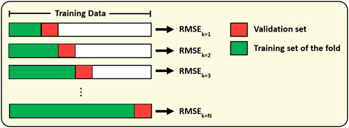
Figure 5. Schematic of time series cross-validation (TSCV) using expanding time window. Green bar represents the training set with expanding window and red bar represents the validation set in the k-th fold.

Equation 6 expresses the RMSE metric, where $y(t)$ and $\widehat{y}(t)$ are the real and the predicted result for the t-th measure, $\{t\in {\mathbb{Z}}^{+}|1\le t\le M\}$, respectively. Equation 7 presents the avRMSE formula, where k is the k-th fold and N is the total number of folds in TSCV, $\{k\in {\mathbb{Z}}^{+}|1\le k\le N\}$.

$\text{RMSE}=\sqrt{\frac{1}{M}{\displaystyle {\sum }_{t=1}^M}{\left(y\left(t\right)-\widehat{y}\left(t\right)\right)}^2}(6)$

$\text{avRMSE}=\frac{{\text{RMSE}}_{k=1}+{\text{RMSE}}_{k=2}+\cdots +{\text{RMSE}}_{k=N}}{N}(7)$

The second stage of the performance evaluation involves assessing the models according to the RMSE and absolute percentage error (APE) metrics for the months of the last year. Equation 8 shows the APE metric.

$\text{APE}=\left|\frac{y\left(t\right)-\widehat{y}\left(t\right)}{y\left(t\right)}\right|.100\%(8)$

3 Results

This section outlines the results obtained from the Spearman correlation and Granger causality test analyses conducted on the meteorological data during the preprocessing stage. Additionally, the data division process for feature composition analysis and the results of the performance analysis of the statistical and ML models for rainfall prediction in Belém are presented.

3.1 Statistical analysis of rainfall in Belém

Descriptive statistical analyses of the correlations between exogenous meteorological variables (inputs) and monthly precipitation (target) and analyses of autocorrelation functions are essential for extracting key insights into the climatic dynamics of Belém between 2016 and 2022, in addition to refining the dataset used for the development of predictive models. Figures 6A,B present the results obtained from applying autocorrelation and partial autocorrelation analysis between precipitation and lagged precipitation values.

Figure 6

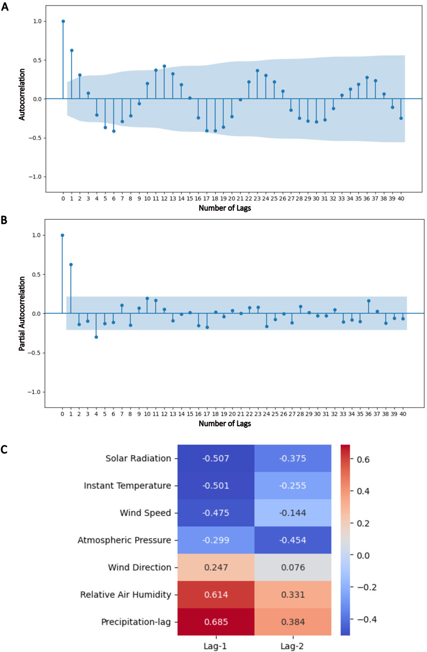
Figure 6. Statistical analysis for monthly precipitation in Belém. (A) Autocorrelation function for monthly precipitation in Belém by lag; (B) Partial autocorrelation functions for monthly precipitation in Belém by lag; (C) Spearman correlation of lagged meteorological variables with the monthly precipitation in Belém.

The autocorrelation analysis of monthly precipitation data in Belém reveals important insights into how the current accumulated precipitation is influenced by the values trends in previous months. The autocorrelation function shown in Figure 6A indicates that the current monthly precipitation value is strongly related to the value in the previous month (lag 1), reaching a correlation magnitude of 0.6245, whereas the values from subsequent months (lags 2, 3, 4, …) have little influence on the current rainfall value, with correlation magnitude of less than 0.4230. The p-value obtained for each autocorrelation by lag is less than 0.05, indicating that the correlation between the regressive values and the precipitation, mainly the lag 1, is statistically significant. The autocorrelation coefficients and their corresponding p-values are provided in Supplementary Table S1.

The contribution of lag 1 with precipitation prediction is also supported by the partial autocorrelation function analysis, which indicates that only precipitation data at lag 1, without the influence of other lags, exhibit a significant correlation with the current value, reaching a correlation of 0.632, exceeding the confidence interval region, as shown in Figure 6B.

The Spearman correlation results between exogenous meteorological variables at lags 1 and 2 and monthly precipitation indicate that relative air humidity, solar radiation, and instantaneous temperature at lag 1 are the environmental variables most strongly correlated with monthly rainfall in Belém, with absolute correlation values above 0.5, as shown in the heatmap in Figure 6C. However, this analysis also highlights that monthly precipitation at lag 1 itself has the strongest correlation with rainfall formation, which is corroborated by the p-value less than 0.05 for each correlation, indicating each correlation is statistically significative. On the other hand, none of the variables display a substantial correlation with monthly precipitation For lag 2, obtaining values less than 0.5 and p-value of 0.196 and 0.496 for wind speed and direction, respectively. The Spearman correlation coefficients and their corresponding p-values are available in Supplementary Table S2.

A comparison of the results obtained from both correlation analyses clearly reveals that the meteorological data at lag 1 exhibit stronger correlations with monthly precipitation, with a particular emphasis on previous precipitation trends and relative humidity. On the basis of these findings, we created datasets using the feature composition (FC) approach, in which the variables identified as most influential in the previous analyses for lag 1 (precipitation, relative air humidity, solar radiation, and instant temperature) were selected to establish a dedicated dataset for training and testing monthly precipitation prediction models. Table 3 summarizes how meteorological variables at lag 1 were grouped into FC classes, where FC-1 includes all variables, FC-2 consists only of the four selected variables, and FC-3 comprises only precipitation and relative humidity, as these two variables exhibited the highest correlations with current precipitation.

Table 3

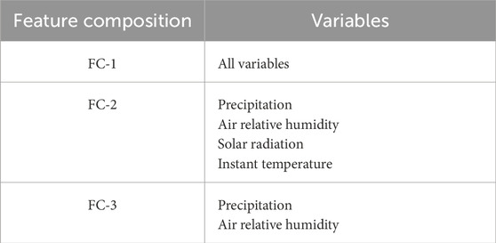
Table 3. Grouping of meteorological variables with lag 1 in feature composition.

3.2 Rainfall forecasting in Belém

Evaluating the impact of meteorological variables on the predictive modeling of monthly precipitation in Belém is essential for validating the statistical findings obtained from correlation analyses. Figure 7A presents a bar chart depicting the performance scores achieved by each statistical and ML model through TSCV. In contrast, Figure 7B illustrates the performance of these models in forecasting the total monthly precipitation for all months of 2022.

Figure 7

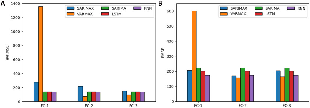
Figure 7. Performance evaluation of the statistical and machine learning models. (A) avRMSE values obtained by the models in the TSCV analysis by FC; (B) Performance of the models based on RMSE metric for monthly precipitation forecasting in 2022 by FC.

Figure 7A presents the performance evaluation of the predictive models based on the TSCV from 2016 to 2021. The results indicate that when all meteorological variables (FC-1) were utilized, the VARMAX model exhibited the worst performance, with an avRMSE of 1,354.89, whereas the other models achieved values below 276.86. However, by refining the models through the selection of meteorological variables with the highest correlations with monthly precipitation in Belém, the VARMAX model demonstrated a substantial performance improvement, with the avRMSE reduced to 74.75 and 93.90 for the variables included in FC-2 and FC-3, respectively. In contrast, neural network-based models (RNN and LSTM) did not display performance variations when the number of variables was reduced, which can be attributed to the training mechanism of these architectures, where the influence of less informative variables is naturally assigned a lower weight than those of more informative variables. Table 4 presents the optimized hyperparameters for the best prediction models based on their performance in TSCV. The performance of each model by hyperparameter in this analysis is displayed in Supplementary Tables S3–S7.

Table 4

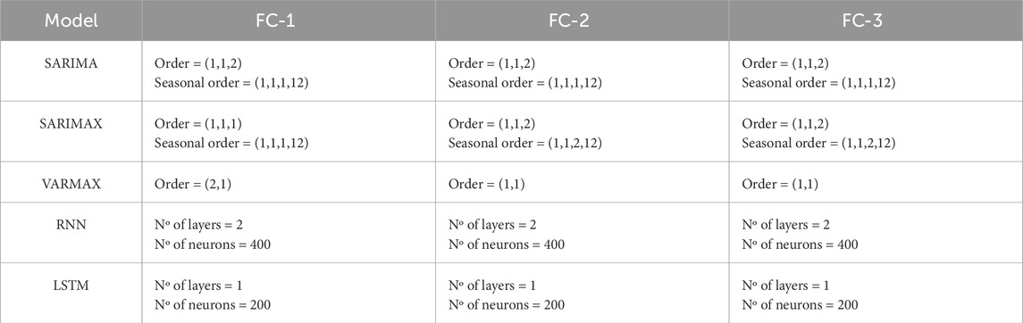
Table 4. Tuned hyperparameters from the best statistical and machine learning models.

The performance analysis of the best models based on FC analysis for monthly precipitation forecasting in Belém in 2022 is shown in Figure 7B. These results indicate a consistent performance trend compared with the outcomes obtained in the TSCV evaluation, particularly regarding the performance improvement observed for the SARIMAX and VARMAX models for FC-2 and FC-3. Among the analyzed models, the VARMAX model based on FC-2 achieved the lowest RMSE in this test, reaching a value of 156.70, whereas the other models yielded RMSE values above 170 when the same input variables were used.

Some important findings were also revealed in our predictive analyses. Figure 8 displays the observed precipitation values recorded at the meteorological station for each month in Belém in 2022 (blue bars). The other bars represent the monthly precipitation predicted by the best model with each technique, and the dashed line indicates the historical average for each month between 2016 and 2021. One key observation is that, for certain months in 2022, the observed precipitation values deviate significantly from the historical average, particularly between February and June. This temporal discrepancy in the temporal pattern between the training and test datasets is crucial for explaining why some models exhibited larger prediction errors for specific months, despite effectively capturing the overall trend of the historical average. Table 5 shows the values for observed, average and predicted monthly rainfall by model in 2022.

Figure 8

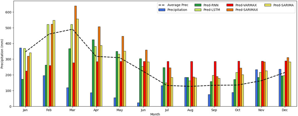
Figure 8. Comparison between observed precipitation (blue bars), historical average precipitation (dashed line), and the predicted monthly precipitation from the best-performing model.

Table 5

Table 5. Values of observed (last column), average (penultimate column), and predicted monthly rainfall by model in 2022 (first to fifth column).

Investigating the prediction error by month using APE metric, the models were able to predict rainfall effectively and yielded low APE values for the months between July and January of 2022 (dry season). For example, the VARMAX model based on FC-2, which achieved the best performance in the two tests, yielded values between 22.03% and 282.8% for these months, whereas the LSTM displayed values between 0.57% and 163.41% for the same period, as shown in Table 6. Evaluating the average APE for the 12 months, the LSTM model achieved the lowest value of 228.47%, as it best approximates the observed values, mainly for the dry season. On the other hand, for the rainy season, the models achieved higher error values, as can be seen for SARIMAX which obtained an APE of 1,503.71% for the month of June, while LSTM achieved the lowest value with 1,033.6% for the same month.

Table 6

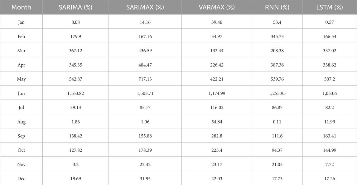
Table 6. Values of APE obtained by the models in each month of 2022.

4 Discussion

The rainfall dynamics in Belém are strongly modulated by environmental variables such as air temperature, wind speed and direction, solar radiation, and relative humidity, each contributing to precipitation variability at distinct levels. This is supported by the results of the Spearman correlation analysis conducted in this study, which reflect patterns typical of regions within the Amazon biome. Notably, as shown in Figure 6C, the most influential predictor for monthly rainfall was the precipitation observed in the preceding month, a finding further corroborated by autocorrelation plots.

In this timescale (seasonal scale), the phenomena that most affect tropical South America (including Belém) are El Niño-Southern Oscillation (ENSO) and Tropical Atlantic Gradient (Marengo et al., 2012; Reboita et al., 2021). The ENSO phenomena usually start in August of 1 year and ends in July of the following year (Tedeschi and Sampaio, 2022), while the most active phase of TAG is between March and May (MAM). During the period of this study (2016–2022), there were 2 EL Niños (2015/2016, 2018/2019) and 5 La Niñas (2016/2017, 2017/2018, 2020/2021, 2021/2022, and 2022/2023) (NOAA, 2025a). Although there was no positive TAG (AMM (Atlantic Meridional Mode) >1.0$°$C in MAM period), and the years 2018, 2019, 2021 and 2022 were negative TAG (AMM < −1.0$°$C) (NOAA, 2025b). The frequency of both phenomena affected the precipitation and its forecasting. It could also affect the future forecasting, mainly in neutral years (years without these phenomena).

The statistical analysis performed over the temporal window of data retrieved from the meteorological station reveals correlations between the long-term patterns of covariates and rainfall behavior over the 7-year period. Given the tropical climate of the Amazon region, which gives rise to two well-defined meteorological seasons (rainy and dry), the covariates exhibit distinctive seasonal trends. Among them, atmospheric pressure showed the least variability and thus the second-lowest correlation with rainfall (Spearman = −0.299), while wind direction displayed irregular patterns, resulting in the lowest correlation observed (Spearman = 0.247). In contrast, other variables, such as temperature and relative humidity, exhibited more consistent seasonal trends and correspondingly higher correlation values.

These climate-driven patterns directly influenced the performance of the rainfall forecasting models evaluated in this study. TSCV results demonstrated that the VARMAX model achieved the lowest avRMSE when using lag-1 values of monthly precipitation, relative humidity, solar radiation, and instantaneous temperature as inputs. This is particularly noteworthy, as this same configuration not only produced the lowest RMSE for forecasts in 2022 but also highlighted the importance of relative humidity (second-highest direct Spearman correlation) and solar radiation (highest inverse Spearman correlation) in enhancing predictive accuracy, even in the presence of data anomalies related to solar radiation measurements.

However, it is important to note that the precipitation levels observed in 2022 diverged from the historical average recorded during the training period (2016–2021), suggesting the presence of data drift. As shown in Figure 8, the SARIMA, SARIMAX, RNN, and LSTM models aligned more closely with the historical average than with the actual observed values (blue bars), indicating a systematic challenge in adapting to non-stationary climatic conditions. From a climatological perspective, this deviation may reflect broader impacts of global warming, which is progressively altering meteorological dynamics across the Amazon and introducing significant changes in precipitation patterns. These evolving conditions increase the magnitude of data drift, thereby making monthly rainfall prediction in this region increasingly complex. This hypothesis is supported by the high APE values observed during the rainy season across all trained models, as shown in Table 6.

5 Conclusion

Statistically investigating the associations between meteorological variables and precipitation levels is essential to understanding the influence that the dynamics of these environmental variables have on monthly rainfall formation in the city of Belém, which experiences high rainfall volumes between December and April, significantly impacting the city’s social dynamics.

Although there is a well-known difficulty in obtaining abundant and high-quality meteorological data from the Amazon region, mainly due to the scarcity of measurement stations and limited data accessibility, our analyses highlighted key aspects of the collected meteorological data, emphasizing that rainfall formation in Belém is intrinsically linked to certain environmental variables, primarily the rainfall volume in the previous month and relative humidity. On the other hand, other factors, such as solar radiation, instantaneous temperature, atmospheric pressure, wind speed, and wind direction, exhibited lower correlation levels with monthly rainfall in the capital of Pará.

From a predictive standpoint, although the amount of evaluated data is not substantial at the monthly scale—due to meteorological data availability limitations—the results highlight the strong potential of using statistical and ML models for learning tasks and precipitation forecasting. Our simulation results clearly demonstrate that the VARMAX model, which is based on the selection of the environmental variables with the highest correlations with the current precipitation volume (FC-2), achieves the best performance across all performance evaluation stages, yielding an RMSE value 8.97% lower than that of SARIMA, which is the second-best model in terms of monthly rainfall prediction for 2022. However, an in-depth analysis of the predictions revealed that the LSTM model achieved the best performance in terms of relative error, yielding the lowest average APE (2.28%) for forecasts throughout 2022. Unlike the VARMAX model, LSTM can capture the seasonal dynamics of precipitation data, which may have contributed to its higher accuracy in certain months. Therefore, these findings suggest that the proposed LSTM and VARMAX models trained with the meteorological variables with the highest correlations with the current precipitation volume are promising tools for operational monthly precipitation forecasting in Belém, potentially enhancing decision-making in the context of climate monitoring.

In future research, it would be beneficial to collect additional meteorological data from the city of Belém to perform additional spatiotemporal analyses at greater scales and assess the consistency of the resulting statistical correlations and predictions. Furthermore, expanding the dataset could enhance the training performance and robust of the predictive models by providing additional valuable information. Furthermore, the use of machine learning techniques such as deep learning, hybrid models, and transformer-based architectures like TimesNet, FEDformer, and TimeXer can also contribute to capturing the dynamic relationships between climatic variables and monthly precipitation in Belém, potentially improving forecasting performance metrics.

Data availability statement

The raw data supporting the conclusions of this article will be made available by the authors, without undue reservation.

Author contributions

EO: Conceptualization, Data curation, Formal Analysis, Investigation, Methodology, Software, Validation, Visualization, Writing – original draft, Writing – review and editing. EC: Supervision, Writing – original draft, Writing – review and editing. EJ: Data curation, Writing – review and editing. RR: Writing – review and editing. HA: Writing – review and editing. RA: Writing – review and editing. RT: Data curation, Funding acquisition, Project administration, Resources, Supervision, Validation, Writing – review and editing.

Funding

The author(s) declare that financial support was received for the research and/or publication of this article. This work was funded by Instituto Tecnológico Vale (ITV).

Conflict of interest

The authors declare that the research was conducted in the absence of any commercial or financial relationships that could be construed as potential conflicts of interest.

Generative AI statement

The authors declare that no Generative AI was used in the creation of this manuscript.

Publisher’s note

All claims expressed in this article are solely those of the authors and do not necessarily represent those of their affiliated organizations, or those of the publisher, the editors and the reviewers. Any product that may be evaluated in this article, or claim that may be made by its manufacturer, is not guaranteed or endorsed by the publisher.

Supplementary material

The Supplementary Material for this article can be found online at: https://www.frontiersin.org/articles/10.3389/feart.2025.1589753/full#supplementary-material

References

Abbasimehr, H., Shabani, M., and Yousefi, M. (2020). An optimized model using lstm network for demand forecasting. Comput. Industrial Eng. 143, 106435. doi:10.1016/j.cie.2020.106435

CrossRef Full Text | Google Scholar

Alharbi, F. R., and Csala, D. (2022). A seasonal autoregressive integrated moving average with exogenous factors (SARIMAX) forecasting model-based time series approach. Inventions 7, 94. doi:10.3390/inventions7040094

CrossRef Full Text | Google Scholar

Alsharef, A., Aggarwal, K., Sonia, S., Kumar, M., and Mishra, A. (2022). Review of ML and AutoML solutions to forecast time-series data. Archives Comput. Methods Eng. 29, 5297–5311. doi:10.1007/s11831-022-09765-0

PubMed Abstract | CrossRef Full Text | Google Scholar

Alves, L. M., Chadwick, R., Moise, A., Brown, J., and Marengo, J. A. (2021). Assessment of rainfall variability and future change in Brazil across multiple timescales. Int. J. Climatol. 41, E1875–E1888. doi:10.1002/joc.6818

CrossRef Full Text | Google Scholar

Arras, L., Arjona-Medina, J., Widrich, M., Montavon, G., Gillhofer, M., Müller, K.-R., et al. (2019). Explaining and interpreting LSTMs. Cham: Springer International Publishing, 211–238. doi:10.1007/978-3-030-28954-6_11

CrossRef Full Text | Google Scholar

Arunraj, N. S., Ahrens, D., and Fernandes, M. (2016). Application of sarimax model to forecast daily sales in food retail industry. Int. J. Operations Res. Inf. Syst. (IJORIS) 7, 1–21. doi:10.4018/ijoris.2016040101

CrossRef Full Text | Google Scholar

Bergmeir, C., and Benítez, J. M. (2012). On the use of cross-validation for time series predictor evaluation. Inf. Sci. 191, 192–213. doi:10.1016/j.ins.2011.12.028

CrossRef Full Text | Google Scholar

Costa, G. R. d. S., Blanco, C. J. C., da Silva Cruz, J., and de Mendonça, L. M. (2024). Estimating the daily flooding probability by the compound effect of rainfall and tides in an Amazonian metropolis. Urban Clim. 57, 102121. doi:10.1016/j.uclim.2024.102121

CrossRef Full Text | Google Scholar

Damor, P. A., Mod, A. A., Ram, B., and Parmar, H. V. (2024). Time series analysis and development of simulation model for monthly rainfall using ARIMA model. Int. J. Agric. Sci. 20, 226–235. doi:10.15740/HAS/IJAS/20.1/226-235

CrossRef Full Text | Google Scholar

Falatouri, T., Darbanian, F., Brandtner, P., and Udokwu, C. (2022). Predictive analytics for demand forecasting–a comparison of sarima and lstm in retail scm. Procedia Comput. Sci. 200, 993–1003. doi:10.1016/j.procs.2022.01.298

CrossRef Full Text | Google Scholar

Ferreira, G. S. E., and Medeiros, D. (2022). Uma avaliação de algoritmos de regressão para predição de volume de chuva. in An. do XL Simpósio Bras. Telecomunicações Process. Sinais Soc. Bras. Telecomunicações, 2–3. doi:10.14209/sbrt.2022.1570817471

CrossRef Full Text | Google Scholar

Gómez, V. (2019). “VARMAX and transfer function models,” in Linear time series with MATLAB and OCTAVE, 121–172. doi:10.1007/978-3-030-20790-8_3

CrossRef Full Text | Google Scholar

Guideli, L. C., dos Reis Cuenca, A. L., Silva, M. A., and de Brum Passini, L. (2021). Road crashes and field rainfall data: mathematical modeling for the brazilian mountainous highway br-376/pr. Transportes 29, 2498. doi:10.14295/transportes.v29i4.2498

CrossRef Full Text | Google Scholar

Han, W., Zhang, X., Wang, Y., Wang, L., Huang, X., Li, J., et al. (2023). A survey of machine learning and deep learning in remote sensing of geological environment: Challenges, advances, and opportunities. ISPRS J. Photogrammetry Remote Sens. 202, 87–113. doi:10.1016/j.isprsjprs.2023.05.032

CrossRef Full Text | Google Scholar

Hawthorne, S., Wang, Q. J., Schepen, A., and Robertson, D. (2013). Effective use of general circulation model outputs for forecasting monthly rainfalls to long lead times. Water Resour. Res. 49, 5427–5436. doi:10.1002/wrcr.20453

CrossRef Full Text | Google Scholar

Hussain, A., Aslam, A., Tripura, S., Dhanawat, V., and Shinde, V. (2024). Weather forecasting using machine learning techniques: rainfall and temperature analysis. J. Adv. Info. Tech. 15, 1329–1338. doi:10.12720/jait.15.12.1329-1338

CrossRef Full Text | Google Scholar

Ioannou, K., Karampatzakis, D., Amanatidis, P., Aggelopoulos, V., and Karmiris, I. (2021). Low-cost automatic weather stations in the internet of things. Information 12, 146. doi:10.3390/info12040146

CrossRef Full Text | Google Scholar

Korstanje, J. (2021). Advanced forecasting with Python. Berkeley, CA: Apress. doi:10.1007/978-1-4842-7150-6

CrossRef Full Text | Google Scholar

Lindemann, B., Müller, T., Vietz, H., Jazdi, N., and Weyrich, M. (2021). A survey on long short-term memory networks for time series prediction. Procedia CIRP 99, 650–655. doi:10.1016/j.procir.2021.03.088

CrossRef Full Text | Google Scholar

Lipton, Z. C., Berkowitz, J., and Elkan, C. (2015). A critical review of recurrent neural networks for sequence learning. ArXiv abs/1506, 00019.

Google Scholar

Lorenz, E. N. (2005). Designing chaotic models. J. Atmos. Sci. 62, 1574–1587. doi:10.1175/jas3430.1JAS3430.1

CrossRef Full Text | Google Scholar

Luiz-Silva, W., Oscar-Júnior, A. C., Cavalcanti, I. F. A., and Treistman, F. (2021). An overview of precipitation climatology in Brazil: space-time variability of frequency and intensity associated with atmospheric systems. Hydrological Sci. J. 66, 289–308. doi:10.1080/02626667.2020.1863969

CrossRef Full Text | Google Scholar

Luo, Q. (2024). Decoding Pakistan’s rainfall: optimizing predictions from ARIMA to SARIMA with seasonal adjustments. Theor. Nat. Sci. 42, 73–83. doi:10.54254/2753-8818/42/2024CH0215

CrossRef Full Text | Google Scholar

Ma, Q., Li, Y., Feng, H., Yu, Q., Zou, Y., Liu, F., et al. (2021). Performance evaluation and correction of precipitation data using the 20-year imerg and tmpa precipitation products in diverse subregions of China. Atmos. Res. 249, 105304. doi:10.1016/j.atmosres.2020.105304

CrossRef Full Text | Google Scholar

Marengo, J., Liebmann, B., Grimm, A., Misra, V., Silva Dias, P., Cavalcanti, I., et al. (2012). Recent developments on the south american monsoon system. Int. J. Climatol. 32, 1–21. doi:10.1002/joc.2254

CrossRef Full Text | Google Scholar

Mendoza, R. R. (2018). Analysis of precipitation in Belém-PA city (period 1967-2016). Int. J. Hydrology 2. doi:10.15406/ijh.2018.02.00088

CrossRef Full Text | Google Scholar

Monteiro, L. A. F., do Nascimento, F. I. C., de Oliveira-Júnior, J. F., Nunes, D. D., Mendes, D., de Gois, G., et al. (2024). Rainfall projections for the Brazilian legal Amazon: an artificial neural networks first approach. Climate 12, 187. doi:10.3390/cli12110187

CrossRef Full Text | Google Scholar

NOAA (2025a). Historial el nino/la nina episodes (1950-present). Available online at: https://origin.cpc.ncep.noaa.gov/products/analysis_monitoring/ensostuff/ONI_v5.php (Accessed April 24, 2025).

Google Scholar

NOAA (2025b). Atlantic meridional mode dataset. Available online at: https://psl.noaa.gov/data/timeseries/monthly/AMM/ammsst.data (Accessed April 24, 2025).

Google Scholar

Noor, N. M., Al Bakri Abdullah, M. M., Yahaya, A. S., and Ramli, N. A. (2014). Comparison of linear interpolation method and mean method to replace the missing values in environmental data set. Mater. Sci. Forum 803, 278–281. doi:10.4028/www.scientific.net/MSF.803.278

CrossRef Full Text | Google Scholar

Novák, Z., Juhász, L., and Varga, S. Z. (2020). Significance of local meteorological stations in research planning. Acta Agrar. Debreceniensis, 87–91. doi:10.34101/actaagrar/2/37402/3740

CrossRef Full Text | Google Scholar

Pinheiro Gomes, E., Progênio, M. F., and da Silva Holanda, P. (2024). Modeling with artificial neural networks to estimate daily precipitation in the Brazilian legal Amazon. Clim. Dyn., 6219–6233. doi:10.1007/s00382-024-07200-7

CrossRef Full Text | Google Scholar

Pirone, D., Cimorelli, L., Del Giudice, G., and Pianese, D. (2023). Short-term rainfall forecasting using cumulative precipitation fields from station data: a probabilistic machine learning approach. J. Hydrology 617, 128949. doi:10.1016/j.jhydrol.2022.128949

CrossRef Full Text | Google Scholar

Reboita, M., Ambrizzi, T., Crespo, N., Dutra, L., Ferreira, G., Rehbein, A., et al. (2021). Impacts of teleconnection patterns on south America climate. Ann. N. Y. Acad. Sci. 1504, 116–153. doi:10.1111/nyas.145921111/nyas.14592

PubMed Abstract | CrossRef Full Text | Google Scholar

Reigosa, C. J., Serrano, M., Justavino, M., and Villarreal, V. (2024). “Integrated climate observation and analysis system for scientific research,” in 2024 IEEE VII Congreso Internacional en Inteligencia Ambiental, Ingeniería de Software y Salud Electrónica y Móvil (AmITIC) (IEEE), 1–5. doi:10.1109/AmITIC62658.2024.10747588

CrossRef Full Text | Google Scholar

Salem, F. M. (2022). Recurrent neural networks: from simple to gated architectures. Springer International Publishing.

CrossRef Full Text | Google Scholar

Santos, D. M. N., Rocha, Y. A. S., Freitas, D., Beltrão, P., Santos Junior, P., Marques, G., et al. (2021). Time-series forecasting models. Int. J. Innovation Educ. Res. 9, 24–47. doi:10.31686/ijier.vol9.iss8.3239ijier.vol9.iss8.3239

CrossRef Full Text | Google Scholar

Shumway, R. H., and Stoffer, D. S. (2017). Time series analysis and its applications: with R examples. Springer International Publishing, 289–384. doi:10.1007/978-3-319-52452-8-6

CrossRef Full Text | Google Scholar

Tedeschi, R. G., and Sampaio, G. (2022). Influences of different intensities of el niño–southern oscillation on south American precipitation. Int. J. Climatol. 42, 7987–8007. doi:10.1002/joc.7688

CrossRef Full Text | Google Scholar